Characterization of F-region neutral wind response times and its controlling factors during substorms

Ion-neutral coupling is responsible for dissipating energy deposited into the high-latitude ionosphere during geomagnetically active periods. The neutral wind response time, or the ion-neutral coupling efficiency, is not well characterized, with a wide range of reported response times. Additionally, how this coupling efficiency varies with geomagnetic activity level is not well understood, with few studies addressing the impact of geomagnetic activity level on neutral wind response time. In this study, a statistical analysis of the neutral wind response time during substorm periods is performed. We use data from Scanning Doppler Imagers (SDIs) and the Poker Flat Incoherent Scatter Radar (PFISR) to calculate the neutral wind response time using the new weighted windowed time-lagged correlation method. Substorm events were found using SuperMAG substorm lists and All Sky Imagers (ASIs). This statistical analysis resulted in 23 substorm events, with an average response time of $\sim$16 min. To determine the controlling factors of this response time, geomagnetic and ionospheric parameters, such as IMF strength and orientation, SYM/H index, AE index, and electron density, are investigated for the statistical substorm set. A superposed epoch analysis of the parameters is performed to determine average geospace conditions required for fast neutral wind responses. It was found that quiet-time conditions in AE and SYM-H indices, a southward turning of IMF around 1.5 h before substorm onset time, and large electron densities lead to faster neutral wind response times. Based on the geomagnetic indices results, it was suggested that thermospheric pre-conditioning may play a role in neutral wind response times.

1 Introduction

High-latitude ionosphere-thermosphere coupling is a crucial dynamic for dissipating energy deposited into Earth’s upper atmosphere during geomagnetic storms and substorms. Ionosphere-thermosphere coupling in the form of ion-neutral collisions create an ion-drag force, which sets the F-region neutral atmosphere in motion. The resulting thermospheric winds redistribute mass and energy deposited into Earth’s upper atmosphere. However, because the thermosphere is more massive than the ionosphere, and is also subjected to pressure-gradient, advection, and other forces, the neutral wind response will often be delayed from changes in ionospheric flow. This time delay, or neutral wind response time, is a key indicator of the ion-neutral coupling efficiency, and it is not well understood. Additionally, the controlling factors of this coupling efficiency, such as geomagnetic activity strength or ionospheric parameters, are not well characterized.

It is important to know whether the coupling efficiency strengthens as geomagnetic activity strength increases since ion-neutral coupling is responsible for dissipating the high-latitude energy deposited during substorms. This parameter would affect how long the ionosphere remains highly-energized, putting LEO satellites at risk of increased satellite drag and de-orbit. It is generally understood that an increase in geomagnetic activity level will increase ion-neutral coupling through an enhanced electron density, therefore decreasing the neutral wind response time. Faster neutral wind responses for higher levels of geomagnetic activity have also been observed. For example, Kosch et al. (2001) used the Kp index to indicate a geomagnetically active and quiet period of time, and found that the e-folding time was 1.8 and 3.3 h for an active and quiet period, respectively. Ponthieu et al. (1988) studied the response times during a solar maximum event and solar minimum event, and found that the e-folding time during solar minimum was an order of magnitude larger than at solar maximum. A statistical study of 902 nights spanning across solar maximum and solar minimum years found that geomagnetic polar cap wind speeds were around 200 m/s in solar minimum and 800 m/s in solar maximum, with a strong dependence on Kp index (Killeen et al., 1995). These studies focused more on large-scale differences of the neutral wind response time, studying the effects of solar maximum vs. solar minimum or geomagnetic storm vs. geomagnetic quiet time.

While geomagnetic storms cause a large-scale magnetospheric disturbance lasting a few days, substorms are explosive releases of energy lasting only about 1–3 h (Tanskanen, 2009). It has been shown that the energy deposited into the high-latitude ionosphere can range from 30% up to 100% of the magnetic energy stored in the magnetotail during substorms (Tanskanen et al., 2002; Akasofu, 2013; Spencer et al., 2019). This explosive release causes rapid changes in the high-latitude ionospheric convection. Reconfiguration of the ionospheric convection pattern occurs on the time scale of minutes (Wing et al., 2002; Yu and Ridley, 2009). In addition to rapid reconfiguration, plasma flow has also been shown to increase on the order of hundreds to thousands of meters per second over intervals of 10–20 min (Sánchez et al., 1996). Neutral winds are driven by these rapid flows due to increased ion-neutral collisions from substorm associated particle precipitation. However, the neutral wind response time during these intense substorm injections are not well characterized. Previous studies typically use observational methods to determine the neutral wind response time during substorms, which leads to a wide range of reported response times, from immediate responses to a time scale of tens of minutes (Cai et al., 2019; Billett et al., 2020; Zou et al., 2021).

Substorms also cause a significant enhancement in energetic particle precipitation, with the power of diffuse, monoenergetic, and wave electron aurora having been shown to increase by 310%, 71%, and 170%, respectively, during a substorm cycle (Wing et al., 2013). While electron density enhancements due to substorms typically peak in the E-region altitudes (Kaeppler et al., 2020; Grandin et al., 2024; Oyama et al., 2014), the thermosphere in this region is much denser and ion-neutral collisions here often impede ionospheric ExB drift (Sangalli et al., 2009). Therefore, neutral wind responses to plasma convection are typically much slower in the E-region, on the order of hours (Richmond et al., 2003; Billett et al., 2020). The F-region, however, still sees significant electron density enhancements during substorms. During substorm recovery, quasiperiodic brightenings of the aurora, known as pulsating aurora (Jones et al., 2011), have been shown to be associated with soft electron precipitation in the F-region (Oyama et al., 2014; Fukizawa et al., 2021). A case study done by Liu et al. (2008) used the NORSTAR multispectral imager (MSI) and found equatorward moving streamers in the 630.0 nm emission line (F-region) prior to substorm onset. Kepko et al. (2009) observed an equatorward moving diffuse auroral patch in the 630.0 nm emission line just before substorm onset. Gillies et al. (2017) used a REGO ASI and the Resolute Bay Incoherent Scatter Radar-Canadian (RISR-C) to study 630.0 nm auroral emissions and found that at the 220–240 km altitude range, electron density increased within red discrete arcs and in the region of diffuse aurora. This evidence shows that the F-region thermosphere would be subjected to a significant ion-drag force during substorms due to the enhanced precipitation, however it is still unclear how efficient this forcing is.

Similarly, few studies have been done regarding the relative strength of geomagnetic activity on neutral wind response, e.g., the response during a 300 nT substorm vs. the response during a 600 nT substorm. One such study was performed by Omaya et al. (2023), where hourly mean winds from 9 years of FPI data were binned by a SuperMAG (SME) index and found that zonal dusk winds had larger westward flows for increased SME. Another study by Zou et al. (2021) constructed a statistical wind morphology as a function of magnetic latitude, local time and ${\text{AE}}^{*}$ index and also found that wind speeds increased as ${\text{AE}}^{*}$ increased, with ${\text{AE}}^{*}$ being the maximum AE value in the past 2 hours of individual measurements. While these studies show that neutral winds have a dependence on the strength of geomagnetic activity level, there is still limited information on how the neutral wind response time, and the ion-neutral coupling efficiency, varies with geomagnetic activity level.

In this study, we perform a statistical analysis of the neutral wind response time and its controlling factors during substorm periods. Section 2 describes the instrumentation, event selection criteria, and methodology. Section 3.1 provides the results of the statistical survey, and Sections 3.2 and 3.3 details two case studies from the event list. Sections 3.4 and 3.5 presents a superposed epoch analysis of the geomagnetic conditions and electron density of the events, respectively, and Section 3.6 discusses other possible controlling factors of the neutral wind response time. The work is summarized in Section 4.

2 Materials and methods

2.1 Scanning Doppler Imagers

The 630.0 nm emissions from the Poker Flat (PKR, 65.1$°$N, −147.5$°$E) and Toolik Lake (TLK, 68.6$°$N, −149.6$°$E) Scanning Doppler Imager (SDI) are used to observe thermospheric parameters (Conde and Smith, 1995; 1997; 1998; Conde and Nicolls, 2010). The 630.0 nm emission spectra originate from atomic oxygen around 230 km, placing our observations in the F-region thermosphere. SDIs are Fabry-Perot interferometers that observe emission spectra in 115 subregions of the field-of-view (FOV). Line-of-sight (LOS) velocities for each subregion are inferred from the Doppler shifts, with the rest wavelength derived from the average spectra of the entire FOV. Horizontal wind vectors are derived from the LOS velocities using a monostatic fitting method, which assumes that vertical winds are constant across the FOV and the zonal gradient of meridional winds is negligible. The calculation method is derived thoroughly in Conde and Smith (1998). The resulting horizontal wind vectors have a spatial resolution of 0.5$°$ at the zenith and 1$°$ near the FOV edge. The FOV of the SDIs are around 10$°$ in diameter. The wind vectors have a temporal resolution of 1–5 min. Errors in the monostatically fit wind vectors are estimated to be <15–20 m/s (Anderson et al., 2012a; b; Dhadly et al., 2015). Thermospheric winds have been shown to deviate from quiet time averages by nearly 500 m/s during geomagnetically active periods (Omaya et al., 2023), and therefore our storm and substorm focused events will have wind variations much larger than the wind errors.

2.2 Poker Flat Incoherent Scatter Radar

The Poker Flat Incoherent Scatter Radar (PFISR) (65.1$°$N, −147.5$°$E geographic) is an Advanced Modular Incoherent Scatter Radar (AMISR) and is used to measure ionospheric parameters. PFISR is a phased array radar, which allows for multi-directional scanning and faster scanning than dish antenna radars, leading to higher spatial and temporal resolutions. Long pulse mode is employed, which targets the F-region ionosphere. Radio waves are incoherently scattered from the free electrons in the ionosphere, and the return power yields the electron density. The Doppler shift of the return spectra provides the LOS ion drift velocity. Similar to the SDIs, the LOS velocities are inverted into horizontal drift vectors by assuming that the velocity vectors are homogeneous in the east-west direction across the radar FOV. Errors arise from the nonlinear least squares fitting procedure, and are provided along with the horizontal velocity vectors. A more detailed methodology is provided in Heinselman and Nicolls (2008). Spatial and temporal resolution, as well as spatial FOV, varies based on the beam orientations of various experiment modes. The FOV ranges from 2–4$°$ MLAT with a spatial resolution of 0.25$°$ - 0.5$°$, and temporal resolution of 1–5 min.

This study uses an updated version of the Heinselman and Nicolls (2008) algorithm that makes strict use of Modified Apex coordinates (Richmond, 1995; Laundal and Richmond, 2017) to solve for the covariant components of the velocity more rigorously, then transforms back into standard geodetic vectors. Furthermore it applies filtering based on quality flags in the LoS data and makes use of robust error propagation to nominally improve the estimates of 3D velocity (Lamarche, 2024).

PFISR is also used to obtain electron density profiles for the upper atmosphere. The area of the return spectra provides the electron density for each beam of the radar. This area is corrected for the damping of the spectra due to the ratio of the electron to ion temperature. Each beam configuration has a beam that is parallel to the magnetic field line, at an elevation angle of 77.5$°$. We use the electron density profile along this beam so that we are observing electron density enhancements due to particle precipitation.

2.3 Time history of events and Macroscale Interactions during substorms ground-based observatories

The Time History of Events and Macroscale Interactions during Substorms all-sky imagers (THEMIS ASIs (Mende et al., 2008)) are white light CCD cameras that are used to capture auroral patterns. Images are recorded at a cadence of 3 s and projected onto an altitude of 110 km. The Fort Yukon (FYKN; geographic ${66.6}^o$N, ${-145.2}^o$N) and Gakona stations (GAKO, ${62.4}^o$N, ${-145.2}^o$E) are mainly used, which have large common FOVs with the SDIs. The ASIs have a circular FOV with around a 9$°$ diameter, and a spatial resolution of around 1 km at the zenith and a temporal resolution of 3 s.

In addition to the ASIs, each THEMIS ground-based observatory (GBO) contains a fluxgate magnetometer (GMAG) (Russell et al., 2009). The magnetometers provide 3-component magnetic field measurements, North-South, East-West, and Vertical, with a 2 Hz cadence. The measurements correspond to a 100 km radius region about 100 km above the GBO.

2.4 OMNI data

High-resolution (1- and 5-min) solar wind magnetic field and plasma data sets are provided by NASA/GSFC’s Space Physics Data Facility’s OMNIWeb service. The OMNI data set is attained by time shifting magnetic field and plasma data from the Wind, ACE, IMP eight and Geotail satellites from the satellite location to Earth’s bow shock, accounting for the propagation time of the solar wind. The data used from the OMNI data set includes the interplanetary magnetic field (IMF) measurements as well as the AE and SYM/H indices, which are computed at the WDC for Geomagnetism at the University of Kyoto. It is important to note that the IMF conditions are the conditions at the bow shock, and the solar wind will take an additional $\sim$7–10 min to reach the magnetopause (Cousins and Shepherd, 2010). However, in this study we are more concerned with the trend of IMF conditions between events, so no additional shift is made for our analysis.

2.5 Event selection criteria and methodology

A search was performed from 2012–2015 for substorm events using both the Newell and Gjerloev (2011) and Forsyth et al. (2015) SuperMAG substorm lists. Both lists utilize the SuperMAG AL (SML) index in order to identify substorms. While there is some variation in methodology between the two lists, both are used in order to increase the possible number of substorm events. Because these lists use the SML index to identify substorms, they may include both magnetospheric and auroral substorms. Magnetospheric substorms are classified by an energy dissipation in the nightside auroral oval and auroral substorms are defined by the auroral signature, which includes a brightening of the equatorward auroral arc followed by poleward expansion (Rostoker et al., 1980; Akasofu, 1964; Nishimura and Lyons, 2021). Auroral substorms will have signatures of a magnetospheric substorm, but magnetospheric substorms will not always have the associated auroral substorm signatures. Nevertheless, we are looking for events with enhanced geomagnetic activity and sudden plasma enhancements that may be imposed upon the neutral wind, which can occur for both magnetospheric and auroral substorms, making the SuperMAG substorm lists suitable for this study.

One requirement was that the substorm events are not coincident with large geomagnetic storms (SYM/H <−50 nT), since storms are associated with large, global-scale variations of the plasma and neutral populations and in this study, we are more interested in the local effects of substorm forcing. For the substorm events, simultaneous operations of PFISR and SDI were required, and it was preferred to have ASI operations for each event. Additional requirements were clear sky conditions (no cloud coverage) in ASI and SDI data, and relatively low error (<20$\%$) in the derived PFISR velocity vectors provided by AMISR. Because the instruments provide data around 62$°$ - 72$°$ magnetic latitude and the SDIs and ASIs only operate in the nighttime, the substorm onsets are limited to nightside auroral oval, between 07:00 UT and 14:00 UT and 20–03 MLT, where 11:00 UT corresponds to magnetic midnight in the Alaskan region. It was also required that substorm onsets occurred near the observation sites in order to ensure a response can be observed in the ionosphere and thermosphere. This means substorms whose growth phase or poleward expansion phase crosses over the data FOV. It is also preferred to have substorm onset MLT within 2 h of the SDI MLT, however, events that fell out of this location range were still included if a neutral wind response was observed. Events where no response is observed in either the neutral wind vectors or plasma flow vectors were omitted, which can occur if substorm onset is near magnetic midnight, at which the neutral winds can be subject to the strong cross-polar jet (Conde et al., 2001; Smith et al., 1998; Meriwether Jr. et al., 1988). We defined responses of the plasma flow to be a change of around 500 m/s in 20 min and responses of the wind to be around 50 m/s in 30 min. This search resulted in 23 events over the 4 year period. Though there were many more substorms during this period, it is difficult to fulfill all requirements for each substorm event due to frequent cloud coverage in the Alaska region, resulting in a relatively low event number. However, trends in the neutral wind response time were still observed with our event list.

SDI data is obtained in the form of skymap, aligned geomagnetically, with zonal and meridional wind vectors at each viewing location of the SDI from the Monthly Data Archive maintained by UAF. To make keograms, or latitude vs. time plots, of the zonal and meridional winds, data is binned by 1$°$ latitude and a center slice is taken 2.5$°$ east and west of the central magnetic longitude. The data is averaged over each latitude bin for smoothing. PFISR eastward/northward velocity vectors are obtained from MadrigalWeb in the form of keograms, in geomagnetic coordinates. Both the PFISR and SDI data are interpolated to a 5 min interval time-series, which is the average sampling time for both data-sets. This is done because SDI and PFISR have different recorded data times, and need to be interpolated to a common time interval in order to run the analysis. The PFISR data is then smoothed in time by taking a sliding 10 min (two data point) average. This is because the plasma can be highly variable due to the rapidly changing magnetospheric coupling (Murr and Hughes, 2001), and only the meso-to large-scale responses to substorms are relevant for this study. Finally, auroral keograms are obtained from the aurora-asi-lib python package developed by Shumko et al. (2022).

For each event, a time-series of the zonal plasma and neutral wind velocity was selected at a single latitude, within 1$°$ of each other. The main focus of this study is the zonal direction because in the pre-midnight sector, where most our substorm events occur, ion convection is primarily aligned in the east-west direction along the eastward electrojet and therefore do not see much response in the meridional direction compared to the zonal direction (Davidson et al., 2024; Zou et al., 2018). Neutral wind response times were then calculated by performing a weighted windowed time-lagged correlation (WWTLC) analysis, as described by Davidson et al. (2024). This method provides a time-dependent, observation based response time, with a lag time every 15 min. The e-folding time was additionally calculated, which is a theory based calculation of the neutral wind response time which assumes ion-drag is the only driving force. The Equation 1, first derived by Baron and Wand (1983), is given as

$\tau =\frac{\mathit{V}-\mathit{U}}{\partial \mathit{U}/\partial t}(1)$

where V is the horizontal plasma vector and U is the horizontal wind vector. The time-series data has a 5-min temporal resolution, and therefore the e-folding time calculation gives a neutral wind response time every 5 min.

3 Results and discussion

3.1 Statistical summary

A summary of the 23 events can be found in Table 1. From left to right, this table includes the date, SuperMAG substorm onset time, WWTLC time range, WWTLC time of the substorm window, e-folding time range, and e-folding time median of the substorm window. The substorm window is defined as the 2 h window with the substorm onset at its midpoint. This study focused on this substorm onset window in order to study the neutral wind’s immediate response to substorm forcing. Substorm onset WWTLC response times ranged from 0–70 min, with an average response time of $\sim$16 min. This response time is in line with the more recent observed neutral wind response times on the order of tens of minutes (Aruliah and Griffin, 2001; Anderson et al., 2011; Conde et al., 2018; Zou et al., 2018). The substorm window e-folding times ranged from 69–163 min, with an average of 109 min. This is significantly longer than the WWTLC response times. However, as discussed in Davidson et al. (2024), the e-folding time may not be fully representative of the neutral wind response time. Therefore, only the WWTLC response times are used to study the controlling factors of the neutral wind response time. To investigate the controlling factors of the neutral wind response time, short and long response time events are first defined. Based on the average response time of $\sim$16 min, short response time events are classified as those with response times ≤15 min and long response time events are defined as those with response times ≥20 min. This grouping resulted in 15 short response time events and eight long response time events. Then, the IMF conditions and ionospheric parameters were studied for short and long response events, respectively, to determine any controlling factors of the neutral wind response time.

Table 1

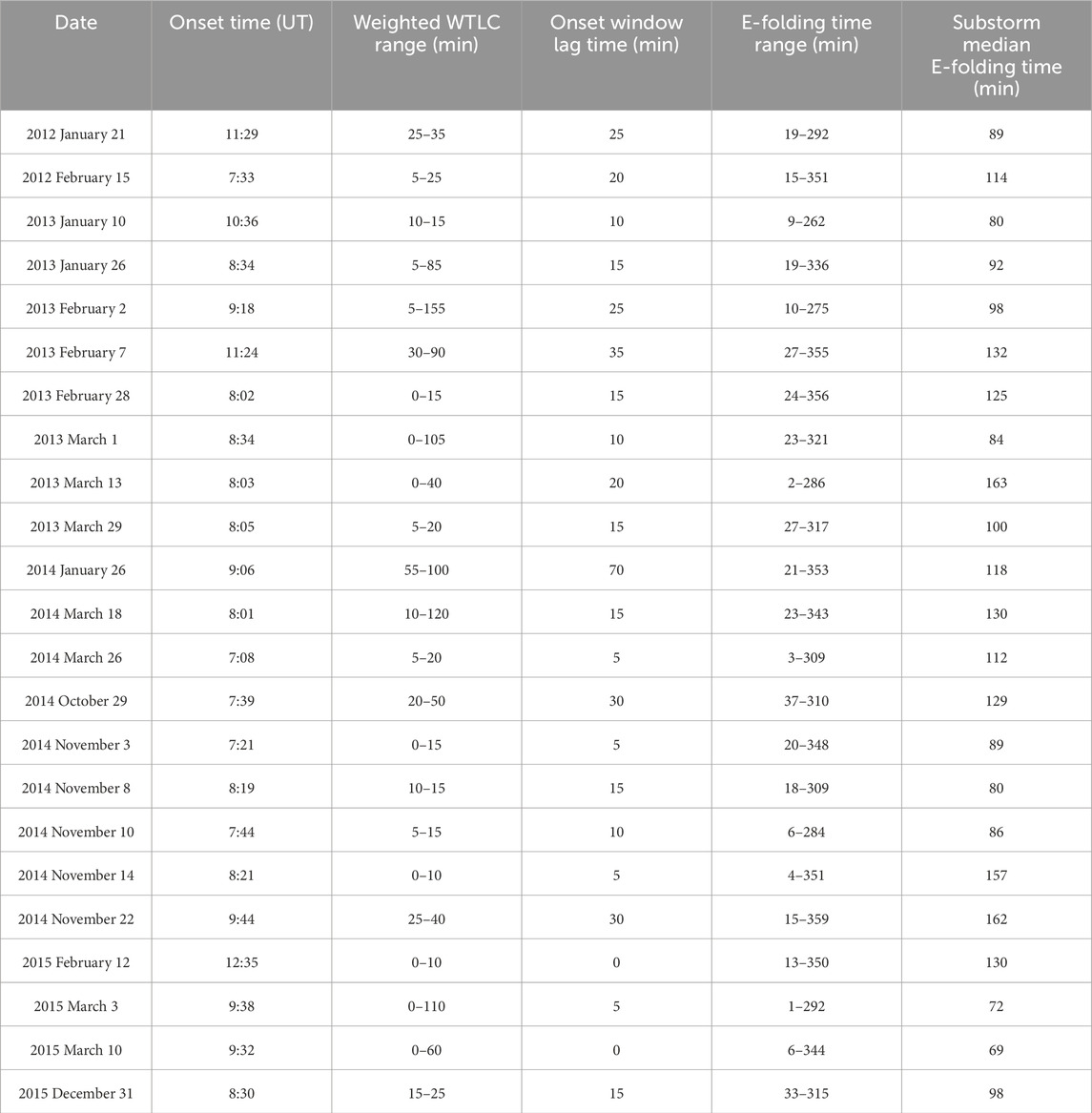
Table 1. Neutral wind response times of substorm events.

3.2 2014 March 18

An example of a substorm event with a relatively short neutral wind response time is shown in Figure 1. The left panel shows geomagnetic conditions, including the IMF $|$B$|$ and Bz component, the SYM/H index, the AE index, intensity keogram from the FYKN ASI, and long-pulse electron density from PFISR. The right panel shows the plasma and wind responses, including the zonal plasma flow keogram, zonal wind keogram, zonal plasma (solid blue curve) and wind (dashed red curve) time-series plot, and the weighted WTLC time. This event occurred on 2014 March 18, with substorm onset at 08:01 UT, 20.88 MLT and 67.65$°$ MLAT from the Newell and Gjerloev (2011) substorm list. The geomagnetic conditions of this event show a southward turning of IMF around 06:45 UT, 1 h and 15 min before substorm onset, with southward IMF maintained for a few hours after onset. IMF By is initially eastward, but begins turning westward around 1 h and 15 min before substorm onset, and remains westward for the duration of the event. The SYM-H index shows very weak or little enhancement of the ring current during this event (>−15 nT), indicating a quiet time substorm. The AE index was small leading up to substorm onset time (<200 nT) and rapidly increased to around 600 nT immediately following onset time. Auroral intensity data from the FYKN ASI shows a steady growth phase that expanded equatorward from around 71$°$ at 05:30 UT to around 66$°$ just before 08:00 UT. Equatorward brightening of the arc began around 7:15 UT, but poleward expansion did not occur until just before 08:00 UT. The electron density data shows a large electron density enhancement before 07:00 UT. This is most likely associated with daytime solar EUV ionization, which has been shown to enhance electron densities from around 8–20 MLT for the equinox months (Lovati et al., 2023; Kim et al., 2020; Cai et al., 2007). Local electron precipitation due to the substorm began around 7:30 UT above 300 km, extended down to around 150 km at substorm onset time, then receded back to higher altitudes after about 1 h. There was an additional large electron density enhancement extending between 300–500 km starting around 10:30 UT. However, this enhancement is outside the studied period of the substorm window and not applicable to the current study. In order to better quantify the electron densities during these events, we obtain a range of electron density by averaging the minimum five values and maximum five values in the 2 hour substorm window across the entire altitude FOV. This is done because the precipitation altitude range varies between events, and instead of subjectively selecting the precipitation altitude range, we average the bottom five and top five values to eliminate outliers that may be caused by the background electron density. The electron density for this event ranges from 2.60 x ${10}^8$ ${\text{m}}^{-3}$ to 2.71 x ${10}^{11}$ ${\text{m}}^{-3}$.

Figure 1

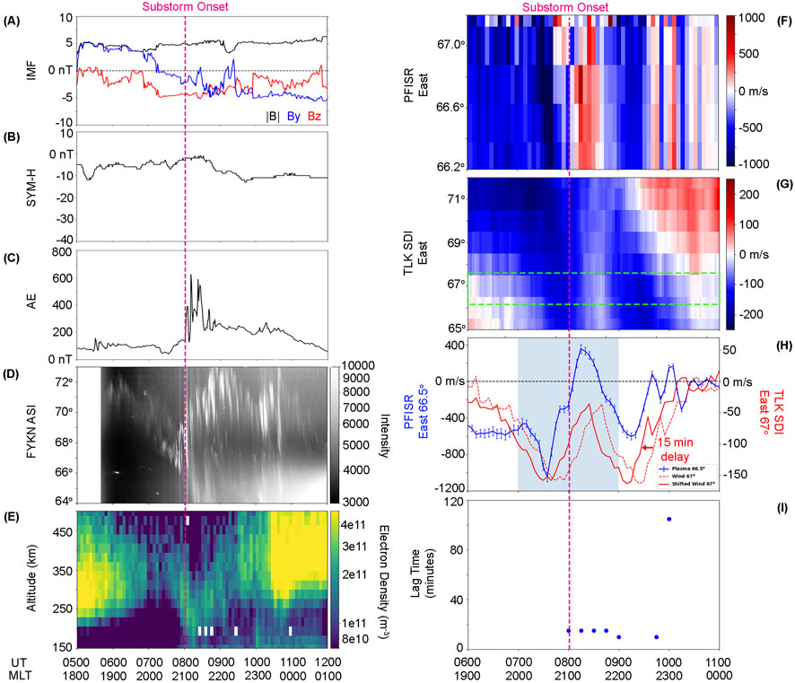
Figure 1. Summary of substorm event on 2014 March 18. Left panel (A–E) shows the IMF magnitude and southward component, the SYM/H index, the AE index, auroral keogram, and PFISR electron density. Right panel shows the (F,G) zonal plasma and wind velocity keograms, (H) zonal velocity time-series, with a dashed red line for the zonal wind and solid red line for the zonal wind shifted by the substorm window WWTLC time, and (I) the WWTLC response time vs. time. The magenta line in both the left and right panel indicates substorm onset. The green box in panel (G) highlights the PFISR FOV. The blue shading in panel (H) indicates the substorm window.

The plasma and neutral wind response to the substorm can be seen in the right panel of Figure 1. Figure 1F shows a keogram of the eastward component of the plasma’s horizontal velocity vector. The plasma flow was initially westward, and accelerated to a stronger westward flow around 7:00 UT. At around 7:30 UT, plasma accelerated eastward and reached a maximum eastward velocity at around 8:15 UT. Plasma turned westward again around 8:45 UT, and weakened to a near stagnant flow in the following 2 h. At substorm onset time, 8:01 UT, Poker Flat is roughly located around 21 MLT, placing our observations just eastward of the substorm onset location of 20.88 MLT. It has been shown that eastward of the substorm expansion phase auroral bulge, ionospheric currents are eastward (Gjerloev and Hoffman, 2001), which corresponds to the eastward plasma flow shown in this event. Figure 1G shows a keogram of the eastward neutral wind, extending from 65$°$ - 72$°$ MLAT. At around 71$°$ MLAT, the neutral wind reached a maximum westward velocity around 7:15 UT. Without larger FOV plasma data, which only covers around 66$°$ - 67$°$ MLAT in this case, it cannot be observed whether or not plasma is driving these westward accelerations. Although, based on the auroral keogram showing precipitation at these latitudes and studies that show ion-drag is a dominant neutral wind driver (Killeen and Roble, 1984), it is likely that this westward wind was associated with westward ionospheric plasma flows. The westward wind extended equatorward in time, with the entire latitude FOV showing westward wind starting around 7:30 UT. At the PFISR latitude range (66$°$ - 67$°$ MLAT), the wind accelerated eastward around substorm onset time, weakening the westward wind until it reached a minimum speed around 8:30 UT. The wind accelerated westward again, reaching a maximum speed around 9:30 UT, before stagnating around 10:30 UT.

The time-series of the zonal plasma and neutral wind velocity is shown in Figure 1H. The plasma flow is shown as a solid blue curve and the wind velocity is shown as a dashed red curve. The time-series data was taken from the keograms at the 66.5$°$ bin and 67$°$ bin, respectively. This data shows four acceleration periods of the plasma flow, similar to the observations in the keograms. There was an initial westward acceleration around 7:00 UT, an eastward acceleration around 7:30 UT, a westward acceleration around 8:15 UT, and a final eastward acceleration around 9:15 UT. The wind time-series data shows a very close following of this pattern, but with some of the accelerations delayed by around 15 min. The wind did not fully turn eastward at 8:30 UT like the plasma flow did, but that is because the plasma accelerated westward again before the wind could catch up to the eastward flow. Such close following of this acceleration pattern indicates a strong coupling between the plasma and the neutrals.

The calculated weighted WTLC neutral wind response times are shown in Figure 1I. The response time ranges from 10–105 min, although the 105 min response time corresponds to the last window of the event, where the plasma flow and wind have stagnated and therefore have less distinct features to match for the correlation calculation. The response time of the substorm window is 15 min, and the response time shortened to 10 min as the substorm progressed. The blue shaded region of Figure 1H shows the substorm window used for analysis. The solid red curve shows the wind shifted by 15 min, corresponding to the weighted WTLC time of the substorm window. This shift aligns the eastward acceleration of the wind to the eastward acceleration of the plasma at 7:30 UT as well as the westward accelerations at 8:15 UT. This analysis confirms the 15 min response time of the substorm window.

3.3 2014 November 22

An example of a substorm event with a relatively long neutral wind response time is shown in Figure 2. This event took place on 2014 November 22, with substorm onset at 09:44 UT, 21.22 MLT and 65.35$°$ MLAT from the Newell and Gjerloev (2011) substorm list. The geomagnetic conditions in the left panel of Figure 2 shows that IMF is mostly southward before the substorm, with some periodic reversals to northward IMF. IMF By experiences periodic reversals from eastward to westward prior to substorm onset, but is mostly weakly-directional from around 1 h before onset time to around 1 h after onset time. Around substorm onset time, IMF switched from southward to northward IMF and remains northward for around 2 h. The SYM/H index was slightly more enhanced for this event before onset time (<−20 nT), indicating more geomagnetic activity prior to the substorm. The SYM/H levels were still below that of a geomagnetic storm, however. The AE index was active before the substorm, fluctuating around 200–300 nT for around 4 h. At substorm onset time, the AE index increased to around 600 nT, but was not as sharp of an increase as the short response time substorm events. Auroral intensity data from the FYKN ASI keogram shows that auroral activity occurred a few hours before substorm onset, around 06:00 UT, but still show some poleward expansion of the auroral arc around 68$°$ MLAT at substorm onset. Electron density was slightly enhanced throughout the night, with larger enhancements starting around 08:30 UT at 250 km, where the plasma and neutral observations are. The electron density ranges from 1.17 x ${10}^8$ ${\text{m}}^{-3}$ to 4.08 x ${10}^{11}$ ${\text{m}}^{-3}$.

Figure 2

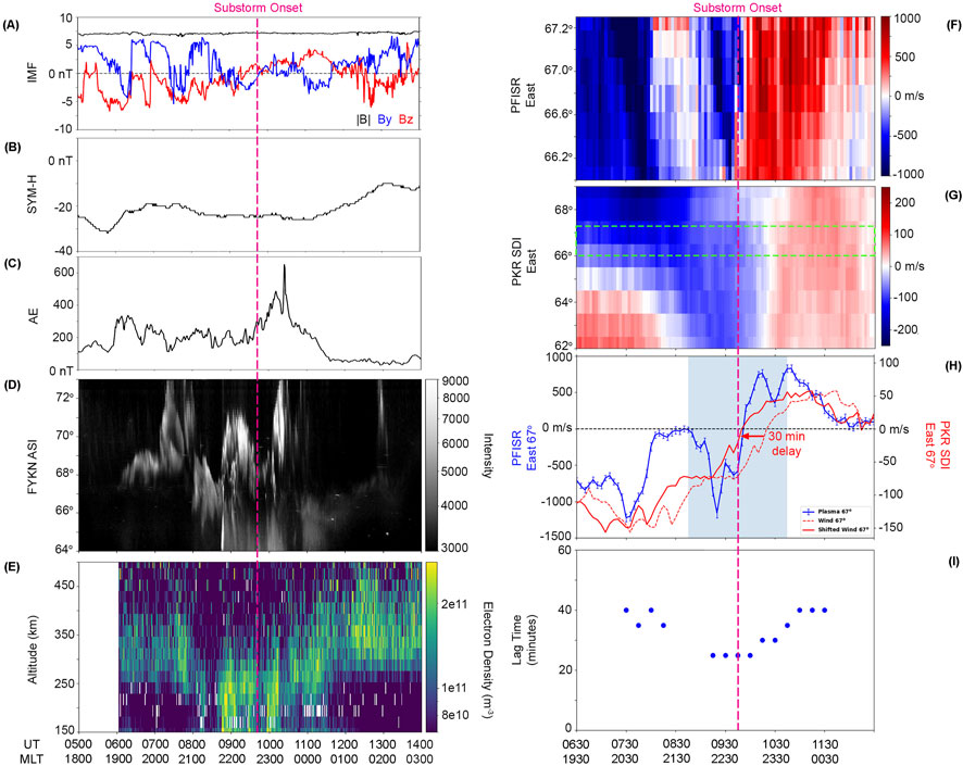
Figure 2. Summary of substorm event on 2014 November 22. Left panel (A–E) shows the IMF magnitude and southward component, the SYM/H index, the AE index, auroral keogram, and PFISR electron density. Right panel shows the (F,G) zonal plasma and wind velocity keograms, (H) zonal velocity time-series, with a dashed red line for the zonal wind and solid red line for the zonal wind shifted by the substorm window WWTLC time, and (I) the WWTLC response time vs. time. The magenta line in both the left and right panel indicates substorm onset. The green box in panel (G) highlights the PFISR FOV. The blue shading in panel (H) indicates the substorm window.

The plasma and neutral wind response can be seen in the right panel of Figure 2. Zonal plasma flow was initially strongly westward, then stagnated around 07:45 to 08:45 UT. At around 08:45 UT, the plasma became strongly westward again before quickly accelerating eastward, and became eastward flow by substorm onset time. This behavior was most likely due to multiple reconfigurations of ionospheric convection experienced during geomagnetically active periods, as we see AE activity enhancements before substorm onset. The zonal wind was initially westward above 65$°$ MLAT and eastward below 65$°$, indicating a strong wind shear at that latitude. The westward wind expanded equatorward, and the zonal wind became westward across all the entire FOV about 1 h before onset time, and shifted eastward around 45 min after substorm onset.

The time-series of the zonal plasma and wind velocity, taken at 67$°$ MLAT for both species (Figure 2H), exhibits the same behavior as described by the keograms. Both the plasma and the wind were initially westward. The plasma accelerated eastward around 07:30 UT into a stagnant flow between around 07:45–8:45 UT. The zonal wind also accelerated eastward at around 08:30 UT, and plateaued into a weaker westward wind between around 09:00 UT and 09:45 UT. This plateau likely occurred due to the lack of ionospheric forcing with a near 0 m/s flow. The plasma then began accelerating eastward around 9:15 UT, 30 min before onset time. The wind accelerated eastward around 09:45 UT, 30 min after the plasma eastward acceleration. This behavior indicates that the wind was following the plasma flow accelerations, but were clearly lagged behind by 30–45 min.

The calculated weighted WTLC response times in Figure 2I confirm the observational lag time estimate of the time-series, with neutral wind response times ranging from 25–40 min. The response time was longer before substorm onset, minimized around onset time, and then increased again. The response time of the substorm window was 30 min, as shown by the red solid curve in Figure 2I. This delay more closely matches the eastward accelerations of the plasma and the wind before substorm onset time. However, the shifted wind places the eastward acceleration just before (5 min) the eastward acceleration of the plasma, which is within the error limitations of the method laid out in Davidson et al. (2024). A 5 min error gives a substorm window response time of 25 min, which is still categorized as a long response event.

3.4 Superposed epoch analysis of geomagnetic conditions

The case studies showed clear differences in the geomagnetic conditions between the short and long response events. For the short response event, Bz turned southward around 1.5 h before substorm onset time. Meanwhile, the long response event showed Bz turning northward around 2 h before substorm onset time and was northward at substorm onset time. The short response event had a SYM/H index greater than −15 nT, consistent with a quiet-time substorm based on the storm time threshold of the SYM/H index (SYM/H ≤−80 nT (Hutchinson et al., 2011)). The long response event, however, occurred during a period of enhanced geomagnetic activity (SYM/H around −20 to −30 nT), although it is still beneath the threshold of a geomagnetic storm. This enhancement may exist because the event occurred during the recovery phase of a geomagnetic storm. Alternatively, frequent periods of southward IMF in the days prior to the event could have resulted in increased convection cycles and therefore more ring current injections. This is referred to as a geomagnetically active period for the remaining discussion. Additionally, the short response event exhibited no substorm activity prior to substorm onset, based on both the Newell and Gjerloev (2011) and Forsyth et al. (2015) substorm identification methods which both require a rapid decrease in the SML index for a sustained period of time. The long response event exhibited frequent enhancements, up to 400 nT, of the AE index prior to substorm onset time, indicating previous substorm activity. In order to better quantify these differences, and observe whether or not they are occurring on a statistical scale, a superposed epoch analysis (SEA) was performed of the geomagnetic conditions for the short and long response cases using the groupings discussed in Section 3.1. The SEA analysis $\pm$8 h from the SuperMAG substorm onset time.

The superposed epoch analysis was performed on IMF magnitude, By, Bz, AE index, and SYM/H index and is shown in Figure 3. The red line represents the SEA median, while the blue shaded region is the ${25}^{th}$ and ${75}^{th}$ percentile range. The short and long response SEA are shown in the left and right panel, respectively. The median IMF magnitude is similar between the short and long response events, with average median values of 5.80 nT and 6.90 nT, respectively. However, the range of the IMF magnitude is larger for the short responses events, with the maximum ${75}^{th}$ percentile value at 11.05 nT as compared to 9.22 nT for the long response events. The IMF By component has no strong directional trends for the short response events, with median values ranging from −2.20 nT to 1.91 nT and an average median value of −0.43 nT. The IMF By component for the long response events are mostly positive before substorm onset, with the median values ranging from −2.19 nT and 3.37 nT and an average median value of 1.26 nT. After substorm onset, the IMF By is weakly directional, with the median values ranging from −1.77 nT and 1.50 nT and an average median value of −0.03 nT. The percentile range, however, reaches more duskward values, reaching −7.35 nT after substorm onset as compared to −4.45 nT before substorm onset. However, these trends are weak and are most likely not the dominant component of the neutral wind response time.

Figure 3

Figure 3. Superposed epoch analysis of IMF $|$B$|$, By, Bz, AE and SYM/H index for the short (A–E) and long (F–J) response time events, where the epoch is the SuperMAG substorm onset time.

The trends in the IMF Bz component, the AE index, and the SYM/H index are more apparent. For the short response events, the median IMF Bz component turns southward 82.5 min before substorm onset, reaches a minimum value of −4.06 nT 7.5 min before onset time, and remains southward until 112.5 min after onset, where it becomes mostly non-directional for the remainder of the SEA time. The percentile range is small, with an average range of 4.44 nT, indicating that this trend is strong among all events. For the long response events, the median IMF Bz component is southward for the 8 h leading up to substorm onset time, with median values ranging from −5.32 nT and −1.50 nT. The median IMF Bz component does not turn northward again until 232.5 min after substorm onset time. Before substorm onset time, the percentile range is small, with an average range of 3.06 nT, indicating that the trend of sustained southward IMF prior to substorm onset for long response events is strong. After substorm onset, the IMF Bz component is more variable, with a larger average percentile range of 4.56 nT.

For the short response events, the median AE index is relatively weak leading up to onset time, ranging from 45.0 to 125.7 nT. The median AE index sharply increases to 288.3 nT 7.5 min after substorm onset time, then steadily decreases to its pre-substorm levels around 3.5–4.0 h after substorm onset. In the hours leading up to substorm onset time, the percentile range is very small, with the average range being 90.6 nT in the 247.5 min leading up to substorm onset. After substorm onset, the percentile range increases to an average range of 218.5 nT. This increase is most likely due to the varying strengths and recovery phases of the individual substorms. However, it is clear that quiet AE index conditions (<100 nT) prior to substorm onset is a strong trend for the short response events. For the long response events, the median AE index is more variable prior to substorm onset, ranging from 91.7 nT to 268.5 nT. At substorm onset time, the median AE index sharply increases, reaching a maximum of 353.7 nT 22.5 min after onset time. The median AE index then returns to quiet time values (<100 nT) around 4 h after onset time. The percentile range varies greatly before substorm onset time, with an average range of 185.2 nT and a maximum range of 415.2 nT. This indicates that while long response events generally have a more active AE index prior to substorm onset, the level of activity can vary between events. The average percentile range after substorm onset is 246.1 nT, more similar to the short response events and again indicating a variation in the individual substorm strengths and recovery.

For the short response events, the median SYM/H is relatively weak throughout the duration of the SEA time, ranging from −13.0 nT to 0.0 nT, and have no discernible trends around substorm onset time. The percentile range is relatively small, with an average range of 15.6 nT. For the long response events, the median SYM/H index is larger, ranging from −29.5 nT to −8.5 nT. The median SYM/H index is larger before substorm onset as compared to after substorm onset, with an average median of −23.2 nT (−14.9) before (after) onset time. The percentile range is also smaller before onset time, with an average range of 16 nT as compared to 26.8 nT after substorm onset.

The presence of southward IMF prior to substorm onset time allows for magnetic energy to load into the magnetotail, which is then unloaded at onset time. The loading process has been shown to last around 40 min once southward IMF begins (Nagai et al., 2005). Since the IMF for the short response events turn southward around 82.5 min before onset time, this would allow enough time to load the magnetotail for an energetic substorm. The long responses events experience southward IMF for many hours before substorm onset, and several loading and unloading cycles may occur during this time, potentially decreasing the amount of energy being stored and released upon each cycle since the unloading process does not require a minimum lobe flux growth (Nishimura and Lyons, 2021). This lower energy injection could result in slower neutral wind response times from having weaker ion-drag forcing. The trends in both the AE and SYM/H index indicate that neutral winds are more likely to respond quickly during geomagnetically quiet conditions, e.g., little to no variation in the AE index and AE index values of less than 100 nT and SYM/H index values greater than −20 nT. Conversely, the long response events are associated with heightened geomagnetic activity, e.g., variations in the AE index greater than 200 nT and SYM/H index values between −40 nT and −20 nT. These events may be compound substorm events or substorms that occur in the recovery phase of a geomagnetic storm, which would cause pre-substorm variations in the AE index and an enhanced SYM/H index. Studies have shown that compound substorm events increase the number of high-energy electrons in the precipitating particle population (Partamies et al., 2021), which would theoretically decrease the ion-neutral coupling time due to increased collisions. However, this result mainly impacts the lower E− and D-region ionosphere, and there have been few studies regarding the effects of compound substorms on F-region precipitation. Alternatively, studies have shown that wind speeds increase with increasing geomagnetic activity level (Omaya et al., 2023). A more perturbed initial state of the thermosphere could cause longer response times than a quiet initial state of the thermosphere, since the thermosphere is more massive and tends to keep its momentum, it would be more difficult for the ionosphere to change the direction of the thermosphere. Additionally, increased geomagnetic activity could result in thermospheric upwelling from Joule heating. An increase in thermospheric density at the F-region altitude could inhibit the ion-drag force, increasing the response time. Similarly, a study by Billett et al. (2020) has shown that E-region winds respond slower to changes in ionospheric convection during substorms as compared to F-region winds, most likely due to the higher density of the E-region. A more thorough analysis of the large-scale background thermospheric winds and density for these events are needed to determine the thermospheric pre-conditions impact on the neutral wind response time.

3.5 Superposed epoch analysis of electron density

Based on two case studies, differences in the electron density data are less obvious. The short response event had an electron density range from 2.60 x ${10}^8$ - 2.71 x ${10}^{11}$ ${\text{m}}^{-3}$, while the long response event had an electron density range from 1.17 x ${10}^8$ - 4.08 x ${10}^{11}$ m$-3$. While the long response event had a higher maximum electron density, these singular statistical values does not take into the consideration at what altitude or what time the electron density enhancement was in relation to substorm onset. For example, the electron density for the short response event maximizes around substorm onset time, while the long response event has periodic enhancements of the electron density throughout the event, and is not as coherent as the electron density profiles of the short response event. Again, in order to better quantify the trends in electron density between the short and long response events, a superposed epoch analysis was performed on the electron density profiles from PFISR. In order to capture the altitude variations in the electron density, a 2-dimensional epoch analysis was performed where the altitude was sorted into 15 km bins and the SEA was performed on each bin. The SEA is performed for $\pm$80 min from the SuperMAG substorm onset time. Two events were omitted from this analysis: 2014 March 26 and 2014 November 14. The 2014 March 26 event occurs close to the dayside electron density enhancement and biased the substorm electron density enhancements. The 2014 November 14 event did not have long-pulse data available for the F-region electron density.

The results of this SEA are shown in Figure 4, where the top and bottom panels shows the median electron density for the short and long response events, respectively. The electron density is larger for the short response events than for the long response events, ranging from 7.90 x ${10}^9$ - 2.03 x ${10}^{11}$ ${\text{m}}^{-3}$ with an average median of 9.14 x ${10}^{10}$ ${\text{m}}^{-3}$, as compared to 1.77 x ${10}^{10}$ - 1.90 x ${10}^{11}$ ${\text{m}}^{-3}$ with an average median of 8.27 x ${10}^{10}$ ${\text{m}}^{-3}$. Additionally, the electron density is larger in the 30 min leading up to and at substorm onset time for the short response events than for the long response events. From 32.5 min before to 2.5 min after substorm onset, the average median electron density is 9.15 x ${10}^{10}$ ${\text{m}}^{-3}$ for the short response events and 7.66 x ${10}^{10}$ ${\text{m}}^{-3}$ for the long response events. The pre-onset precipitation for the short response events could be due to precipitation during the growth phase of the substorm, which lasts around 1 h (Huang et al., 2003; Bargatze et al., 1999; McPherron et al., 1986). The long response events have electron density enhancements throughout the SEA time with no significant changes around substorm onset time. There is, however, an electron density enhancement around 15 min after onset time at 150 km. This altitude range is closer to the E-region ionosphere, and is outside the studied region. The electron density enhancements for the short response events are centralized between around 225–400 km before substorm onset, decreases to around 175–325 km at substorm onset time, and then increases its range again to 150–450 km after onset time. This behavior is an indication that the energy of the precipitation electrons increases at substorm onset, allowing the particles to penetrate further into the ionosphere. The 630.0 nm emissions of our observations are around 230 km (Sobral et al., 1993), which lies within the electron density enhancement region at substorm onset for the short response events. The long response events have electron density enhancements around 240–375 km for the duration of the SEA, with some enhancements below 175 km around 40–60 min before onset time and 15–80 min after onset time. These enhancements may be higher in altitude than our 630.0 nm emission observations, though the F-region can exist in a broad altitude range (150–400 km) and can vary in altitude during geomagnetically disturbed times (Yin et al., 2006). Therefore, some error can exist in the projected altitude of the F-region (Gillies et al., 2017), and more careful analysis is needed to determine whether or not these electron density enhancements exist within the observed altitude range.

Figure 4

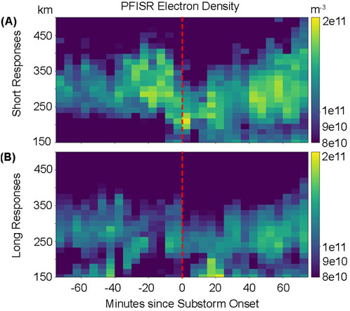
Figure 4. Superposed epoch analysis of PFISR’s long-pulse electron density data for the (A) short response and (B) long response events, where the epoch is the SuperMAG substorm onset time.

Some events not shown in this publication exhibited a delay in electron density from substorm onset time. One possible explanation is that the SuperMAG substorm lists rely on global indices to identify onset times and location. If PFISR is not located near the global onset location, this could result in delays in the local electron density enhancements while our observations move into the substorm electrojet region. To investigate this possibility, the THEMIS ground magnetometer station located at Poker Flat was utilized to identify the local perturbation onset time. For each event, the onset of perturbations in the northward component of the magnetic field was visually identified and then used as the epoch time in the electron density superposed epoch analysis. The perturbations of the northward component of the magnetic field represent the strength of the substorm electrojet, which is aligned east-west.

The results of this SEA are shown in Figure 5. The new local epoch times altered the spread of electron density enhancements in both the short and long response events. The short response events now show more consistent electron density enhancements throughout the SEA time, instead of being centralized around substorm onset time. The electron density is more enhanced in the 30 min after onset time than for the SuperMAG epoch time, with an average median of 9.16 x ${10}^{10}$ ${\text{m}}^{-3}$ for the local onset time as compared to 9.05 x ${10}^{10}$ ${\text{m}}^{-3}$ for the SuperMAG onset time from 2.5–37.5 min after epoch time. The long response events still do not show much variation of electron precipitation around onset time, though the electron density around 15 min before onset time is slightly larger, with the maximum median at 1.65 x ${10}^{11}$ ${\text{m}}^{-3}$ as compared to 1.46 x ${10}^{11}$ ${\text{m}}^{-3}$. The electron precipitation altitude range is similar for both epoch times for both the short and long response events. The electron density is still larger for the short response events than for the long response events, with an average median of nine. x25 x ${10}^{10}$ ${\text{m}}^{-3}$ as compared to 7.75 x ${10}^{10}$ ${\text{m}}^{-3}$ 22.5 min before and after local onset. The SEA using local magnetometer onset epoch times are subject to human error, since the perturbations were visually identified from the magnetometer data and could have an error of around 15 min. Future studies could apply the same methodologies as Newell and Gjerloev (2011) or Forsyth et al. (2015) to the local magnetometer data in order to better identify onset times. Considering this error, the results from the local onset epoch time and SuperMAG onset epoch time are similar, and that is that the electron density is higher for the short response events than for the long response events.

Figure 5

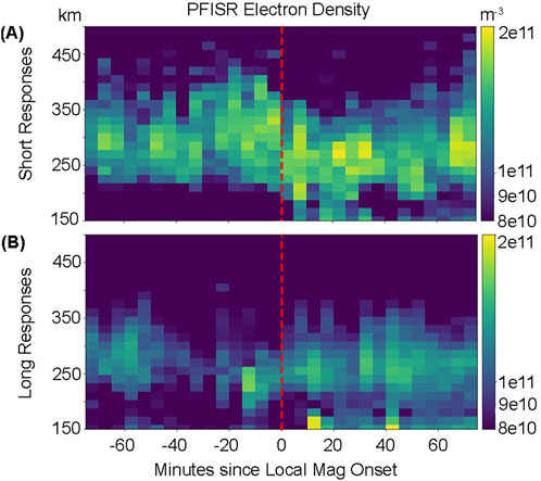
Figure 5. Superposed epoch analysis of PFISR’s long-pulse electron density data for the (A) short response and (B) long response events, where the epoch is the local magnetometer perturbation onset time.

The electron density profiles in the SEA show strong F-region enhancements of electron density for the short response events. While substorm precipitation typically occurs in the 557.0 nm green-line emission region (E-region), several studies show precipitation in the 630.0 nm red-line emission region (F-region) as well. A case study done by Liu et al. (2008) used the NORSTAR multispectral imager (MSI) and found equatorward moving streamers in the 630.0 nm emission line prior to substorm onset. Kepko et al. (2009) observed an equatorward moving diffuse auroral patch in the 630.0 nm emission line just before substorm onset. Gillies et al. (2017) used a REGO ASI and the Resolute Bay Incoherent Scatter Radar-Canadian (RISR-C) to study 630.0 nm auroral emissions and found that at the 220–240 km altitude range, electron density increased within red discrete arcs and in the region of diffuse aurora. This study also showed electron density enhancement in this altitude range, which produces more ion-neutral collisions and therefore a faster response time. Future work could include comparing the F-region density enhancements of our events to an ASI capable of observing the 630.0 nm emissions to see if the enhancements coincide with F-region auroral features.

It is important to note that the superposed epoch analyses are not a perfect representation of each short or long response event, but rather an average of the conditions of each group. Even though one event may share IMF characteristics with the short response group, it may share electron densities characteristics with the long response group, and vice versa. This result indicates that there is not one distinct controlling factor of the neutral wind response time. Neutral wind behavior is incredibly complex and, like the momentum equation shows, have many controlling factors. Even if neutral wind behavior were dependent on a single force, such as ion-drag, this force alone is dependent on plasma velocity, wind velocity, electron density, neutral density, and, to a lesser degree, ion and neutral temperatures. Because of this, a general characterization of the controlling factors of the neutral wind response time is difficult, and on a case by case basis more careful consideration should be used in order to pinpoint the controlling factors. However, this superposed epoch analysis is beneficial in a ‘more often than not’ approach. Because the SEA provides the average conditions of the short and long response events, we are able to say that more often than not, short and long neutral wind responses occur under those conditions.

3.6 Discussion of other controlling factors

Other controlling factors of the neutral wind response time have also been considered, such as the substorm onset time. Some events occur near magnetic midnight (0 MLT), which is around 11:00 UT for central Alaska. While this onset time falls within the typical MLT range of substorm onsets (Frey et al., 2004; Liou, 2010), winds in this region could also be subjected to strong anti-sunward forcing over the polar cap (Conde et al., 2001; Smith et al., 1998; Meriwether Jr. et al., 1988), potentially limiting it is response time to zonal forcing. Additionally, for earlier UT onset times, the central Alaska region could be spatially located further away from the typical near midnight substorm onset. For example, at 8:00 UT, central Alaska is around 20 MLT. This spatial separation could additionally hinder the neutral wind response time. However, Figure 6A shows the response time compared to UT onset time, and no clear dependence of UT is present. We also consider any seasonal dependence of the neutral wind response time. Dhadly et al. (2017) used 34 years of observational data to perform a climatological study of the large-scale neutral winds and found that mean neutral wind circulation increases from winter (Nov - Feb) to equinox (Mar, Apr, Sep, Oct) to summer (May - Aug) months. While this study has significantly less events than use in their study, we observe no seasonal dependence of the neutral wind response time, but no definitive conclusion can be made without a more robust data set. Consideration was also made for the SDI station used for each event. Since the study used both the Toolik Lake (68.6$°$N, −149.6$°$E) and Poker Flat (65.1$°$N, −147.5$°$E) SDIs, it is a possibility that the SDI location can influence the calculated neutral wind response times. Toolik Lake is about 2$°$ in longitude away from Poker Flat, where our plasma measurements are, meaning there could exist a spatial delay in the neutral wind response time, instead of a temporal delay. However, the SDI station used has little impact on the neutral wind response time, with 60% of short response events using TLK and 50% of long response events using TLK.

Figure 6

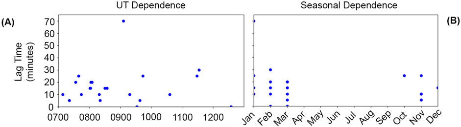
Figure 6. Neutral wind response time vs. (A) UT and (B) month.

Additional controlling factors include the presence of other thermospheric forces, such as pressure-gradient and advection forces. For example, the neutral winds may respond more slowly to ion-drag forcing if there exists a counteracting pressure-gradient force. Without more robust measurements of the high-latitude F-region thermosphere, it is difficult to estimate the influence of these forces. However, Davidson et al. (2025) showed that during active geomagnetic periods, ion-drag is a dominant zonal wind driver. Therefore, the addition of other forces may not have as strong of an influence on the neutral wind response time as the results of our SEA showed.

4 Summary

This study presented for the first time a statistical analysis of the neutral wind response time. The neutral wind response time is not well understood, and previous response time estimations range on the order of tens of minutes to hours, and are typically presented on a case by case basis. Using 23 substorm events, it was shown that statistically, F-region neutral wind response times are on the order of tens of minutes, with an average response time of $\sim$16 min. This result is similar to recent studies that have shown response times on the order of tens of minutes (Aruliah and Griffin, 2001; Anderson et al., 2011; Conde et al., 2018; Zou et al., 2018). A response time of this scale can quickly alter the mass distribution of the upper atmosphere, which is crucial for estimating the damaging effects of space weather such as satellite drag. Based on the average response time, events were split into short (≤15 min) and long (≥20 min) and a case study was shown for each category, including the geomagnetic and ionospheric conditions for each event. The short response case showed a southward turning of the IMF 1 h and 15 min before onset time, quiet SYM-H index conditions (>−15 nT) throughout the duration of the event, quiet AE index conditions (<200 nT) until substorm onset time, and electron density enhancement at substorm onset time. The long response event occurred during a period of heightened geomagnetic activity, with a slightly enhanced SYM-H index (between −20 and −40 nT) and AE index fluctuating around 200–300 nT for around 4 h before substorm onset time. The long response event also showed sustained southward IMF for around 5 h before substorm onset, but turned northward by onset time. Additionally, electron density enhancements were more sporadic for the long response event as compared to the short response event.

The case study analysis shows clear differences between short and long neutral wind response times, and a superposed epoch analysis was performed to observe whether or not these trends continued on a statistical scale. This analysis showed that more often than not, quiet-time conditions (the SYM/H index greater than −15 nT and the AE index of less than 200 nT with little variations) and a southward turning of IMF 82.5 min before substorm onset result in fast neutral wind response times. Alternatively, substorms that occur during more active periods (the SYM/H index between −20 and −40 nT and variations in the AE index up to 400 nT prior to substorm onset) are more likely to result in longer response times. These results suggest that geomagnetic pre-conditioning can affect the neutral atmosphere’s response to geomagnetic disturbances. For example, the southward turning of IMF around 1.5 h before substorm onset time for the short response cases would allow enough time for energy to be loaded into the magnetotail and released at onset time, whereas the sustained southward IMF of the long response events suggests multiple loading and unloading cycles, releasing less energy during the studied onset time. The effects of this pre-conditioning can be seen in the SEA of the electron density, which had higher amounts of precipitation for the short response events than for the long response events. The results of the electron density SEA indicate that larger ionospheric densities lead to a shorter neutral wind response time, due to the increased number of collisions and therefore stronger ion-drag forcing. These results also raise the question of the role of thermospheric pre-conditioning. The active geomagnetic conditions of the long response events could result in faster initial wind speeds and higher thermospheric densities, leading to longer response times. Further analysis is needed to investigate the role of thermospheric pre-conditioning, and this work is left for future studies.

In addition to the geomagnetic and ionospheric conditions, the neutral wind response time’s dependence on other controlling factors was investigated. The response time showed no dependence on UT, season, or SDI station being used for analysis. This study has shown that the controlling factors of the neutral wind response time are dynamic and dependent on the geomagnetic, ionospheric, and potentially thermospheric, pre-conditioning of disturbed times. While these factors may vary on a case to case basis, this study provides an average of the geomagnetic and ionospheric conditions of neutral wind responses.

Data availability statement

The datasets presented in this study can be found in online repositories. The names of the repository/repositories and accession number(s) can be found below: Data was made using a new package, which is now uploaded on https://zenodo.org/records/10892410. SDI data are available at http://sdi_server.gi.alaska.edu/sdiweb/index.asp. The THEMIS mission data are available from http://themis.ssl.berkeley.edu/index.shtml. PFISR operations data are available from http://amisr.com/database.

Author contributions

KD: Methodology, Conceptualization, Investigation, Writing – review and editing, Validation, Formal Analysis, Writing – original draft, Visualization, Funding acquisition. YZ: Supervision, Conceptualization, Writing – review and editing. LL: Writing – review and editing, Data curation, Writing – original draft. AB: Writing – review and editing, Data curation. MC: Data curation, Writing – review and editing.

Funding

The author(s) declare that financial support was received for the research and/or publication of this article. This work was supported by NASA grant 80NSSC21K1859. Publication fees were supported by the Department of Space Science, University of Alabama in Huntsville.

Acknowledgments

We acknowledge the SuperMAG collaborators (https://supermag.jhuapl.edu/info/?page%3Dacknowledgement). We acknowledge NASA contract NAS5-02099 and V. Angelopoulos for use of data from the THEMIS Mission. Specifically: S. Mende and E. Donovan for use of the ASI data, the CSA for logistical support in fielding and data retrieval from the GBO stations, and NSF for support of GIMNAST through grant AGS-1004736 and data provided by the Geophysical Institute Magnetometer Array operated by the Geophysical Institute, University of Alaska. More information about this dataset is available at http://magnet.asf.alaska.edu/. We acknowledge Poker Flat Incoherent Scatter Radar which is a major facility funded by the National Science Foundation through cooperative agreement AGS 1840962 to SRI International.

Conflict of interest

The authors declare that the research was conducted in the absence of any commercial or financial relationships that could be construed as a potential conflict of interest.

Generative AI statement

The author(s) declare that no Generative AI was used in the creation of this manuscript.

Publisher’s note

All claims expressed in this article are solely those of the authors and do not necessarily represent those of their affiliated organizations, or those of the publisher, the editors and the reviewers. Any product that may be evaluated in this article, or claim that may be made by its manufacturer, is not guaranteed or endorsed by the publisher.

References

Akasofu, S.-I. (1964). The development of the auroral substorm. Planet. Space Sci. 12, 273–282. doi:10.1016/0032-0633(64)90151-5

CrossRef Full Text | Google Scholar

Akasofu, S.-I. (2013). Where is the magnetic energy for the expansion phase of auroral substorms accumulated? J. Geophys. Res. Space Phys. 118, 7219–7225. doi:10.1002/2013JA019042

CrossRef Full Text | Google Scholar

Anderson, C., Conde, M., and McHarg, M. G. (2012a). Neutral thermospheric dynamics observed with two scanning Doppler imagers: 1. monostatic and bistatic winds. J. Geophys. Res. Space Phys. 117. doi:10.1029/2011JA017041

CrossRef Full Text | Google Scholar

Anderson, C., Conde, M., and McHarg, M. G. (2012b). Neutral thermospheric dynamics observed with two scanning Doppler imagers: 3. horizontal wind gradients. J. Geophys. Res. Space Phys. 117. doi:10.1029/2011JA017471

CrossRef Full Text | Google Scholar

Anderson, C., Davies, T., Conde, M., Dyson, P., and Kosch, M. J. (2011). Spatial sampling of the thermospheric vertical wind field at auroral latitudes. J. Geophys. Res. Space Phys. 116. doi:10.1029/.2011JA016485

CrossRef Full Text | Google Scholar

Aruliah, A. L., and Griffin, E. (2001). Evidence of meso-scale structure in the high-latitude thermosphere. Ann. Geophys. 19, 37–46. doi:10.5194/angeo-19-37-2001

CrossRef Full Text | Google Scholar

Bargatze, L. F., Ogino, T., McPherron, R. L., and Walker, R. J. (1999). Solar wind magnetic field control of magnetospheric response delay and expansion phase onset timing. J. Geophys. Res. Space Phys. 104, 14583–14599. doi:10.1029/1999JA900013

CrossRef Full Text | Google Scholar

Baron, M. J., and Wand, R. H. (1983). F region ion temperature enhancements resulting from joule heating. J. Geophys. Res. Space Phys. 88, 4114–4118. doi:10.1029/JA088iA05p04114

CrossRef Full Text | Google Scholar

Billett, D. D., McWilliams, K. A., and Conde, M. G. (2020). Colocated observations of the e and f region thermosphere during a substorm. J. Geophys. Res. Space Phys. 125, e2020JA028165. doi:10.1029/2020JA028165

CrossRef Full Text | Google Scholar

Cai, H. T., Ma, S. Y., Fan, Y., Liu, Y. C., and Schlegel, K. (2007). Climatological features of electron density in the polar ionosphere from long-term observations of eiscat/esr radar. Ann. Geophys. 25, 2561–2569. doi:10.5194/.angeo-25-2561-2007

CrossRef Full Text | Google Scholar

Cai, L., Oyama, S., Aikio, A., Vanhamäki, H., and Virtanen, I. (2019). Fabry-perot interferometer observations of thermospheric horizontal winds during magnetospheric substorms. J. Geophys. Res. Space Phys. 124, 3709–3728. doi:10.1029/2018JA026241

CrossRef Full Text | Google Scholar

Conde, M., Craven, J. D., Immel, T., Hoch, E., Stenbaek-Nielsen, H., Hallinan, T., et al. (2001). Assimilated observations of thermospheric winds, the aurora, and ionospheric currents over Alaska. J. Geophys. Res. Space Phys. 106, 10493–10508. doi:10.1029/2000JA000135

CrossRef Full Text | Google Scholar

Conde, M., and Smith, R. W. (1995). Mapping thermospheric winds in the auroral zone. Geophys. Res. Lett. 22, 3019–3022. doi:10.1029/95GL02437

CrossRef Full Text | Google Scholar

Conde, M., and Smith, R. W. (1997). Phase compensation of a separation scanned, all-sky imaging fabry–perot spectrometer for auroral studies. Appl. Opt. 36, 5441–5450. doi:10.1364/AO.36.005441

PubMed Abstract | CrossRef Full Text | Google Scholar

Conde, M., and Smith, R. W. (1998). Spatial structure in the thermospheric horizontal wind above poker flat, Alaska, during solar minimum. J. Geophys. Res. Space Phys. 103, 9449–9471. doi:10.1029/.97JA03331

CrossRef Full Text | Google Scholar

Conde, M. G., Bristow, W. A., Hampton, D. L., and Elliott, J. (2018). Multiinstrument studies of thermospheric weather above Alaska. J. Geophys. Res. Space Phys. 123, 9836–9861. doi:10.1029/2018JA025806

CrossRef Full Text | Google Scholar

Conde, M. G., and Nicolls, M. J. (2010). Thermospheric temperatures above poker flat, Alaska, during the stratospheric warming event of january and february 2009. J. Geophys. Res. Atmos. 115. doi:10.1029/2010JD014280

CrossRef Full Text | Google Scholar

Cousins, E. D. P., and Shepherd, S. G. (2010). A dynamical model of high-latitude convection derived from superdarn plasma drift measurements. J. Geophys. Res. Space Phys. 115. doi:10.1029/2010JA016017

CrossRef Full Text | Google Scholar

Davidson, K., Lu, G., and Conde, M. (2025). Effects of high-latitude input on neutral wind structure and forcing during the 17 march 2013 storm. J. Geophys. Res. Space Phys. 130, e2024JA033366. doi:10.1029/2024JA033366

CrossRef Full Text | Google Scholar

Davidson, K., Zou, Y., Conde, M., and Bhatt, A. (2024). A new method for analyzing f-region neutral wind response to ion convection in the nightside auroral oval. J. Geophys. Res. Space Phys. 129, e2024JA032415. doi:10.1029/2024JA032415

CrossRef Full Text | Google Scholar

Dhadly, M., Emmert, J., Drob, D., Conde, M., Doornbos, E., Shepherd, G., et al. (2017). Seasonal dependence of northern high-latitude upper thermospheric winds: a quiet time climatological study based on ground-based and space-based measurements. J. Geophys. Res. Space Phys. 122, 2619–2644. doi:10.1002/.2016JA023688

CrossRef Full Text | Google Scholar

Dhadly, M. S., Meriwether, J., Conde, M., and Hampton, D. (2015). First ever cross comparison of thermospheric wind measured by narrow- and wide-field optical Doppler spectroscopy. J. Geophys. Res. Space Phys. 120, 9683–9705. doi:10.1002/2015JA021316

CrossRef Full Text | Google Scholar

Forsyth, C., Rae, I. J., Coxon, J. C., Freeman, M. P., Jackman, C. M., Gjerloev, J., et al. (2015). A new technique for determining substorm onsets and phases from indices of the electrojet (sophie). J. Geophys. Res. Space Phys. 120 (10), 10592–10606. doi:10.1002/2015JA021343

CrossRef Full Text | Google Scholar

Frey, H. U., Mende, S. B., Angelopoulos, V., and Donovan, E. F. (2004). Substorm onset observations by image-fuv. J. Geophys. Res. Space Phys. 109. doi:10.1029/2004JA010607

CrossRef Full Text | Google Scholar

Fukizawa, M., Sakanoi, T., Ogawa, Y., Tsuda, T. T., and Hosokawa, K. (2021). Statistical study of electron density enhancements in the ionospheric f region associated with pulsating auroras. J. Geophys. Res. Space Phys. 126, e2021JA029601. doi:10.1029/.2021JA029601

CrossRef Full Text | Google Scholar

Gillies, M., Knudsen, D., Donovan, E., Jackel, B., Gillies, R., and Spanswick, E. (2017). Identifying the 630 nm auroral arc emission height: a comparison of the triangulation, fac profile, and electron density methods. J. Geophys. Res. Space Phys. 122, 8181–8197. doi:10.1002/2016JA023758

CrossRef Full Text | Google Scholar

Gjerloev, J. W., and Hoffman, R. A. (2001). The convection electric field in auroral substorms. J. Geophys. Res. Space Phys. 106, 12919–12931. doi:10.1029/1999JA000240

CrossRef Full Text | Google Scholar

Grandin, M., Partamies, N., and Virtanen, I. I. (2024). Statistical comparison of electron precipitation during auroral breakups occurring either near the open–closed field line boundary or in the central part of the auroral oval. Ann. Geophys. 42, 355–369. doi:10.5194/angeo-42-355-2024

CrossRef Full Text | Google Scholar

Heinselman, C. J., and Nicolls, M. J. (2008). A bayesian approach to electric field and e-region neutral wind estimation with the poker flat advanced modular incoherent scatter radar. Radio Sci. 43. doi:10.1029/.2007RS003805

CrossRef Full Text | Google Scholar

Huang, C.-S., Reeves, G. D., Borovsky, J. E., Skoug, R. M., Pu, Z. Y., and Le, G. (2003). Periodic magnetospheric substorms and their relationship with solar wind variations. J. Geophys. Res. Space Phys. 108. doi:10.1029/2002JA009704

CrossRef Full Text | Google Scholar

Hutchinson, J. A., Wright, D. M., and Milan, S. E. (2011). Geomagnetic storms over the last solar cycle: a superposed epoch analysis. J. Geophys. Res. Space Phys. 116. doi:10.1029/2011JA016463

CrossRef Full Text | Google Scholar

Jones, S. L., Lessard, M. R., Rychert, K., Spanswick, E., and Donovan, E. (2011). Large-scale aspects and temporal evolution of pulsating aurora. J. Geophys. Res. Space Phys. 116. doi:10.1029/.2010JA015840

CrossRef Full Text | Google Scholar

Kaeppler, S. R., Sanchez, E., Varney, R. H., Irvin, R. J., Marshall, R. A., Bortnik, J., et al. (2020). “Chapter 6 - incoherent scatter radar observations of 10–100kev precipitation: review and outlook,” in The dynamic loss of Earth’s radiation belts. Editors A. N. Jaynes, and M. E. Usanova (Elsevier), 145–197. doi:10.1016/.B978-0-12-813371-2.00006-8

CrossRef Full Text | Google Scholar

Kepko, L., Spanswick, E., Angelopoulos, V., Donovan, E., McFadden, J., Glassmeier, K.-H., et al. (2009). Equatorward moving auroral signatures of a flow burst observed prior to auroral onset. Geophys. Res. Lett. 36. doi:10.1029/2009GL041476

CrossRef Full Text | Google Scholar

Killeen, T. L., and Roble, R. G. (1984). An analysis of the high-latitude thermospheric wind pattern calculated by a thermospheric general circulation model: 1. momentum forcing. J. Geophys. Res. Space Phys. 89, 7509–7522. doi:10.1029/JA089iA09p07509

CrossRef Full Text | Google Scholar

Killeen, T. L., Won, Y.-I., Niciejewski, R. J., and Burns, A. G. (1995). Upper thermosphere winds and temperatures in the geomagnetic polar cap: solar cycle, geomagnetic activity, and interplanetary magnetic field dependencies. J. Geophys. Res. Space Phys. 100, 21327–21342. doi:10.1029/95JA01208

CrossRef Full Text | Google Scholar

Kim, E., Jee, G., Ji, E.-Y., Kim, Y., Lee, C., Kwak, Y.-S., et al. (2020). Climatology of polar ionospheric density profile in comparison with mid-latitude ionosphere from long-term observations of incoherent scatter radars: a review. J. Atmos. Solar-Terrestrial Phys. 211, 105449. doi:10.1016/j.jastp.2020.105449

CrossRef Full Text | Google Scholar

Kosch, M. J., Cierpka, K., Rietveld, M. T., Hagfors, T., and Schlegel, K. (2001). High-latitude ground-based observations of the thermospheric ion-drag time constant. Geophys. Res. Lett. 28, 1395–1398. doi:10.1029/.2000GL012380

CrossRef Full Text | Google Scholar

Lamarche, L. (2024). amisr/resolvedvelocities: v1.0.0-beta (v1.0.0-beta). doi:10.5281/zenodo.10892410

CrossRef Full Text | Google Scholar

Laundal, K. M., and Richmond, A. D. (2017). Magnetic coordinate systems. Space Sci. Rev. 206, 27–59. doi:10.1007/s11214-016-0275-y

CrossRef Full Text | Google Scholar

Liou, K. (2010). Polar ultraviolet imager observation of auroral breakup. J. Geophys. Res. Space Phys. 115. doi:10.1029/2010JA015578

CrossRef Full Text | Google Scholar

Liu, W. W., Liang, J., Donovan, E. F., Trondsen, T., Baker, G., Sofko, G., et al. (2008). Observation of isolated high-speed auroral streamers and their interpretation as optical signatures of Alfvén waves generated by bursty bulk flows. Geophys. Res. Lett. 35. doi:10.1029/2007GL032722

CrossRef Full Text | Google Scholar

Lovati, G., De Michelis, P., Alberti, T., and Consolini, G. (2023). Unveiling the core patterns of high-latitude electron density distribution at swarm altitude. Remote Sens. 15, 4550. doi:10.3390/rs15184550

CrossRef Full Text | Google Scholar

McPherron, R. L., Terasawa, T., and Nishida, A. (1986). Solar wind triggering of substorm expansion onset. J. geomagnetism Geoelectr. 38, 1089–1108. doi:10.5636/jgg.38.1089

CrossRef Full Text | Google Scholar

Mende, S. B., Harris, S. E., Frey, H. U., Angelopoulos, V., Russell, C. T., Donovan, E., et al. (2008). The themis array of ground-based observatories for the study of auroral substorms. Space Sci. Rev. 141, 357–387. doi:10.1007/s11214-008-9380-x

CrossRef Full Text | Google Scholar

Meriwether, Jr. J. W., Killeen, T. L., McCormac, F. G., Burns, A. G., and Roble, R. G. (1988). Thermospheric winds in the geomagnetic polar cap for solar minimum conditions. J. Geophys. Res. Space Phys. 93, 7478–7492. doi:10.1029/JA093iA07p07478

CrossRef Full Text | Google Scholar

Murr, D. L., and Hughes, W. J. (2001). Reconfiguration timescales of ionospheric convection. Geophys. Res. Lett. 28, 2145–2148. doi:10.1029/2000GL012765

CrossRef Full Text | Google Scholar

Nagai, T., Nakamura, R., Hori, T., and Kokubun, S. (2005). “The loading-unloading process in the magnetotail during a prolonged steady southward imf bz period,”. Frontiers in magnetospheric plasma Physics. Editors M. Hoshohino, Y. Omura, and L. Lanzerotti (Pergamon), 16, 190–193. doi:10.1016/S0964-2749(05)80029-0

CrossRef Full Text | Google Scholar

Newell, P. T., and Gjerloev, J. W. (2011). Evaluation of supermag auroral electrojet indices as indicators of substorms and auroral power. J. Geophys. Res. Space Phys. 116. doi:10.1029/2011JA016779

CrossRef Full Text | Google Scholar

Nishimura, Y., and Lyons, L. R. (2021). “The active magnetosphere,”. American Geophysical Union AGU, 277–291. chap. 18. doi:10.1002/9781119815624.ch18

CrossRef Full Text | Google Scholar

Omaya, S., Aikio, A., Sakanoi, T., Hosokawa, K., Vanhamaki, H., Cai, L., et al. (2023). Geomagnetic activity dependence and dawn-dusk asymmetry of thermospheric winds from 9-year measurements with a Fabry–Perot interferometer in Tromsø, Norway. Earth, Planets Space 75, 70. doi:10.1186/s40623-023-01829-0

CrossRef Full Text | Google Scholar

Oyama, S., Miyoshi, Y., Shiokawa, K., Kurihara, J., Tsuda, T. T., and Watkins, B. J. (2014). Height-dependent ionospheric variations in the vicinity of nightside poleward expanding aurora after substorm onset. J. Geophys. Res. Space Phys. 119, 4146–4156. doi:10.1002/2013JA019704

CrossRef Full Text | Google Scholar

Partamies, N., Tesema, F., Bland, E., Heino, E., Nesse Tyssøy, H., and Kallelid, E. (2021). Electron precipitation characteristics during isolated, compound, and multi-night substorm events. Ann. Geophys. 39, 69–83. doi:10.5194/angeo-39-69-2021

CrossRef Full Text | Google Scholar

Ponthieu, J.-J., Killeen, T. L., Lee, K. M., Carignan, G. R., Hoegy, W. R., and Brace, L. H. (1988). Ionosphere-thermosphere momentum coupling at solar maximum and solar minimum from de-2 and ae-c data. Phys. Scr. 37, 447–453. doi:10.1088/0031-8949/37/3/028

CrossRef Full Text | Google Scholar

Richmond, A. D. (1995). Ionospheric electrodynamics using magnetic apex coordinates. J. geomagnetism Geoelectr. 47, 191–212. doi:10.5636/jgg.47.191

CrossRef Full Text | Google Scholar

Richmond, A. D., Lathuillère, C., and Vennerstroem, S. (2003). Winds in the high-latitude lower thermosphere: dependence on the interplanetary magnetic field. J. Geophys. Res. Space Phys. 108. doi:10.1029/2002JA009493

CrossRef Full Text | Google Scholar

Rostoker, G., Akasofu, S.-I., Foster, J., Greenwald, R., Kamide, Y., Kawasaki, K., et al. (1980). Magnetospheric substorms—definition and signatures. J. Geophys. Res. Space Phys. 85, 1663–1668. doi:10.1029/JA085iA04p01663

CrossRef Full Text | Google Scholar

Russell, C. T., Chi, P. J., Dearborn, D. J., Ge, Y. S., Kuo-Tiong, B., Means, J. D., et al. (2009). THEMIS ground-based magnetometers. New York: Springer, 389–412. doi:10.1007/.978-0-387-89820-9_17

CrossRef Full Text | Google Scholar

Sánchez, E. R., Ruohoniemi, J. M., Meng, C.-I., and Friis-Christensen, E. (1996). Toward an observational synthesis of substorm models: precipitation regions and high-latitude convection reversals observed in the nightside auroral oval by dmsp satellites and hf radars. J. Geophys. Res. Space Phys. 101, 19801–19837. doi:10.1029/96JA00363

CrossRef Full Text | Google Scholar

Sangalli, L., Knudsen, D. J., Larsen, M. F., Zhan, T., Pfaff, R. F., and Rowland, D. (2009). Rocket-based measurements of ion velocity, neutral wind, and electric field in the collisional transition region of the auroral ionosphere. J. Geophys. Res. Space Phys. 114. doi:10.1029/2008JA013757

CrossRef Full Text | Google Scholar

Shumko, M., Chaddock, D., Gallardo-Lacourt, B., Donovan, E., Spanswick, E. L., Halford, A. J., et al. (2022). Aurorax, pyaurorax, and aurora-asi-lib: a user-friendly auroral all-sky imager analysis framework. Front. Astronomy Space Sci. 9. doi:10.3389/fspas.2022.1009450

CrossRef Full Text | Google Scholar

Smith, R. W., Hernandez, G., Roble, R. G., Dyson, P. L., Conde, M., Crickmore, R., et al. (1998). Observation and simulations of winds and temperatures in the antarctic thermosphere for august 2–10, 1992. J. Geophys. Res. Space Phys. 103, 9473–9480. doi:10.1029/97JA03336

CrossRef Full Text | Google Scholar

Sobral, J. H. A., Takahashi, H., Abdu, M. A., Muralikrishna, P., Sahai, Y., Zamlutti, C. J., et al. (1993). Determination of the quenching rate of the o(¹d) by o(³p) from rocket-borne optical (630 nm) and electron density data. J. Geophys. Res. Space Phys. 98, 7791–7798. doi:10.1029/92JA01839

CrossRef Full Text | Google Scholar

Spencer, E., Srinivas, P., and Vadepu, S. K. (2019). Global energy dynamics during substorms on 9 march 2008 and 26 february 2008 using satellite observations and the windmi model. J. Geophys. Res. Space Phys. 124, 1698–1710. doi:10.1029/2018JA025582

CrossRef Full Text | Google Scholar

Tanskanen, E., Pulkkinen, T. I., Koskinen, H. E. J., and Slavin, J. A. (2002). Substorm energy budget during low and high solar activity: 1997 and 1999 compared. J. Geophys. Res. Space Phys. 107, 15–11. doi:10.1029/2001JA900153

CrossRef Full Text | Google Scholar

Tanskanen, E. I. (2009). A comprehensive high-throughput analysis of substorms observed by image magnetometer network: years 1993–2003 examined. J. Geophys. Res. Space Phys. 114. doi:10.1029/.2008JA013682

CrossRef Full Text | Google Scholar

Wing, S., Gkioulidou, M., Johnson, J. R., Newell, P. T., and Wang, C.-P. (2013). Auroral particle precipitation characterized by the substorm cycle. J. Geophys. Res. Space Phys. 118, 1022–1039. doi:10.1002/jgra.50160

CrossRef Full Text | Google Scholar

Wing, S., Sibeck, D. G., Wiltberger, M., and Singer, H. (2002). Geosynchronous magnetic field temporal response to solar wind and imf variations. J. Geophys. Res. Space Phys. 107, 32–10. doi:10.1029/2001JA009156

CrossRef Full Text | Google Scholar

Yin, P., Mitchell, C., and Bust, G. (2006). Observations of the f region height redistribution in the storm-time ionosphere over europe and the USA using gps imaging. Geophys. Res. Lett. 33. doi:10.1029/2006GL027125

CrossRef Full Text | Google Scholar

Yu, Y., and Ridley, A. J. (2009). Response of the magnetosphere-ionosphere system to a sudden southward turning of interplanetary magnetic field. J. Geophys. Res. Space Phys. 114. doi:10.1029/2008JA013292

CrossRef Full Text | Google Scholar

Zou, Y., Lyons, L., Conde, M., Varney, R., Angelopoulos, V., and Mende, S. (2021). Effects of substorms on high-latitude upper thermospheric winds. J. Geophys. Res. Space Phys. 126, e2020JA028193. doi:10.1029/2020JA028193

CrossRef Full Text | Google Scholar

Zou, Y., Nishimura, Y., Lyons, L., Conde, M., Varney, R., Angelopoulos, V., et al. (2018). Mesoscale f region neutral winds associated with quasi-steady and transient nightside auroral forms. J. Geophys. Res. Space Phys. 123, 7968–7984. doi:10.1029/.2018JA025457

CrossRef Full Text | Google Scholar