Probing cosmic voids with emission-line galaxies

Introduction: We aim to provide forecasts for future line intensity mapping (LIM) observations and galaxy redshift surveys, focusing on the physical properties of low-density region of the cosmic web (voids). We study how the measured physical properties depend on the observational methods for void detection and identification.

Methods: We generate mock intensity maps targeting the far-infrared CO(3–2) emission line by assigning the line luminosities to dark matter halos in cosmological simulations. The popular void-finding algorithm VIDE is applied to identify cosmic voids and quantify their properties. We analyze the voids detected in two different observation modes: (1) three-dimensional galaxy redshift surveys and (2) two-dimensional LIM observations corresponding to a single-frequency bin at 173 GHz.

Results: We find that the measured void size functions and radial density profiles differ depending on the observational method. These features exhibit characteristic signatures that reflect both the underlying cosmology and the nature of the emission-line galaxies.

Discussion: LIM-based void detection is a promising avenue for cosmological studies. We discuss the potential of combining LIM and galaxy survey data in a joint analysis to improve constraints on cosmological parameters and to better understand emission-line galaxy populations.

1 Introduction

The large-scale structure (LSS) of the universe has been playing a critical role in modern cosmology. Statistical analysis of this LSS allows precise measurement of the geometry and energy content of the universe. Conventionally, photometric or spectroscopic galaxy surveys have been conducted to generate large-scale cosmic maps (Guzzo et al., 2018). Direct measurement or inference of the redshifts of a large number of galaxies is a costly process, and several years of operation of a large telescope is typically needed to complete a deep and wide-area survey of millions of galaxies.

Line intensity mapping (LIM) is an emerging observational technique for probing the distribution of galaxies in two and three dimensions in an efficient manner. LIM can be used to measure the collective intensity at a specific frequency from all emission sources, including those that have been redshifted on the frequency band. This feature enables detection of faint sources that cannot be identified individually, making LIM a unique method for probing the distribution of entire galaxy populations (Bernal and Kovetz, 2022; Kovetz et al., 2017). The large-scale matter distribution probing capacity of LIM offers invaluable opportunities for a wide range of studies in cosmology and fundamental physics. For example, it is possible to detect baryon acoustic oscillations and determine the expansion history of the universe through LIM observations (Karkare and Bird, 2018; Bernal et al., 2019). Multitracer LIMs enable placing tight constraints on the mass of the cosmic relic neutrino (Shmueli et al., 2025). LIM also provides a novel probe for small-scale clustering of dark matter (Muñoz et al., 2020) and hence its particle nature (Bauer et al., 2021; Sarkar et al., 2022).

Wideband or multifrequency LIM can be used to study the evolution of galaxies and history of cosmic star formation (Béthermin et al., 2022) through detection of a combination of various emission lines from hydrogen, carbon, and oxygen. LIM experiments in the far-infrared to millimeter range have allowed us to detect a set of molecular lines. Some of the ongoing and planned LIM experiments include CONCERTO (Van Cuyck et al., 2023), EXCLAIM (Ade et al., 2020), TIM (Vieira et al., 2020), and SUBLIME-TIFUUN (Kohno et al., 2024). The brand-new satellite SPHEREx is soon expected to provide near-infrared intensity maps for a very large area of the sky with high spectral resolution (Doré et al., 2014). Hence, it is important and timely to explore how we can use data from future observations for an array of studies in cosmology and astrophysics. In this work, we study the statistics of LSSs probed by CO(3-2) LIMs and galaxy surveys using mock observational data generated from cosmological simulations. In particular, we focus on cosmic voids and examine how they can be located in different types of observations. We first describe our method of void detection and then introduce a few basic statistics; then, we show the statistics derived from our simulations, followed by a discussion and some concluding remarks.

2 Galaxy distribution and LIM

We expect that the line intensities or intensity fluctuations reflect the underlying matter density fluctuations as

${\delta }_{\text{I}}\left(r,z\right)=\bar{I}\left(z\right)b\left(z\right){\delta }_{\text{m}}\left(r,z\right)+N\left(z\right),$

where ${\delta }_{\text{m}}(r,z)$ denotes the matter density fluctuation at position $(r,z)$, and $b(z)$ is the clustering bias of the galaxy population. The mean intensity $\bar{I}(z)$ represents the cumulative emission from all galaxies in the population.

There are already several successful observations of major line emissions from galaxies and the intergalactic medium. The HI intensity has been measured through cross-correlations between radio emissions and available galaxy redshift survey catalogs (Masui et al., 2013; Wolz et al., 2022). Other lines such as [CII] and CO emissions from high redshift have also been detected (Pullen et al., 2018; Yang et al., 2019). Low-density regions or cosmic voids can potentially be powerful probes for cosmology (Colberg et al., 2005). The abundant voids as functions of size (radius) and the density distribution within a void are believed to contain rich information on cosmology and the physics of galaxy formation. Galaxy surveys with sufficiently large effective volumes have been conducted only recently and have allowed measurements of the basic statistics of voids (Fernández-García et al., 2025). LIM is an efficient method for surveying a large volume and is also useful for considering multiple lines for detecting voids.

3 Methods

We used the Uchuu simulation (Ishiyama et al., 2021) to generate a three-dimensional galaxy distribution. The basic information regarding the Uchuu halo catalog used in this study is listed in Table 1. The halo catalogs were constructed using the ROCKSTAR halo finder and consistent-tree code (Behroozi et al., 2012a, 2012b) at redshift 1.0.

Table 1

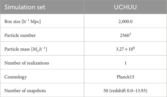
Table 1. Basic parameters for the Uchuu simulation.

Since the Uchuu simulation utilizes only one cosmological model, we used the COLA code¹ (Koda et al., 2016) to generate matter and halo distributions for different cosmologies. Herein, we briefly describe the mockups generated for this study.

$•$ Halo catalog

We generated a 3D halo catalog with a lower mass cutoff at $2\times 10^{12}{h}^{-1}{M}_{\odot }$ using COLA. Then, we adopted two cosmological models, where the one with ${\mathrm{\Omega }}_m=0.273,h_0=0.705,{\sigma }_8=0.812,{\mathrm{\Omega }}_{\mathrm{\Lambda }}=0.727$ was taken as the standard model and the other with ${\mathrm{\Omega }}_m=0.15,h_0=0.705,{\sigma }_8=0.812,{\mathrm{\Omega }}_{\mathrm{\Lambda }}=0.850$ was the small-Ω_m model. The box size was 500.0 h^–1 Mpc, number of N-body particles employed was 512³, and redshift was set at z = 0 for both realizations.

$•$ Dark energy spectroscopic instrument (DESI) mock

We generated a three-dimensional DESI mock catalog of [OII] emitting galaxies for DESI observation using the halo catalog of the Uchuu simulation. Here, we used halotool to populate galaxies in the dark matter halos using the halo occupation distribution (HOD) approach.

$•$ LIM mock

We generated LIM mocks using the halo catalogs generated by COLA. Here, we assumed the same two cosmological models as noted above, with the box size being 300.0 h^–1 Mpc, number of particles being 512³, and redshift being set to z = 1. We assigned the CO(3-2) line luminosity as a function of halo mass, whose details are further described in Section 3.2.

3.1 Mock DESI galaxies

We employ the HOD approach suitably calibrated to the [OII] emission-line galaxies (ELGs) observed by DESI (Rocher et al., 2024). We assume a Gaussian HOD model for the central galaxies with the expected occupation

$\langle N_{\text{cent}}\left(M\right)\rangle =\frac{A_{\text{c}}}{\sqrt{2\pi }{\sigma }_{\text{M}}}\cdot \exp \left[-\frac{{\left({\log }_{10}M-{\log }_{10}{M}_{\text{c}}\right)}^2}{2{\sigma }_{\text{M}}^2}\right]\equiv \langle N_{\text{cent}}^{\text{GHOD}}\left(M\right)\rangle$

and a power law model for the satellite galaxies with

$⟨N_{\text{sat}}\left(M\right)⟩=A_{\text{s}}{\left(\frac{M-M_0}{M_1}\right)}^{\alpha }.$

Here, A_c and A_s set the number density to match those of the observed galaxies; M_c is the typical halo mass to host the [OII] emitter as a central galaxy; ${\sigma }_{\text{M}}$ is the width of the Gaussian distribution. The low-mass cutoff M₀ determines whether a halo possesses a satellite galaxy, and α controls the halo mass dependence of the number of satellite galaxies. In this model, M₁ was introduced for normalization and is fixed at $10^{13}{h}^{-1}{\text{M}}_{\odot }$. The central galaxies are populated such that their positions and velocities match those of the halo centers. The satellite galaxies are distributed within a halo with a Navarro–Frenk and White profile (Navarro et al., 1996; Navarro et al., 1997)

$\rho \left(r\right)=\frac{{\rho }_{\text{s}}}{\frac{r}{r_{\text{s}}}{\left(1+\frac{r}{r_{\text{s}}}\right)}^2},$

where r is the distance from the halo center and r_s is the scale radius. The HOD parameters used in the present study are listed in Table 2.

Table 2

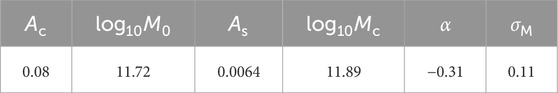
Table 2. Halo occupation distribution parameters used for DESI mock. The parameters were fitted against the clustering signal from the DESI 1 percent survey.

3.2 CONCERTO LIM mocks

We first generated 3D LIM mock catalogs using the COLA halo catalogs at redshift 1.0. It is expected that the star-forming galaxies at this redshift have strong CO(3-2) emissions as excellent targets for CONCERTO. We also included the interloper of CO(4-3) at redshift 1.67, which is redshifted to the same wavelength. Here, we briefly describe the method for assigning the CO(3-2) and CO(4-3) luminosities to each halo. First, we calculated the stellar mass of a halo using a double power-law stellar-to-halo mass ratio (SHMR) model proposed by Moster et al. (2010) as follows:

$\frac{M_{\ast }}{M_{\text{h}}}\left(z\right)=2A\left(z\right){\left[{\left(\frac{M_{\text{h}}}{M_{\text{A}}\left(z\right)}\right)}^{-\beta \left(z\right)}+{\left(\frac{M_{\text{h}}}{M_{\text{A}}\left(z\right)}\right)}^{\gamma \left(z\right)}\right]}^{-1}.$

We then use the best-fit parameters derived in Girelli et al. (2020) (A = 0.0353, log(M_A) = 12.05, β = 0.88, and γ = 0.599) with a 0.2 dex scatter. Next, we use an empirical relationship between the stellar mass and star formation rate (SFR) to calculate the infrared luminosity (Béthermin et al., 2022); in this procedure, we split the galaxies into star-forming and passive galaxies using the star-forming fraction given by Equation 1:

$f_{\text{SF}}\left(M_{\ast },z\right)=\left(1-f_{\text{Q},0}\left(z\right)\right)\frac{1-\text{erf}\left[\frac{{\log }_{10}\left(M_{\ast }\right)-{\log }_{10}\left(M_t\left(z\right)\right)}{{\sigma }_{\text{SF}}\left(z\right)}\right]}{2}(1)$

where $f_{Q,0}(z),M_t(z)$, and ${\sigma }_{\text{SF}}(z)$ denote the passive fractions of low-mass galaxies $(M_{\ast }\ll M_t(z))$, stellar mass threshold separating the star-forming and passive galaxies, and width of the transition as a function of the redshift.

The SFR of a galaxy is calculated using Equation 2:

$\begin{array}{cc}\hfill {\log }_{10}\left(\frac{\text{SFR}}{M_{\odot }/\text{yr}}\right)& ={\log }_{10}\left(\frac{M_{\ast }}{10^9{M}_{\odot }}\right)-m_0+a_0{\log }_{10}\left(z\right)\hfill \\ \hfill & -a_1{\left[\text{max}\left(0,{\log }_{10}\left(\frac{M_{\ast }}{10^9{M}_{\odot }}\right)-m_1-a_2{\log }_{10}\left(1+z\right)\right)\right]}^2.\hfill \end{array}(2)$

The infrared luminosity L_IR is calculated from the SFR using the Kennicutt (1998) conversion factor of $1.0\times 10^{-10}{M}_{\odot }/\text{yr}/L_{\odot }$. The CO(1-0) luminosity is then calculated from the L_IR using the empirical relationship of Equation 3 derived in Sargent et al. (2014):

${\log }_{10}\left(\frac{L_{\text{CO}\left(1-0\right)}^{\prime }}{\mathrm{K}\mathrm{k}\mathrm{m}{\mathrm{s}}^{-1}{\mathrm{p}\mathrm{c}}^2}\right)=0.81{\log }_{10}\left(\frac{L_{\text{IR}}}{L_{\odot }}\right)+0.54(3)$

The other transitions are calculated using the spectral line energy distribution template suggested by Bournaud et al. (2015). For the CO(4-3) interlopers, we generated a halo catalog at redshift 1.67 and calculated the CO(4-3) line luminosity using the steps described above. Since we expect that the CO(4-3) contaminants at z = 1.67 are not spatially correlated with the distribution of the CO(3-2) emitters at z = 1.0, we used a different random seed to generate the initial condition for the z = 1.67 halo catalog. We then downselect 20% of the halos by assuming that 80% of the interlopers can be removed using the methods discussed in Section 5. Although the contamination fraction is uncertain and arbitrary, we choose this value to quantify the impacts of the interlopers on void statistics.

We list the basic observational parameters used to generate the LIM catalog in Table 3; here, the parameters were set to closely follow the specifics of CONCERTO. We conducted the following analysis on a single slice of the LIM mock corresponding to an observer frame frequency of 173 GHz. Since we set the spectral resolution to 1 GHz and angular resolution to 32 arcsec, a single pixel in the 2D image included emissions from cubes of approximately 0.36 h^–1 Mpc width and 19.5 h^–1 Mpc depth for CO(3-2) emitters as well as 0.50 h^–1 Mpc width and 18.1 h^–1 Mpc depth for CO(4-3) emitters in the comoving space. We applied a minimum intensity threshold of 1 kJy/sr (corresponding to 0.52 K in brightness temperature) to remove low-intensity pixels with low signal-to-noise ratios in the actual observations and treated the pixels above this threshold as “signals” in the 2D maps.

Table 3

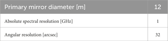
Table 3. Assumed observation specifications used to generate the LIM mocks.

3.3 Void detection

We located voids in the galaxy catalogs using a popular void finder called VIDE, whose full technical description is provided in Sutter et al. (2014); its applications in cosmology include cosmological parameter estimations using SDSS galaxies (Contarini et al., 2023) and constraints on neutrino masses (Bayer et al., 2024). Briefly, VIDE generates the Voronoi tessellation for a given particle (galaxy) distribution, where the density of each Voronoi cell is calculated as the inverse of its volume (or area in the 2D case). Cells that flow toward the same local density minimum are grouped together to form a zone; for each zone, the zone center is calculated as the volume-weighted center of all the particles in the zone, as shown in Equation 4:

${\mathbf{r}}_{\text{center}}=\frac{{\sum }_i{\mathbf{r}}_i{V}_i}{{\sum }_i{V}_i}.(4)$

The initial radius R_ini of each zone is calculated as the radius of a sphere (or circle in the 2D case) using the corresponding volume (area) of the detected zone, as shown in Equation 5:

$\begin{array}{cc}\hfill \frac{3}{4}\pi R_{\text{ini}}^3& ={\displaystyle \sum _i}{V}_i,\hfill \\ \hfill \pi R_{\text{ini}}^2& ={\displaystyle \sum _i}{V}_i.\hfill \end{array}(5)$

The central density of each zone is then calculated as the mean density within a spherical (circular) region around its center with a radius of 0.25R_ini. For direct comparisons with theoretical or analytic models, the zones are cleaned and rescaled as described in Jennings et al. (2013). The procedures are as follows:

$•$ Zones with central densities greater than $(1+{\delta }_{\nu }^{\text{NL}})\bar{\rho }$ will be removed from the void candidates. Here, $\bar{\rho }$ is the mean particle density and ${\delta }_{\nu }^{\text{NL}}$ is the non-linear density threshold for void detection. In our study, we used ${\delta }_{\nu }^{\text{NL}}=-0.7$ but note that the threshold can be set arbitrarily; however, the same threshold must be set for the theoretical prediction.

$•$ Starting from the zone center, we expanded the spherical (circular) region until the mean density reached the threshold of $(1+{\delta }_{\nu }^{\text{NL}})\bar{\rho }$. We then defined the radius of the sphere (circle) as the void radius.

$•$ For overlapping voids, we removed voids with higher central densities from the void list.

The void catalogs thus generated were used in the study subsequently.

4 Void statistics

4.1 Size function

One of the fundamental properties of a void is its size. Analogous to the halo mass function that characterizes the abundance of halos with different masses, the void size function describes the abundance of voids with different sizes and serves as a crucial statistical measure of the voids present in a large volume. A theoretical prediction of the void size function was provided by Sheth and van de Weygaert (2004) using the excursion-set approach (Press and Schechter, 1974), according to which the void size function in the linear regime is expressed by Equation 6:

${\left.\frac{dn}{d\ln r}\right|}_{\text{lin}}=\frac{f_{\ln \sigma }\left(\sigma \right)}{V\left(r\right)}\frac{d\ln {\sigma }^{-1}}{d\ln r}(6)$

where $f_{\ln \sigma }$ corresponds to the total area occupied by the voids, as defined by Equation 7:

$f_{\ln \sigma }\left(\sigma \right)=2{\displaystyle \sum _{j=1}^{\infty }}j\pi x^2\sin \left(j\pi \mathcal{D}\right)\exp \left[-\frac{{\left(j\pi x\right)}^2}{2}\right](7)$

Here, $\sigma$ is the square root of the mass variance, and x and D are defined by Equations 8, 9, respectively:

$x=\frac{\mathcal{D}}{|{\delta }_{\nu }^{\text{L}}|}(8)$

$\mathcal{D}=\frac{|{\delta }_{\nu }^{\text{L}}|}{{\delta }_c^{\text{L}}+|{\delta }_{\nu }^{\text{L}}|},(9)$

Here, ${\delta }_{\nu }^{\text{L}}$ is the under-density threshold to form voids, and ${\delta }_c^{\text{L}}$ is the over-density threshold to form halos, according to the excursion-set theory. The density threshold evolves with redshift according to Equation 10:

${\delta }^{\text{L}}\left(z\right)={\delta }^{\text{L}}\left(0\right)\frac{D\left(z\right)}{D\left(0\right)},(10)$

where $D(z)$ is the linear growth factor.

To predict the size function in a non-linear regime, we assume a volume-conserving model in which the total volume occupied by the voids is conserved within a single void-size bin. Under this assumption, the void size function can be rewritten as in Equation 11:

$\frac{dn}{d\ln r}={\left.\frac{dn}{d\ln r}\right|}_{\text{lin}}\frac{V\left(r_{\text{L}}\right)}{V\left(r\right)}\frac{d\ln r_{\text{L}}}{d\ln r},(11)$

where $r_{\text{L}}$ is the void radius defined in linear theory. The non-linear density threshold can be converted to its linear equivalent (Equation 12) using the fitting function derived in Bernardeau (1994). Thus,

${\delta }_{\nu }^{\text{L}}=\mathcal{C}\left[1-{\left(1+{\delta }_{\nu }^{\text{NL}}\right)}^{-1/\mathcal{C}}\right](12)$

with $\mathcal{C}=1.594$.

For biased tracers, the density threshold will also be biased, as shown in Equation 13:

${\delta }_{\nu ,\text{tr}}^{\text{NL}}=b_{\nu }{\delta }_{\nu }^{\text{NL}},(13)$

where $b_{\nu }$ corresponds to the tracer bias in the under-dense region. Its value can be directly calculated from the linear bias $b_{\text{eff}}$ using the empirical relation (Equation 14) derived in Contarini et al. (2019):

$b_{\nu }=\left(0.854\pm 0.007\right)b_{\text{eff}}+\left(0.420\pm 0.010\right).(14)$

Since we set our threshold as ${\delta }_{\nu ,\text{tr}}^{\text{NL}}=-0.7$, the linear density threshold used for the linear prediction is given by Equation 15:

${\delta }_{\nu }^{\text{L}}=1.594\left[1-0.3^{-1/1.594}\right]/b_{\nu }(15)$

Since the formation and evolution of voids are governed by the nature of dark energy and dark matter, the abundance of voids with different sizes is sensitive to the cosmological parameters (Li et al., 2012; Verza et al., 2019). Herein, we explore the size function of a void using different tracers and their dependence on the cosmological differences.

4.1.1 Void size function in galaxy distribution

We first calculated the void size functions for the halo catalog and DESI mock galaxies; here, we applied a low-mass cutoff at $2.0\times 10^{12}{h}^{-1}{M}_{\odot }$ for the halo catalog. Figure 1 shows the size functions of the voids detected from the halo catalog. The volume-conserving model prediction is remarkably well matched with the estimated void size function. We observed the detection of more voids with large radii and fewer voids with small radii for a smaller Ω_m. For a small Ω_m, the growth of high-density walls, which are the sheet-like structures surrounding the void regions, is suppressed; thus, smaller voids merge into larger voids before the surrounding walls start to collapse non-linearly.

Figure 1

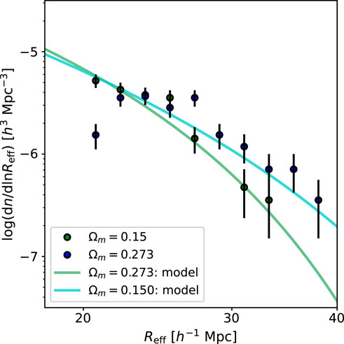
Figure 1. Size functions of voids detected from the halo catalog at different cosmology values: blue for Ω_m = 0.273 and green for Ω_m = 0.150. The plots show the size functions detected from the halo catalog, and the solid lines show the theoretical size functions calculated using the volume-conserving model of Equation 11. The error bars on the measured size functions are Poisson errors, assuming that the number of voids in each effective radius bin follows a Poisson distribution. We used decimal logarithmic void size bins ranging from 20 to 38 h^–1 Mpc.

Figure 2 shows the void size function detected using the DESI ELG mock catalog. The linear bias of b_eff = 1.273 was chosen to match the predicted linear bias from the angular correlation function of the DESI ELG targets (Kitanidis et al., 2020). Although the theoretical prediction slightly underestimated the abundance of small voids, the model was generally in good agreement with the detected void abundances. Therefore, the volume-conserving void size function model could be directly compared to the void abundances detected from the DESI ELGs.

Figure 2

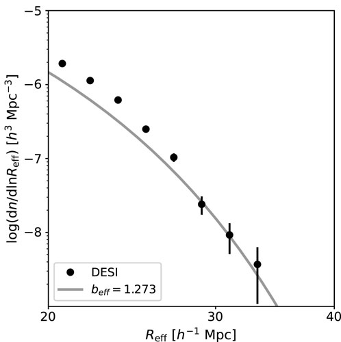
Figure 2. Size function of the voids detected from the DESI ELG mock catalog. The plot shows the size function detected from the halo catalog, and the solid line shows the theoretical prediction at redshift z = 1.0 with a linear bias of b_eff = 1.273. The error bars on the measured size function are Poisson errors, assuming that the number of voids in each effective radius bin follows a Poisson distribution. We used decimal logarithmic void size bins ranging from 20 to 38 h^–1 Mpc.

4.1.2 Void size function in LIM

Next, we calculates the size functions of the voids detected in LIM. Figure 3 shows the void size functions for our LIM mocks under different Ω_m. It is clear from the figure that the voids tend to be larger for smaller Ω_m, consistent with the results of the 3D galaxy distribution in the previous section. We expect that the void abundance in LIM could also serve as a cosmological probe, although further detailed modeling will be necessary for it to merit precision cosmology.

Figure 3

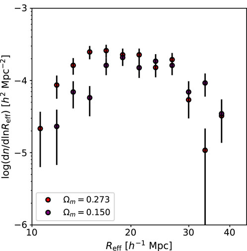
Figure 3. Size functions of voids detected from CO(3-2) LIM (without interlopers) at different cosmology values: red for Ω_m = 0.273 and purple for Ω_m = 0.150. The error bars on the measured size functions are Poisson errors, assuming that the number of voids in each effective radius bin follows a Poisson distribution. We used 12 logarithmic void size bins ranging from 10 to 40 h^–1 Mpc.

We also investigated the effects of the main interlopers, namely, CO (4-3) emitters, on the detected void abundance. Figure 4 shows the void size functions with and without the CO(4-3) interlopers. The interlopers tend to generate more small voids and fewer large voids. In general, adding random points can have two competing effects; large voids are separated into smaller voids owing to random points located inside the large voids, whereas the increase in mean density causes shallow voids to merge into larger voids. For the interlopers considered in this study, we only included 20% of the halos at z = 1.67, which means that the signal from the interlopers is typically smaller than the CO(3-2) signal. In this case, the change in mean density is negligible, and the first effect or increase in small void abundance is dominant.

Figure 4

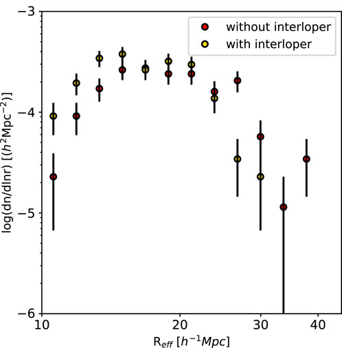
Figure 4. Size functions of voids detected from the LIM mock with (yellow) and without (red) the CO(4-3) interlopers. The error bars on the measured size functions are Poisson errors, assuming that the number of voids in each effective radius bin follows a Poisson distribution. We used 12 logarithmic void size bins ranging from 10 to 40 h^–1 Mpc.

4.2 Radial density profile

The radial profile of the voids is another important characteristic of the cosmic structure, which may be sensitive to clustering scales smaller than the free-streaming lengths of dark matter and relic neutrinos. In our study, we defined the radial profile of the voids in terms of particle density as a function of distance from the void center; here, the void center was defined as the centroid of the void region.

4.2.1 Radial density profile in galaxy distribution

We first calculated the void size functions for the halo catalog and DESI mock galaxies. Figure 5 shows the radial density profiles detected from the halo catalog with different cosmology values. We observed that for a fixed void radius, the stacked density profile did not change for different Ω_m. In general, the structures tended to become less clustered for lower Ω_m, so we expect that the density profiles of the voids would become weaker for lower Ω_m as well. However, since we are applying the same ${\delta }_{\nu }^{\text{NL}}=-0.7$ for both cosmologies, voids with weaker contrast merged to create a larger void. Therefore, if we compare the density profiles of voids at the same radius bin, there is no significant difference between them. By comparing the density profiles of voids with different sizes, we noted that the density contrast became slightly shallower for larger voids. This is in agreement with the results of a previous research by Hamaus et al. (2014), who studied the density profiles of voids using dark matter particles from N-body simulations.

Figure 5

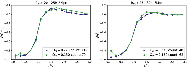
Figure 5. Stacked density profiles of voids detected from the halo catalog at different cosmology values: blue for Ω_m = 0.273 and green for Ω_m = 0.150. The y-axis represents the density normalized by the mean density, and the x-axis is the distance from the center normalized by the effective void radius. The two figures show the stacked density profiles of voids with different effective radii. In the left figure, we show the calculated density profiles of voids with effective radii of 20–25 h^–1 Mpc. The plots show the mean density profiles of all voids considered, and the error bars are the standard errors $\sigma /\sqrt{N}$. The figure on the right shows the calculated density profile for voids with effective radii of 25–30 h^–1 Mpc. We used 15 linear bins ranging from 0 to 3 for the normalized distance from the center. The numbers of voids included in the stacks are shown in the legends.

Figure 6 shows the radial density profiles detected from the DESI ELG mock catalog; comparing these with the void density profiles detected from the halo catalog, we note similar trends with void walls at around $r=r_{\text{v}}$ and the highest density peak at around $r=1.5r_{\text{v}}$. Comparing the density profiles for the same radius bin, we observe that the voids detected from the DESI mock are shallower than those detected from the halo mocks. This is attributed to the difference in redshift between the two mocks, with z = 0 for the halo catalog and z = 1 for the DESI mock. These results are also in agreement with the findings of Hamaus et al. (2014), who claimed that the density contrast would be weaker for a higher redshift that has a weaker structure than that of the low redshift.

Figure 6

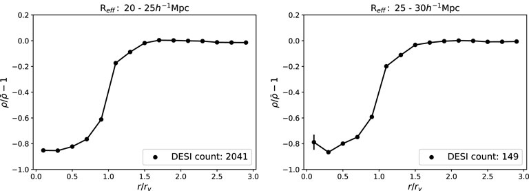
Figure 6. Stacked density profiles of voids detected from the DESI ELG mock catalog. The y-axis is the density-normalized by the mean density, and the x-axis is the distance from the center normalized by the effective void radius. The two figures show the stacked density profile of voids with different effective radii. In the left figure, we show the calculated density profile of voids with effective radii of 20–25 h^–1 Mpc. The plots show the mean density profiles of all voids considered, and the error bars show the standard errors $\sigma /\sqrt{N}$. We used 15 linear bins ranging from 0 to 3 for the normalized distance from the center. The figure on the right shows the calculated density profile for voids with effective radii of 25–30 h^–1 Mpc.

4.2.2 Radial density profile in LIM

Next, we calculated the radial density profiles of voids detected in the LIM mocks. We defined the radial density profile as the number density of pixels above the assumed luminosity threshold. Figure 7 shows the stacked density profiles of the voids detected for different mocks. Similar to the case of the 3D voids, the radial density profile is insensitive to differences in Ω_m. As with the trend for the 3D voids, we observed a steeper profile for the smaller voids. Compared to the voids detected in the 3D galaxy distribution, we argue that the LIM voids have higher density contrast and that the distances to the LIM void walls are less than the effective radius R_eff. These differences can be explained by the high tracer biases expected on the LIM mocks. We removed all pixels with intensities below 1 kJy/sr (0.52 K), which resulted in extremely low densities in the inner parts of the voids. Because there were fewer particles in the inner regions of the voids, the effective radii extended to the outer parts of the void walls to exceed the density threshold of ${\delta }_{\nu }^{\text{NL}}$. Moreover, some bright galaxies extended over multiple pixels owing to the beaming effect. In this case, multiple adjacent pixels that were separated by the pixel resolution (0.36 h^–1 Mpc) were included in the 2D point distribution. This manifests as an extremely high density in the void walls containing luminous tracers.

Figure 7

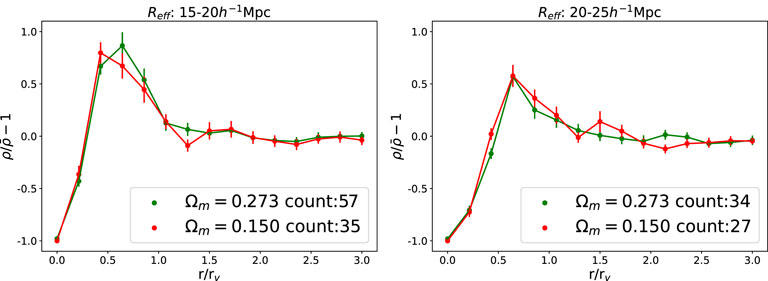
Figure 7. Stacked density profiles of voids detected from LIM at different cosmology values: green for Ω_m = 0.273 and red for Ω_m = 0.150. The y-axis is the density normalized by the mean density, and the x-axis is the distance from the center normalized by the effective void radius. The two figures show the stacked density profiles of voids with different effective radii. In the left figure, we show the calculated density profile of voids with effective radii of 15–20 h^–1 Mpc. The plots show the mean density profiles of all voids considered, and the error bars show the standard errors $\sigma /\sqrt{N}$. We used 15 linear bins ranging from 0 to 3 for the normalized distance from the center. The figure on the right shows the calculated density profile for voids with effective radii of 20–25 h^–1 Mpc. The numbers of voids included in the stacks are shown in the legends.

We also investigated how the interlopers affect the radial density profiles of the stacked voids. Figure 8 shows the radial density profiles of voids detected from LIM mocks with and without interlopers. The voids detected from the LIM mocks with interlopers tend to have shallower density profiles within $r_V$ compared to those without interlopers. This can be explained by two reasons. The first is that adding random points will increase the relative density of the low-density region, thereby decreasing the density contrast. The second is that “random” interlopers cause large voids to be separated into smaller voids. These small voids (which are actually parts of larger voids) tend to have smaller density contrast values compared to true voids and therefore render the radial density profile shallower.

Figure 8

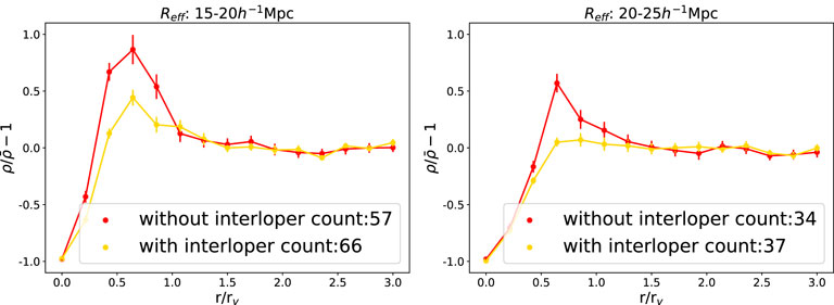
Figure 8. Stacked density profiles of voids detected from LIM mocks with (yellow) and without (red) the CO(4-3) interloper. The y-axis is the density normalized by the mean density, and the x-axis is the distance from the center normalized by the effective void radius. The two figures show the stacked density profiles of voids with different effective radii. In the left figure, we show the calculated density profiles of voids with effective radii of 15–20 h^–1 Mpc. The plots show the mean density profiles of all voids considered, and the error bars show the standard errors $\sigma /\sqrt{N}$. We used 15 linear bins ranging from 0 to 3 for the normalized distance from the center. The figure on the right shows the calculated density profiles for voids with effective radii of 20–25 h^–1 Mpc. The numbers of voids included in the stacks are shown in the legends.

5 Discussion and conclusion

We studied the properties of voids that will be observed in future galaxy surveys and LIM experiments. Using the mock observational catalogs generated from realistic cosmological simulations, we explored the size function and radial density profile as useful tools for characterizing large-scale mass distribution. The main results of this study are summarized as follows:

$•$ We showed that the void size function could be used as a cosmological probe. We also tested the applicability of the volume-conserving model for predicting the void size function.

$•$ By comparing the radial density profiles of different voids, we showed that differences in the cosmological parameter Ω_m do not significantly affect the corresponding density profiles.

$•$ We found similar features for voids detected from 2D LIM mock catalogs.

$•$ Interloper contamination tended to decrease the detected void size as well as the radial density contrast.

Based on our results, we conclude that the volume-conserving model is a good starting point for conducting cosmological analyses using void size functions derived from galaxy redshift surveys. In our analysis, we detected voids in real space and did not include the redshift space distortion effect, which will need to be accounted for in actual cosmological analyses. The peculiar velocities of the galaxies around voids are expected to vary for different Ω_m; thus, the radial density profiles in the redshift space may add additional information to the underlying matter distribution.

In this study, we confirmed the effects of interlopers and different cosmologies on the void properties. To conduct a cosmological forecast on future LIM observations, it is important to qualitatively evaluate the extents to which the void size functions and radial density profiles change under different cosmologies. These considerations along with more realistic observational effects, such as the foreground, are intended as our next step toward utilizing void properties to constrain cosmological models using LIM. Interestingly, state-of-the-art cosmological simulations have shown that galaxies residing in void regions, which are often referred to as void galaxies, have distinct properties over their counterparts residing in high-density regions (Rosas-Guevara et al., 2022). Therefore, the radial luminosity profiles of LIM voids could add information to the galaxy evolution model in the low-density regions. In this context, predictions using high-precision simulations for modeling radiation while accounting for environmental effects and mergers are required.

In the present study, we considered a simple interloper model in which 20% of the halos at z = 1.67 contaminate the intensity in the 173 GHz bin after the cleaning procedure. There are several approaches to mitigate interloper contamination. One such method is to perform component separation together with noise reduction and foreground removal, while another method may be to perform an end-to-end simulation so that the mock intensity catalogs also include multiple emission lines from galaxies at different redshift values. Several practical techniques have been proposed in this regard. Component separation is essential for detecting and characterizing voids, as we have explored herein; machine learning could be a powerful tool for this purpose (Moriwaki et al., 2020). Joint analysis of the galaxy surveys and LIM could also be a powerful tool for mitigating the effects of interlopers. Since the two sets of observations probe the same density fluctuations, the detected void distributions should have a positive correlation. Therefore, comparing the void properties from the two sets of observations is a powerful and robust analytical approach against interlopers.

The multiwavelength feature of upcoming LIM projects and its sensitivity to faint galaxies make LIM a powerful tool for understanding the evolution of galaxies and history of star formation. By investigating multiple emission lines, we expect to be able to probe multiple populations and gas phases of the galaxies. In this study, we did not assume any relationship between the line intensities and surrounding environments. However, by comparing the intensity profiles of void regions detected from observations and mocks including interactions between the LSSs, we expect to achieve a better understanding of how the surrounding environment affects the evolution of a galaxy. LIM experiments deliver massive amounts of data that include information on both the physical and frequency domains. Hence, it is important to consider the concerted use of theory, computations, data science, and artificial-intelligence-assisted studies (Moriwaki et al., 2023).

Data availability statement

The raw data supporting the conclusions of this article will be made available by the authors without undue reservation.

Author contributions

YY: conceptualization, investigation, methodology, and writing – original draft. NY: funding acquisition, methodology, supervision, writing – original draft, and writing – review and editing.

Funding

The author(s) declare that financial support was received for the research and/or publication of this article. The authors acknowledge financial support from the JSPS Kakenhi International Leading Research (no. 23K20035).

Acknowledgments

The authors thank Kana Moriwaki and Adrian Bayer for the insightful discussions. This research was supported by the Forefront Physics and Mathematics Program to Drive Transformation (FoPM), a WISE Program (Doctoral Program for World-Leading Innovative and Smart Education) at the University of Tokyo supported by MEXT, Japan. The authors also acknowledge the support of the Tokyo–Princeton Strategic Partnership for promoting academic exchange and collaboration.

Conflict of interest

The authors declare that the research was conducted in the absence of any commercial or financial relationships that could be construed as a potential conflict of interest.

Generative AI statement

The author(s) declare that no Generative AI was used in the creation of this manuscript.

Publisher’s note

All claims expressed in this article are solely those of the authors and do not necessarily represent those of their affiliated organizations, or those of the publisher, the editors and the reviewers. Any product that may be evaluated in this article, or claim that may be made by its manufacturer, is not guaranteed or endorsed by the publisher.

Footnotes

¹COLA is a fast cosmological N-body simulation code using the COmoving Lagrangian Acceleration technique (Tassev et al., 2013).

References

Ade, P. A. R., Anderson, C. J., Barrentine, E. M., Bellis, N. G., Bolatto, A. D., Breysse, P. C., et al. (2020). The experiment for cryogenic large-aperture intensity mapping (EXCLAIM). J. Low Temp. Phys. 199, 1027–1037. doi:10.1007/s10909-019-02320-5

CrossRef Full Text | Google Scholar

Bauer, J. B., Marsh, D. J. E., Hložek, R., Padmanabhan, H., and Laguë, A. (2021). Intensity mapping as a probe of axion dark matter. Mon. Not. R. Astron. Soc. 500, 3162–3177. doi:10.1093/mnras/staa3300

CrossRef Full Text | Google Scholar

Bayer, A. E., Liu, J., Kreisch, C. D., and Pisani, A. (2024). Significance of void shape: neutrino mass from Voronoi void halos? Phys. Rev. D. 110, L061305. doi:10.1103/PhysRevD.110.L061305

CrossRef Full Text | Google Scholar

Behroozi, P. S., Wechsler, R. H., and Wu, H.-Y. (2012a). The rockstar phase-space temporal halo finder and the velocity offsets of cluster cores. Astrophys. J. 762, 109. doi:10.1088/0004-637x/762/2/109

CrossRef Full Text | Google Scholar

Behroozi, P. S., Wechsler, R. H., Wu, H.-Y., Busha, M. T., Klypin, A. A., and Primack, J. R. (2012b). Gravitationally consistent halo catalogs and merger trees for precision cosmology. Astrophys. J. 763, 18. doi:10.1088/0004-637x/763/1/18

CrossRef Full Text | Google Scholar

Bernal, J. L., Breysse, P. C., and Kovetz, E. D. (2019). Cosmic expansion history from line-intensity mapping. Phys. Rev. Lett. 123, 251301. doi:10.1103/PhysRevLett.123.251301

PubMed Abstract | CrossRef Full Text | Google Scholar

Bernal, J. L., and Kovetz, E. D. (2022). Line-intensity mapping: theory review with a focus on star-formation lines. Astron. Astrophys. Rev. 30, 5. doi:10.1007/s00159-022-00143-0

CrossRef Full Text | Google Scholar

Bernardeau, F. (1994). The nonlinear evolution of rare events. Astrophys. J. 427, 51. doi:10.1086/174121

CrossRef Full Text | Google Scholar

Béthermin, M., Gkogkou, A., Van Cuyck, M., Lagache, G., Beelen, A., Aravena, M., et al. (2022). CONCERTO: high-fidelity simulation of millimeter line emissions of galaxies and [CII] intensity mapping. Astron. Astrophys. 667, A156. doi:10.1051/0004-6361/202243888

CrossRef Full Text | Google Scholar

Bournaud, F., Daddi, E., Weiß, A., Renaud, F., Mastropietro, C., and Teyssier, R. (2015). Modeling CO emission from hydrodynamic simulations of nearby spirals, starbursting mergers, and high-redshift galaxies. Astron. Astrophys. 575, A56. doi:10.1051/0004-6361/201425078

CrossRef Full Text | Google Scholar

Colberg, J. M., Sheth, R. K., Diaferio, A., Gao, L., and Yoshida, N. (2005). Voids in a ΛCDM universe. Mon. Not. R. Astron. Soc. 360, 216–226. doi:10.1111/j.1365-2966.2005.09064.x

CrossRef Full Text | Google Scholar

Contarini, S., Pisani, A., Hamaus, N., Marulli, F., Moscardini, L., and Baldi, M. (2023). Cosmological constraints from the BOSS DR12 void size function. Astrophys. J. 953, 46. doi:10.3847/1538-4357/acde54

CrossRef Full Text | Google Scholar

Contarini, S., Ronconi, T., Marulli, F., Moscardini, L., Veropalumbo, A., and Baldi, M. (2019). Cosmological exploitation of the size function of cosmic voids identified in the distribution of biased tracers. Mon. Not. R. Astron. Soc. 488, 3526–3540. doi:10.1093/mnras/stz1989

CrossRef Full Text | Google Scholar

Doré, O., Bock, J., Ashby, M., Capak, P., Cooray, A., de Putter, R., et al. (2014). Cosmology with the SPHEREX all-sky spectral survey. arXiv. doi:10.48550/arXiv.1412.4872

CrossRef Full Text | Google Scholar

Fernández-García, E., Betancort-Rijo, J. E., Prada, F., Ishiyama, T., Klypin, A., and Ereza, J. (2025). Constraining cosmological parameters using void statistics from the SDSS survey. Astron. Astrophys. 695, A19. doi:10.1051/0004-6361/202451264

CrossRef Full Text | Google Scholar

Girelli, G., Pozzetti, L., Bolzonella, M., Giocoli, C., Marulli, F., and Baldi, M. (2020). The stellar-to-halo mass relation over the past 12 gyr: I. standard cdm model. Astron. Astrophys. 634, A135. doi:10.1051/0004-6361/201936329

CrossRef Full Text | Google Scholar

Guzzo, L., Bel, J., Bianchi, D., Carbone, C., Granett, B. R., Hawken, A. J., et al. (2018). Measuring the Universe with galaxy redshift surveys. arXiv, 1–16. doi:10.1007/978-3-030-01629-6_1

CrossRef Full Text | Google Scholar

Hamaus, N., Sutter, P. M., and Wandelt, B. D. (2014). Universal density profile for cosmic voids. Phys. Rev. Lett. 112, 251302. doi:10.1103/physrevlett.112.251302

PubMed Abstract | CrossRef Full Text | Google Scholar

Ishiyama, T., Prada, F., Klypin, A. A., Sinha, M., Metcalf, R. B., Jullo, E., et al. (2021). The Uchuu simulations: data Release 1 and dark matter halo concentrations. Mon. Not. R. Astron. Soc. 506, 4210–4231. doi:10.1093/mnras/stab1755

CrossRef Full Text | Google Scholar

Jennings, E., Li, Y., and Hu, W. (2013). The abundance of voids and the excursion set formalism. Mon. Not. R. Astron. Soc. 434, 2167–2181. doi:10.1093/mnras/stt1169

CrossRef Full Text | Google Scholar

Karkare, K. S., and Bird, S. (2018). Constraining the expansion history and early dark energy with line intensity mapping. Phys. Rev. D. 98, 043529. doi:10.1103/PhysRevD.98.043529

CrossRef Full Text | Google Scholar

Kennicutt, R. C. (1998). The global Schmidt law in star-forming galaxies. Astrophys. J. 498, 541–552. doi:10.1086/305588

CrossRef Full Text | Google Scholar

Kitanidis, E., White, M., Feng, Y., Schlegel, D., Guy, J., Dey, A., et al. (2020). Imaging systematics and clustering of desi main targets. Mon. Not. R. Astron. Soc. 496, 2262–2291. doi:10.1093/mnras/staa1621

CrossRef Full Text | Google Scholar

Koda, J., Blake, C., Beutler, F., Kazin, E., and Marin, F. (2016). Fast and accurate mock catalogue generation for low-mass galaxies. Mon. Not. R. Astron. Soc. 459, 2118–2129. doi:10.1093/mnras/stw763

CrossRef Full Text | Google Scholar

Kohno, K., Endo, A., Tamura, Y., Taniguchi, A., Takekoshi, T., Ikeda, S., et al. (2024). “Sub/millimeter-Wave dual-band line intensity mapping using the terahertz integral field units with universal nanotechnology (TIFUUN) for the atacama submillimeter telescope experiment (ASTE),” in Millimeter, submillimeter, and far-infrared detectors and instrumentation for astronomy XII. Editors J. Zmuidzinas, and J.-R. Gao (Bellingham, United States: International Society for Optics and Photonics SPIE), PC13102. doi:10.1117/12.3021109

CrossRef Full Text | Google Scholar

Kovetz, E. D., Viero, M. P., Lidz, A., Newburgh, L., Rahman, M., Switzer, E., et al. (2017). Line-intensity mapping: 2017 status report. Report.

Google Scholar

Li, B., Zhao, G.-B., and Koyama, K. (2012). Haloes and voids in f(r) gravity: haloes and voids in f(r) gravity. Mon. Not. R. Astron. Soc. 421, 3481–3487. doi:10.1111/j.1365-2966.2012.20573.x

CrossRef Full Text | Google Scholar

Masui, K. W., Switzer, E. R., Banavar, N., Bandura, K., Blake, C., Calin, L. M., et al. (2013). Measurement of 21 cm brightness fluctuations at z ˜0.8 in cross-correlation. Astrophys. J. 763, L20. doi:10.1088/2041-8205/763/1/L20

CrossRef Full Text | Google Scholar

Moriwaki, K., Filippova, N., Shirasaki, M., and Yoshida, N. (2020). Deep learning for intensity mapping observations: component extraction. arXiv 496, L54–L58. doi:10.1093/mnrasl/slaa088

CrossRef Full Text | Google Scholar

Moriwaki, K., Nishimichi, T., and Yoshida, N. (2023). Machine learning for observational cosmology. Rep. Prog. Phys. 86, 076901. doi:10.1088/1361-6633/acd2ea

PubMed Abstract | CrossRef Full Text | Google Scholar

Moster, B. P., Somerville, R. S., Maulbetsch, C., van den Bosch, F. C., Macciò, A. V., Naab, T., et al. (2010). Constraints on the relationship between stellar mass and halo mass at low and high redshift. Astrophys. J. 710, 903–923. doi:10.1088/0004-637x/710/2/903

CrossRef Full Text | Google Scholar

Muñoz, J. B., Dvorkin, C., and Cyr-Racine, F.-Y. (2020). Probing the small-scale matter power spectrum with large-scale 21-cm data. Phys. Rev. D. 101, 063526. doi:10.1103/PhysRevD.101.063526

CrossRef Full Text | Google Scholar

Navarro, J. F., Frenk, C. S., and White, S. D. M. (1996). The structure of cold dark matter halos. Astrophys. J. 462, 563. doi:10.1086/177173

CrossRef Full Text | Google Scholar

Navarro, J. F., Frenk, C. S., and White, S. D. M. (1997). A universal density profile from hierarchical clustering. Astrophys. J. 490, 493–508. doi:10.1086/304888

CrossRef Full Text | Google Scholar

Press, W. H., and Schechter, P. (1974). Formation of galaxies and clusters of galaxies by self-similar gravitational condensation. Astrophys. J. 187, 425–438. doi:10.1086/152650

CrossRef Full Text | Google Scholar

Pullen, A. R., Serra, P., Chang, T.-C., Doré, O., and Ho, S. (2018). Search for C II emission on cosmological scales at redshift Z ∼ 2.6. Mon. Not. R. Astron. Soc. 478, 1911–1924. doi:10.1093/mnras/sty1243

CrossRef Full Text | Google Scholar

Rocher, A., Ruhlmann-Kleider, V., Burtin, E., Yuan, S., de Mattia, A., Ross, A. J., et al. (2024). The desi one-percent survey: exploring the halo occupation distribution of emission line galaxies with abacussummit simulations

Google Scholar

Rosas-Guevara, Y., Tissera, P., Lagos, C. D. P., Paillas, E., and Padilla, N. (2022). Revealing the properties of void galaxies and their assembly using the EAGLE simulation. Mon. Not. R. Astron. Soc. 517, 712–731. doi:10.1093/mnras/stac2583

CrossRef Full Text | Google Scholar

Sargent, M. T., Daddi, E., Béthermin, M., Aussel, H., Magdis, G., Hwang, H. S., et al. (2014). Regularity underlying complexity: a redshift-independent description of the continuous variation of galaxy-scale molecular gas properties in the mass-star formation rate plane. arXiv 793, 19. doi:10.1088/0004-637X/793/1/19

CrossRef Full Text | Google Scholar

Sarkar, D., Flitter, J., and Kovetz, E. D. (2022). Exploring delaying and heating effects on the 21-cm signature of fuzzy dark matter. Phys. Rev. D. 105, 103529. doi:10.1103/PhysRevD.105.103529

CrossRef Full Text | Google Scholar

Sheth, R. K., and van de Weygaert, R. (2004). A hierarchy of voids: much ado about nothing. Mon. Not. R. Astron. Soc. 350, 517–538. doi:10.1111/j.1365-2966.2004.07661.x

CrossRef Full Text | Google Scholar

Shmueli, G., Libanore, S., and Kovetz, E. D. (2025). Toward a multitracer neutrino mass measurement with line-intensity mapping. Phys. Rev. D. 111, 063512. doi:10.1103/PhysRevD.111.063512

CrossRef Full Text | Google Scholar

Sutter, P. M., Lavaux, G., Hamaus, N., Wandelt, B. D., Weinberg, D. H., and Warren, M. S. (2014). Sparse sampling, galaxy bias, and voids. Mon. Not. R. Astron. Soc. 442, 462–471. doi:10.1093/mnras/stu893

CrossRef Full Text | Google Scholar

Tassev, S., Zaldarriaga, M., and Eisenstein, D. J. (2013). Solving large scale structure in ten easy steps with COLA. J. Cosmol. Astropart. Phys. 2013, 036. doi:10.1088/1475-7516/2013/06/036

CrossRef Full Text | Google Scholar

Van Cuyck, M., Ponthieu, N., Lagache, G., Beelen, A., Béthermin, M., Gkogkou, A., et al. (2023). CONCERTO: extracting the power spectrum of the [C_II] emission line. Astron. Astrophys. 676, A62. doi:10.1051/0004-6361/202346270

CrossRef Full Text | Google Scholar

Verza, G., Pisani, A., Carbone, C., Hamaus, N., and Guzzo, L. (2019). The void size function in dynamical dark energy cosmologies. J. Cosmol. Astropart. Phys. 2019, 040. doi:10.1088/1475-7516/2019/12/040

CrossRef Full Text | Google Scholar

Vieira, J., Aguirre, J., Bradford, C. M., Filippini, J., Groppi, C., Marrone, D., et al. (2020). The terahertz intensity mapper (TIM): a next-generation experiment for galaxy evolution studies. arXiv. doi:10.48550/arXiv.2009.14340

CrossRef Full Text | Google Scholar

Wolz, L., Pourtsidou, A., Masui, K. W., Chang, T.-C., Bautista, J. E., Müller, E.-M., et al. (2022). H I constraints from the cross-correlation of eBOSS galaxies and Green Bank Telescope intensity maps. Mon. Not. R. Astron. Soc. 510, 3495–3511. doi:10.1093/mnras/stab3621

CrossRef Full Text | Google Scholar

Yang, S., Pullen, A. R., and Switzer, E. R. (2019). Evidence for C ii diffuse line emission at redshift z ∼ 2.6. arXiv 489, L53–L57. doi:10.1093/mnrasl/slz126

CrossRef Full Text | Google Scholar