 William J. Longley
 Lindsay V. Goodwin
 Juha Vierinen
- 1Center for Solar-Terrestrial Research, New Jersey Institute of Technology, Newark, NJ, United States
- 2Department of Physics and Technology, University of Tromsø, Tromsø, Norway
Thomson scatter radars have successfully measured plasma parameters in the ionosphere for over 60 years. Fundamentally, the radars measure increased power returns when the Bragg scattering condition is met by a source of density fluctuations in the plasma. Typically, wave modes of the plasma provide the source of structuring, and the radars measure strong power returns at the ion line which is associated with the ion-acoustic mode, the gyro line which is associated with the electrostatic whistler mode, and the plasma line that comes from the Langmuir mode. However, the existence of an ion-acoustic mode or electrostatic whistler mode is not guaranteed in the ionosphere. In this study, a formalism is developed to explain non-resonant wave modes as features occurring at frequencies where the dielectric function has a local minimum as opposed to a root corresponding to the typical resonant wave mode. With this formalism, the frequency of non-resonant waves is numerically solved as a function of basic plasma parameters. By solving for minima of the dielectric function, the frequency and intensity of gyro lines is determined for a wide range of plasma temperatures and densities. This analysis explains why Arecibo gyro lines are typically weak in intensity and result from non-resonant waves. For VHF systems like EISCAT, gyro lines are shown to be strong spectral peaks corresponding to standard resonant solutions for electrostatic whistler waves.
1 Introduction
For decades, Thomson scatter radars have measured the altitude profiles of electron temperature, ion temperature, plasma density, and bulk drifts in the ionosphere. The datasets produced by these radars provide an experimental foundation for studies on the heating and cooling of the ionosphere, its coupling to the neutral atmosphere and the magnetosphere, and kinetic plasma processes such as collisions and Landau damping (Evans, 1969). Despite the utility and success of these radars, it has yet to be explained how some of the observed plasma density fluctuations are created when there are no normal wave modes. This study thus seeks to explain the existence of the standard ion line and gyro line features while discarding the misleading terminology of “incoherent scatter radar.”
If the ionosphere was composed of a randomly distributed gas of free electrons, then each photon scattered off an electron would return back to the radar with a random phase. These phases would add up incoherently, resulting in weak power returns that require the sensitivity of a 300+ meter dish to measure (Gordon, 1958). However, early experiments by Bowles (1958) showed that a significantly smaller antenna can measure scatter off the ionospheric plasma because of collective effects in the plasma. Naturally occurring collective effects such as waves and density irregularities will create a structuring in the plasma that satisfies the Bragg condition of the radar. For example, if a plasma wave exists with a wavelength of half the radar’s wavelength, then the backscatter from successive wavefronts will be in phase and will add coherently, much like Bragg scattering in a crystal lattice (Kudeki and Milla, 2011). This coherence of phases will significantly increase the return signal to the radar, and the wave’s motion will impart a Doppler shift onto the signal that can be fit into kinetic plasma theory in order to estimate plasma parameters (Beynon and Williams, 1978; Vallinkoski, 1988).
This study explores a regime of scatter that fits between the “true incoherent scatter” proposed by Gordon (1958) and the colloquially used “incoherent scatter” first measured by Bowles (1958) (which is a misnomer, as the scatter of waves is coherent). For a plasma near thermal equilibrium, there are three electrostatic wave modes that can exist to provide density structuring to satisfy the Bragg condition—the Langmuir mode, ion-acoustic mode, and electrostatic whistler mode—and these modes correspond to the sharp features of Thomson scatter spectra called the plasma line, the ion line, and the gyro line, respectively (Figure 1). For typical ionospheric conditions, the Langmuir mode is always present, but the ion-acoustic mode and electrostatic whistler modes can be cutoff for a range of temperatures and densities. At these cutoffs, the dielectric function does not have any roots, but local minima are present and physically represent the plasma partially propagating a wave. By examining the dielectric functions of the plasma, this study will show that the ion and gyro lines exist as spectral features resulting from oscillations driven by the initial state of the plasma. Additionally, finding minima of the dielectric function is a significantly easier numerical approach than root finding, and we show that this approach leads to easy solutions for the frequency and intensity of gyro lines and ion lines across a wide range of plasma parameters.
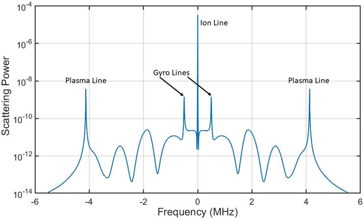
Figure 1. Theoretical calculation of Thomson scattering spectra (Froula et al., 2011), with sharp spectral features labeled. Plasma parameters for this plot are
The primary goal of this study is to calculate the plasma parameters required to observe an ion or gyro line feature in Thomson scatter spectra. This is the main scientific result of this study, and readers primarily interested in this result can skip to Section 4. However, this study is also intended to provide a complete and self-contained interpretation of Thomson scatter spectra. To do this, Section 2 reviews some standard results from kinetic plasma theory and then examines the dielectric function of Langmuir waves as a simple case. In Section 3, a physical justification for finding the minima of a dielectric function is developed by analogy with a driven oscillator. For a driven oscillator, the amplitude of oscillation is infinite when driven at the resonant frequency of a normal mode. Therefore, minima in the dielectric function correspond to the largest amplitude waves possible in a given frequency range, resulting in the ion and gyro line spectral features. Finally, Section 5 provides a classification of different types of scattering, including scatter off non-resonant modes, true incoherent scatter, and colloquial incoherent (actually coherent) scatter, while trying to clarify this obviously confusing terminology.
2 Roots of the dielectric function
In this section, we review the physical concept of a normal mode (Section 2.1) and how it applies to resonant waves in a plasma (Section 2.2). The Langmuir mode is a standard plasma wave, and Section 2.3 shows how the plasma line arises from standard root solves (normal modes) of the dielectric function.
2.1 Normal mode analysis
Normal mode analysis is a technique that finds the resonant frequencies of any oscillating system. Before using this technique to describe waves in a plasma, it is useful to consider a simple example of two masses with springs on each side, as shown in Figure 2. The equations of motion for the position of each mass are found by applying Newton’s second law,
where
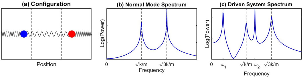
Figure 2. (a) Configuration of double spring system. Fourier transform of the masses’ positions (b) shows two distinct spectral peaks at the normal mode frequencies, marked by dashed vertical lines. In Section 3.2, a sinusoidal driving term is added to the equations of motion. (c) New spectral peaks that occur at driving frequencies ω1 and ω2.
This set of differential equations can be written in matrix form as
To find the normal modes of this system, Equation 3 is Fourier transformed, so effectively
In this form, the goal of normal mode analysis becomes apparent: create and solve an eigenvalue equation. The left-hand side shows the eigenvalues
The solution of Equation 5 is only possible if either
The two positive roots of
2.2 Deriving the dielectric function
The goal of normal mode analysis in a plasma is the same as the simple example above: to create an eigenvalue equation from a system of differential equations, then solve for the resonant frequencies of the plasma. The motions of a plasma are described at the kinetic level by the Vlasov equation for each species s:
The Vlasov equation is effectively a total time derivative of the distribution function, with the Lorentz force as the acceleration. To close this set of equations, the electric and magnetic fields need to be specified. While the following solutions and ideas work for general electromagnetic waves, we will restrict the analysis in this paper to electrostatic solutions since those are the wave modes measured by Thomson scatter radars. Therefore, Gauss’ law is appropriate to close the system. Additionally, we do not include a collision operator on the right-hand side of Equation 7 as collisions act to damp waves, but they do not significantly affect the resonant frequencies.
As defined in Equation 7, the Vlasov equation is nonlinear since the Lorentz force multiplies the velocity derivative of the distribution. For normal mode analysis to apply, the Vlasov equation and Gauss’ law need to be linearized and then Fourier–Laplace transformed. This is done using standard techniques, with each variable being decomposed as a zero-th order term and a first-order perturbation, such as
where k is the wavenumber from the spatial Fourier transform and
where
The Thomson scattering spectra is defined as
Taking Equation 10 for the densities of electrons and a single ion species, the electric field in Equation 9 becomes
the meaning of Equation 11 is clearer if the terms with
The initial value terms (
Physically, this shows the left-hand side as eigenvalues for the density perturbations on the right-hand side.
The integrals in Equation 13 are defined as the susceptibility of each species:
where
Solving for the perturbed electric field in Equation 15,
The dielectric function of a plasma is defined as
Equation 17 is the basis for the normal mode analysis of a plasma, and considerable literature exists on deriving equivalent forms (e.g., Bekefi, 1966). Solving Equation 17 means either
By writing Equations 16, 17 in terms of susceptibilities, the assumptions of electrostatic waves (
2.3 Example solution: the Langmuir mode
The simplest solution for a root of the dielectric function is the Langmuir mode. This wave mode is anticipated to occur at a frequency near the plasma frequency, and therefore ion dynamics can be neglected (Longley et al., 2021). Plasma lines are well known to be enhanced by photoelectrons (Longley et al., 2021), but for simplicity we will only analyze the case of thermally driven plasma lines such as those detected in Vierinen et al. (2017). Using the unmagnetized electron susceptibility, the dielectric function at high frequencies is (Supplementary Appendix A)
where the parameter
Figure 3 plots the real and imaginary parts of Equation 18 for different sets of plasma parameters. The resonant frequency is obtained by solving for the roots of
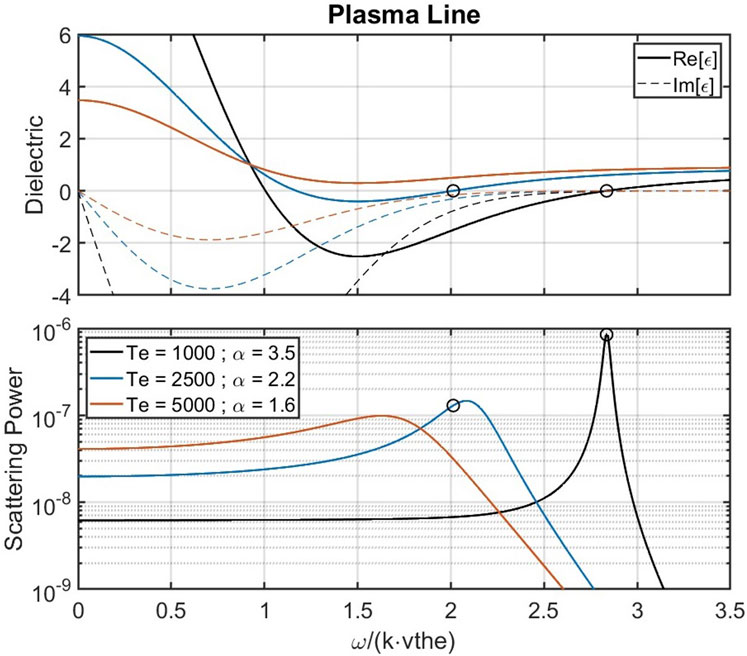
Figure 3. (Top panel) Real (solid curves) and imaginary (dashed curves) parts of the dielectric function near the plasma frequency. The low density (
Increasing the temperature once more to 5000 K in Figure 3 leads to
The transition of the plasma line/Langmuir mode from a normal to a quasinormal mode, and to what will later be defined as a non-resonant mode, appears to depend on the
The standard approximation is to anticipate
This creates the biquadratic equation in
For the Langmuir mode, it is easy to solve for a root of the dielectric function if the approximations of
The only free plasma parameter in Equation 23 is
For typical Thomson scatter experiments in the ionosphere,
The unmagnetized Langmuir mode and its relation to the plasma line are the easiest solutions to the dielectric function possible. Yet the solution still encounters several problems. The first is that if damping is present, we cannot solve for
3 Driven oscillations in a plasma
3.1 Initial value terms in the dielectric
In deriving the dielectric function in Section 2.2, the initial value terms from the Laplace transform in time were dropped so that a linear transformation of the electric field could be written and solved for eigenvalue frequencies. Keeping the initial value terms, the equation for the electric field becomes
Without the initial value terms on the right-hand side, this is Equation 17.
Equation 25 is no longer solvable for eigenvalues of the dielectric function. Mathematically, this is because the initial value term on the right-hand side means this is no longer a linear transformation of the electric field (failing the additive property
For normal modes of the system,
Taking a step back, the initial value terms of every particle are unknowable for a plasma experiment. Instead, an ensemble average is taken of Equation 25 to find the average electric field strength, weighted by the likelihood the plasma started in a particular initial state. The ensemble average is defined in Froula et al. (2011) as
where the zero-th order distribution
In squaring the left-hand side of Equation 28, there will be cross terms, but the standard treatment is to drop these by assuming that the initial positions of electrons and ions are uncorrelated (Froula et al., 2011). This assumption can be relaxed, though the resulting cross terms will only lead to an initial transient that decays as
where we define the source terms as
As an example, the Maxwellian distribution can be used for the initial distribution function
Comparing Equation 31 to Appendix Equation B3 shows the connection between the wave source terms S and the modified distributions M that describe Thomson scatter (Supplementary Appendix B). In general, these terms are proportional through the relation shown in Equation 32
Chapter 9 of Nicholson (1983) derives a similar expression to Equation 28 by neglecting ion dynamics and considering the electric potential of numerous moving test charges. Nicholson (1983) calls this result “fluctuations in equilibrium” but only applies the analysis to resonant Langmuir waves (i.e.,
3.2 Driven oscillations
Equation 29 is the desired result for interpreting the existence of density fluctuations in a plasma. The normal modes can still be obtained by setting the source terms S equal to 0 and solving for roots of
For physical intuition, we return to the mass-on-spring analogy of Section 2.1. The eigenvalue/eigenvector relation in Equation 5 can be written to include a sinusoidal driving force on each mass, giving the new relation
In this example, the frequency of the driving force
The source term in its simplest form (Equation 31) is the velocity distribution evaluated at the condition
Since
With this interpretation of the dielectric function, we are able to explain the concept of a non-resonant wave mode (e.g., Bekefi, 1966). Given a source term
For a source term that varies with frequency, the largest oscillations will occur at a balance between the minima of the dielectric function and the maxima of the driving source. This balance can lead to the strongest scatter occurring at frequencies shifted away from the resonant or non-resonant frequencies, as the next sections will demonstrate.
4 Minima of the dielectric function
In this section, the dielectric function is examined for minimum values that correspond to non-resonant versions of the ion-acoustic wave and the electrostatic whistler wave. In each case, these non-resonant waves are shown to correspond to distinct spectral features that are routinely observed in Thomson scatter experiments.
4.1 Ion line (ion acoustic mode)
For the ion-acoustic mode, both the electron and ion susceptibilities are important, and therefore the dielectric function is
With Equation 34, the dielectric function at low frequencies is then
The presence of the Dawson function requires a numerical solution to find any roots of Equation 35.
In the top panel of Figure 4, the real and imaginary parts of Equation 35 are plotted, showing that roots for
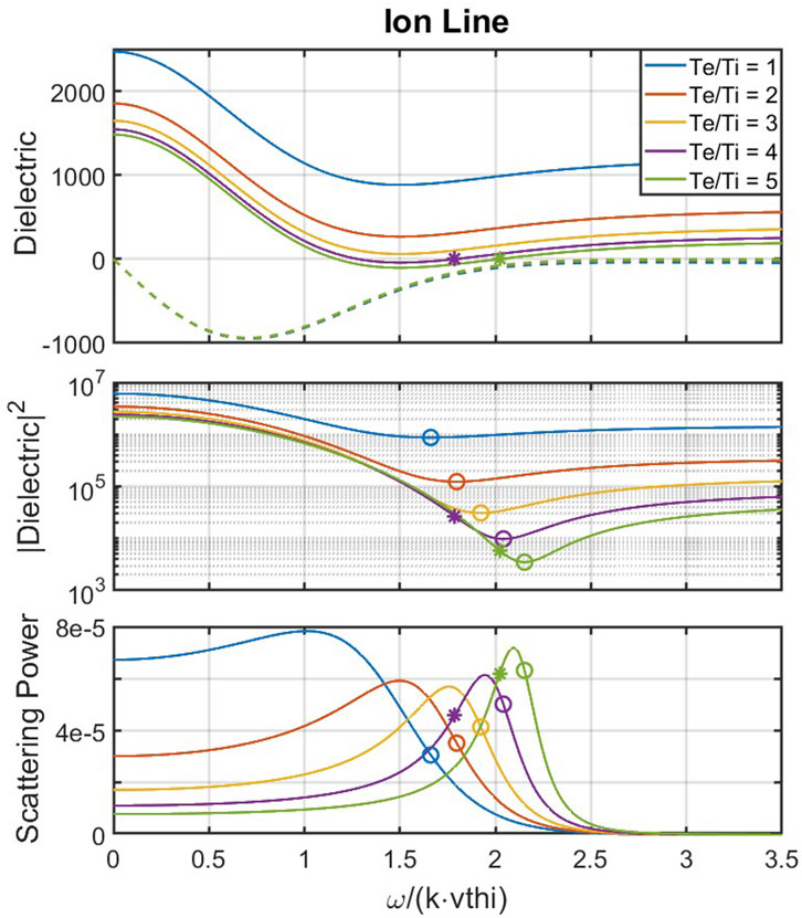
Figure 4. (Top panel) Real (solid curves) and imaginary (dashed curves) parts of the dielectric function near the ion-acoustic frequency for different temperature ratios. Stars mark location of roots to the real part of the dielectric, and those roots only exist if
Since
Typically,
The existence of an ion line in Thomson scatter experiments can be explained by the analogy with a driven oscillator described in Section 3.2. Waves will continuously be generated at low frequencies through Cherenkov radiation by particles moving at
The ion line is effectively unmagnetized for most aspect angles (Milla and Kudeki, 2011). Therefore, the driving source term for ion-acoustic waves is the Maxwellian distribution given by Equation 31. For electrons, the argument of the Maxwellian is
Despite the peak ion line power having no relation to the ion-acoustic frequency, we can still define the ion-acoustic frequency as either a root to
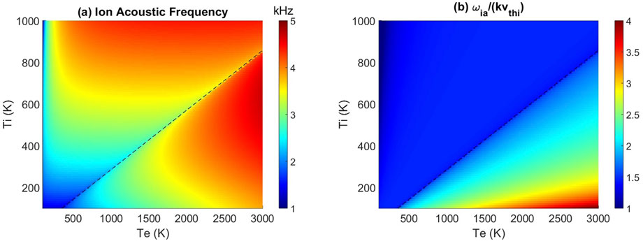
Figure 5. Solution for the ion-acoustic frequency (left). The dashed line is at
4.2 Gyro line (electrostatic whistler mode)
Gyro lines in Thomson scatter experiments are typically associated with the electrostatic whistler mode. The whistler mode is inherently magnetized and propagates via the electrons’ gyro motion around the magnetic field. The relatively low power of the gyro line compared to the plasma and ion lines has led to few observations of it—mostly by the Arecibo Observatory (Bhatt et al., 2006; Janches and Nicolls, 2007; Hysell et al., 2017) and the European Incoherent Scatter (EISCAT) radar (Malnes et al., 1993). The gyro line has remained an enigma within the ionospheric radar community due to its limited observations and the complicated magnetized terms in the dielectric function. Hysell et al. (2017) provides a thorough examination of the resulting whistler mode dispersion relation, concluding that a simple formula for the gyro line frequency does not exist.
The standard theory for the gyro line frequency
Using Appendix Equation A6 for the magnetized electron susceptibility and neglecting ions, the dielectric function is
With the harsh assumptions of Equation 39, roots to the real part of Equation 40 can be obtained through the following steps: 1) assuming that
From Equation 39 we have assumed
Note that in this study, the convention for the aspect angle is that
The assumptions in Equation 39 are required for a clean, simple solution for roots of the dielectric function. However, those assumptions are often not justified. At lower altitudes where gyro lines are often observed, both
where
The imaginary parts and therefore the damping of the whistler mode are dominated by the terms
As with the plasma line, the dielectric function at
The problem in solving either Equations 44 or 45, is that the Bessel and Dawson functions are transcendental, and a general solution is not tractable unless the assumptions of Equation 39 are made to justify Taylor expansions. It is therefore not possible to obtain an analytical solution for the gyro line frequency or conditions for its existence unless the approximations in Equation 39 are used.
The existing gyro line theory in Equations 41 and 42 relies on a narrow set of assumptions needed to simplify the magnetized dielectric function. The primary difficulty in a general solution is the presence of the infinite summation of the Bessel functions, the argument of which is called the “finite Larmor radius parameter” and is defined in Equation 46 as:
For infinitesimal b, only the
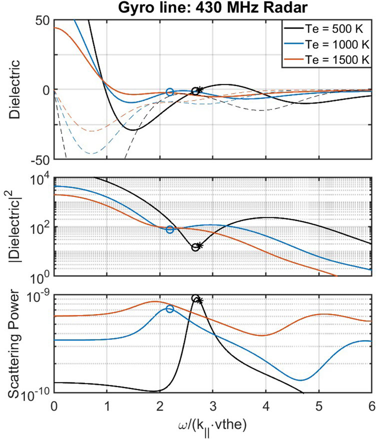
Figure 6. Similar to Figure 4 for the gyro line at Arecibo with
Figure 6 shows the gyro line’s dependence on electron temperature and therefore on b. At low temperature, the finite Larmor radius parameter is
The finite Larmor radius parameter can be minimized by either smaller temperatures, larger magnetic fields, or smaller wavenumbers. Note that changing the aspect angle will change b as well, but the tradeoff is that the argument
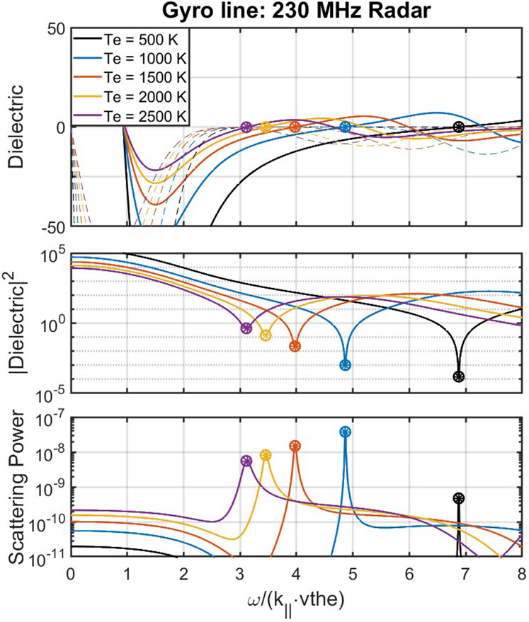
Figure 7. Similar to Figure 6, but for EISCAT 230 MHz parameters. Careful tracking of the imaginary part (dashed line, top panel) of the dielectric function shows that it is nearly 0 for each of the marked roots of
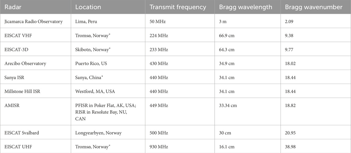
Table 1. Nominal parameters for selected Thomson scatter radars with routine ionosphere observations. Locations marked with an asterisk are the main transmit site of a multi-static system.
The dependence of the gyro line frequency on plasma parameters is investigated in Figure 8 for Arecibo and Figure 9 for EISCAT. In both figures, the aspect angle is fixed at 45°, with plots at different aspect angles shown in the supporting information. In panel (a) of each figure, the gyro line frequency is obtained by solving for the minima of
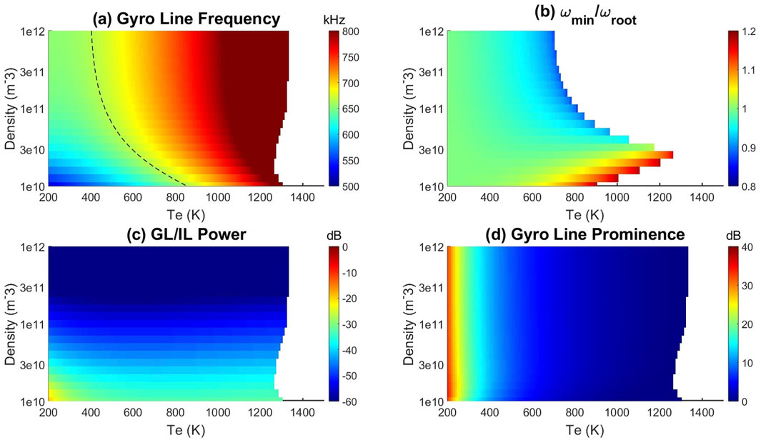
Figure 8. Gyro line for Arecibo (430 MHz) at a 45° aspect angle. (a) How the frequency obtained from minima of
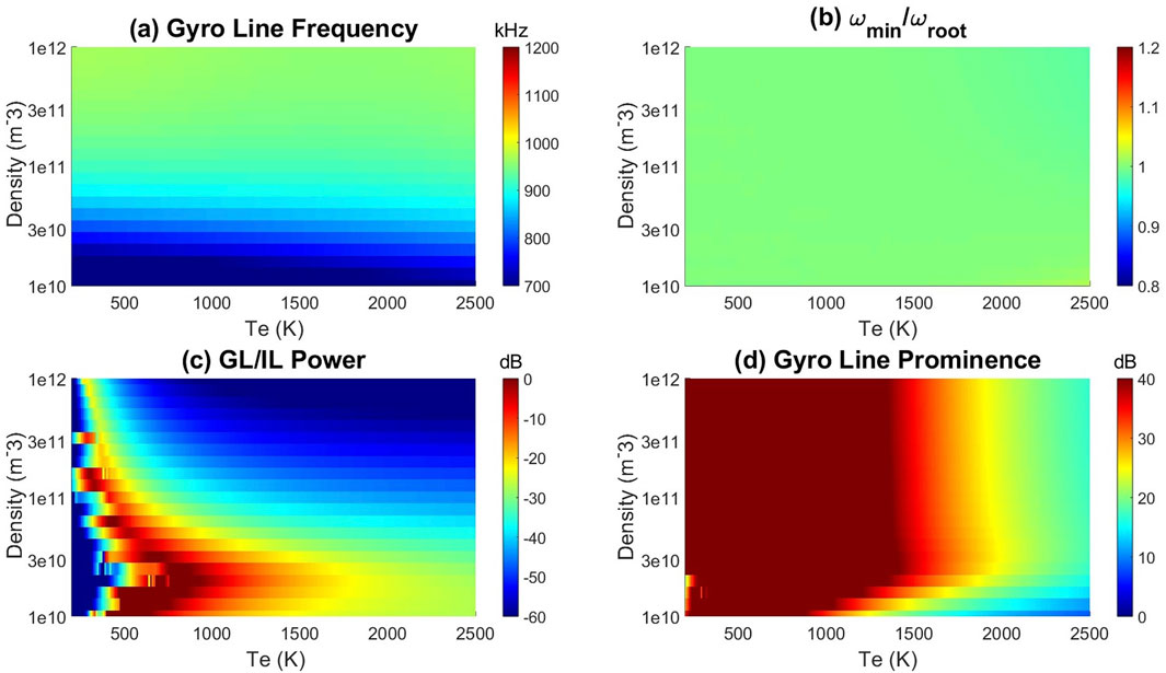
Figure 9. Same as Figure 8, but for EISCAT 230 MHz radar. At this radar frequency the gyro line frequency panel (a) has considerably less variation with density and temperature. Note in panel (b), both the minima finding technique and the root solve produce nearly identical answers at a wide range of temperatures. At low temperatures, the source term has a minimum near the gyro line frequency, leading to the absolute gyro line power (c) varying significantly with density and temperature despite the gyro lines being sharp and having the same relative prominence (d).
Since the gyro line is not influenced by ion dynamics, it is assumed that
The estimate in panel (c) shows how easily the gyro line could detect relative to the ion line. However, as the electron temperature increases, the gyro line experiences more Landau and cyclotron damping, broadening the spectral peak. Eventually, for high enough temperatures, the whistler mode becomes non-resonant and decreases in power while broadening substantially (Figure 6). This could lead to experimental difficulties in detecting the gyro line peak within a noisy measurement of the scattering spectra. Panel (d) in Figures 8, 9 estimates the relative prominence of the gyro line peak by calculating the power at
Solving for the gyro line frequency shows that the minima finding technique has two significant advantages over the typical root solving in normal mode analysis. First, the gyro line frequency can be calculated across a wider range of plasma parameters, better aligning with them where gyro lines are observed. Second, when a root does exist, it is significantly easier to find it with a bracketing method that searches for it near the non-resonant frequency. The root solving in this paper bracketed the root between
Figures 8, 9, along with the similar figures in the Supplementary Material, provide a full range of conditions needed for a radar to observe gyro lines at Arecibo and EISCAT VHF/3D. The data availability statement provides the code used to generate these figures and can readily create similar figures for different radars to predict the detectability of gyro lines.
4.3 What if there are no minima of the dielectric function?
Figure 6 plots the gyro lines at Arecibo for different electron temperatures. As the temperature rises, the root to the dielectric function disappears and then the minima of the dielectric disappear. Interestingly, a gyro-line-like feature remained present for each temperature. To examine this more closely, Figure 10 re-plots the same
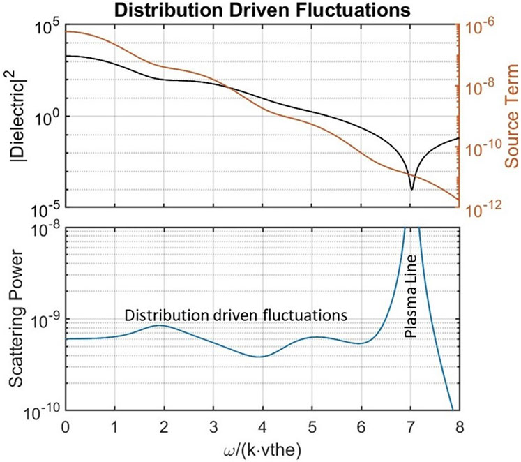
Figure 10.
In Figure 10, the only visible feature of the dielectric function at the vestigial gyro line is an inflection point. However, there is no obvious interpretation for what an inflection point in the dielectric function would physically mean, so we therefore attribute no significance to these inflection points. Furthermore, it has yet to be determined why there is scattering power at any of the other frequencies between the ion and plasma lines. Both the broad “vestigial gyro line” and the broader “shelf” feature between the ion and plasma lines can again be explained by the analogy of the driven oscillator. Previously, we focused on characterizing the plasma’s response to driven oscillations by looking for roots or minima of the dielectric function. The balancing part of this analogy is the source term that generates waves and drives fluctuations in the plasma. This source term is plotted in Figure 10. Again, there are inflection points at the peaks in the scattering power, but it does not appear to be fruitful or physically meaningful to try and characterize inflection points. However, it is clear that the non-constant source term balanced against the dielectric function leads to the bumps in the scattering spectra, as well as the general filling-in of the spectra.
The vestigial gyro lines and shelf features in Figures 3, 6, 7, and 10 are not dictated by the plasma’s response but by the driving of the system by the equilibrium distribution, and therefore we call these features “distribution driven fluctuations”. This choice of terminology reflects the dominant role of the source term in driving the fluctuations and creating a possibly measurable scattering power. For a distribution driven fluctuation to exist, the driving source term must be substantially large and continuously maintained in equilibrium in order to survive the ensemble average. In contrast, the normal modes in a plasma can be driven by an infinitesimal perturbation and still result in high scattering power.
4.4 Interpreting exotic spectra
The transition of gyro lines into broad distribution driven fluctuations is one example of non-standard Thomson scatter spectra. Other exotic spectra include perpendicular-to-B ion lines driven by Coulomb collisions (Kudeki and Milla, 2011; Milla and Kudeki, 2011), ion lines distorted by non-Maxwellian distribution functions (Goodwin et al., 2018), and plasma line splitting (Bhatt et al., 2008). In this section, we provide an example of interpreting these types of exotic spectra by examining the roots and minima of the dielectric function for plasma line splitting.
Plasma line splitting is a phenomenon first observed at Arecibo by Bhatt et al. (2008), where two distinct spectral peaks occur near the plasma frequency. This phenomenon was originally proposed in Salpeter (1961), predicting that two roots will appear in the dielectric function when the plasma frequency is near the second harmonic of the gyro frequency (
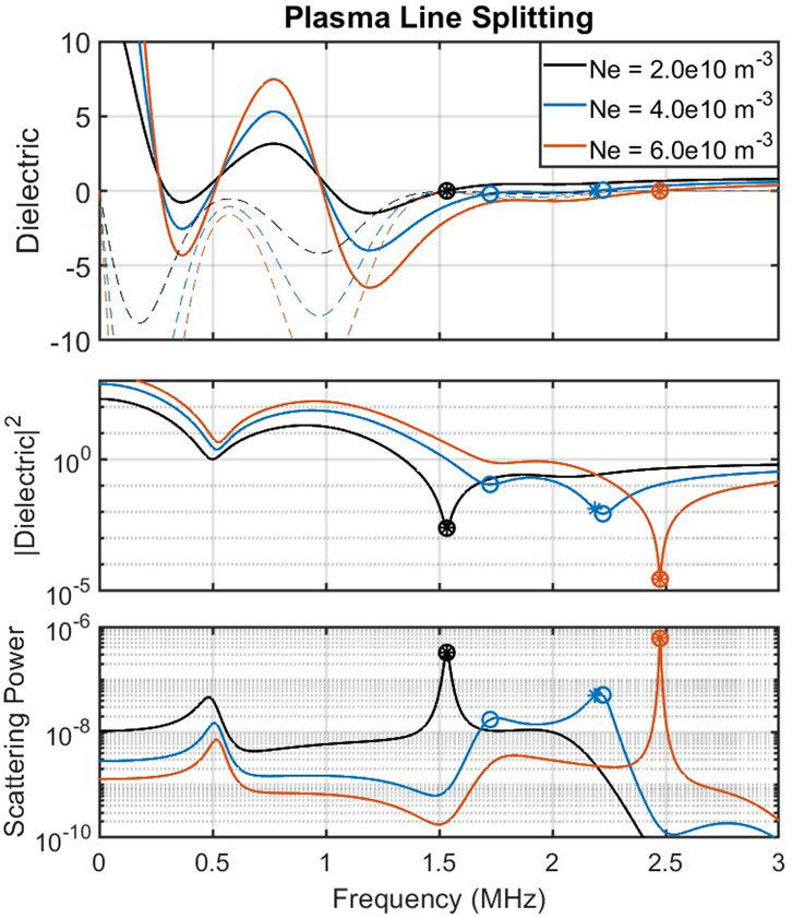
Figure 11. Dielectric function and scattering spectrum showing plasma line splitting. Note that x-axis is plotted in physical units of frequency.
The parameters in Figure 11 show the plasma line occurring at a lower frequency (∼1.5 MHz), then jumping to a higher frequency (∼2.5 MHz), with the plasma line splitting occurring as an intermediate step. To understand this transition further, Figure 12 plots the dielectric function for a narrower set of density values, with the inset showing where roots to

Figure 12. Zooming in on the dielectric function for split plasma lines. Densities correspond to
For each of the densities shown in Figure 12, the plasma line spectrum has two distinct peaks that sit on top of a broader spectral enhancement. This broader spectral enhancement is another example of distribution-driven fluctuations, where waves are continually excited near the second gyroharmonic. This is seen from evaluating the magnetized source term (Appendix Equation B4) with
5 Discussion
5.1 Types of Thomson scatter
This study has separately examined the dielectric function for the plasma line, the ion line, and the gyro line. These are common names for the spectral features observed in ionospheric Thomson scatter experiments, but as we have shown, the underlying wave mode or fluctuation may have a different physical origin depending on the plasma and radar parameters. Table 2 consolidates the terminology used to describe these different types of waves and fluctuations, the required conditions for that type of fluctuation to be present, and the corresponding spectral features. The usage of this terminology for Thomson scatter experiments is demonstrated in Figure 13, which revisits the sample Arecibo spectra plotted in Figure 1.
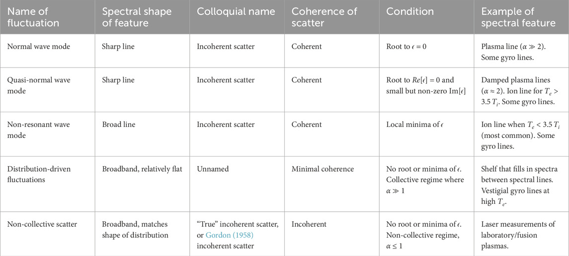
Table 2. Terminology of types of waves and fluctuations in a plasma.
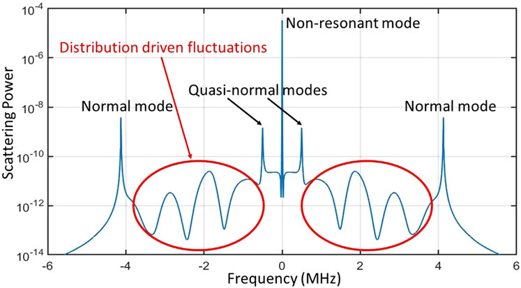
Figure 13. The same spectra from Figure 1 plotted again, with the spectral features labeled using terminology in Table 2. Note that distribution driven fluctuations have always been present in calculations of the full-bandwidth Thomson scatter spectra but have previously been ignored.
Table 2 also highlights a major problem within the ionospheric radar community: every measurement is erroneously called “incoherent scatter.” The original idea of ionospheric radar was posited in Gordon (1958) and assumed that electrons in the ionosphere would be randomly distributed, and therefore the phases of scattered waves would be random and the total backscatter would be incoherent. The terminology of “incoherent scatter” has persisted despite its well-known inaccuracy. Colloquially, an incoherent scatter radar is any ionospheric radar capable of making routine ion-line measurements with enough sensitivity to fit the ion line for plasma parameters. Formally, these are high-power and large-aperture Thomson scatter radars that operate in the collective scattering regime where
The distribution-driven fluctuations shown in Figure 10 are an interesting transition case between coherent and incoherent scatter. In terms of
5.2 Summary
The goal of this study has been to explain the presence of strong spectral features in Thomson scatter experiments when normal wave modes are not present. The ubiquitous measurements of ion lines in the ionosphere were a motivating puzzle which are now explained as non-resonant ion acoustic waves. Non-resonant waves are defined as frequencies where the magnitude of the dielectric function is at a local minimum. This holds a physical analogy to a driven oscillator, where waves are continuously created by Cherenkov radiation (source term) and the dielectric function characterizes the plasma’s response to continuously driven oscillations. Normal wave modes such as the Langmuir mode are also continuously driven, and their amplitudes are the result of a balance between the damping of the wave (dielectric function) and the driving source.
Our analysis used a specific framework (Froula et al., 2011) for calculating the dielectric function and source terms in a thermal plasma. This framework is ideal for this study as it is based on the plasma kinetic equations, but it suffers deficiencies in modeling collisions with the BGK operator. The more accurate Coulomb collision operators in Kudeki and Milla (2011) and Milla and Kudeki (2011) are required for accurate computations of the ion line at aspect angles within ∼10° of perpendicular to the magnetic field, and possibly the gyro line in the same regime. The ideas developed here can be generalized to this perpendicular-to-B regime by analyzing the dielectric functions from Kudeki and Milla (2011) and Milla and Kudeki (2011). For example, the ion line exactly perpendicular to B is created by collisional diffusion across magnetic field lines (Milla and Kudeki, 2011) and is best classified as a distribution driven fluctuation.
For extant radars, EISCAT-3D and EISCAT-VHF are best equipped to observe gyro lines and further explore the transition from normal modes at lower temperatures to quasi-normal or non-resonant wave modes at higher temperatures. Nonetheless, the highest resolution gyro line observations were made at Arecibo (Bhatt et al., 2006; Hysell et al., 2017). Future research will examine archived Arecibo experiments to look for gyro lines that transition from sharp spectral peaks to distribution driven fluctuations which would appear as a broad shelf feature between the ion and plasma lines. The −20 dB or lower power of the shelf feature places it at the edge of Arecibo’s sensitivity, although experiments such as Hagen and Behnke (1976) showed Arecibo to be capable of measuring spectra in the very weak, non-collective regime.
Data availability statement
The datasets presented in this study can be found in online repositories. The names of the repository/repositories and accession number(s) can be found at doi:10.5281/zenodo.15170116.
Author contributions
WL: Methodology, Writing – review and editing, Software, Conceptualization, Writing – original draft, Formal Analysis. LG: Conceptualization, Writing – review and editing, Funding acquisition, Writing – original draft, Formal Analysis. JV: Writing – review and editing, Formal Analysis, Conceptualization, Data curation.
Funding
The author(s) declare that financial support was received for the research and/or publication of this article. This work was supported by NSF awards AGS-2330254 and AGS-2431718.
Conflict of interest
The authors declare that the research was conducted in the absence of any commercial or financial relationships that could be construed as a potential conflict of interest.
The reviewer NI declared a past co-authorship with the author LG to the handling editor.
Generative AI statement
The author(s) declare that no Generative AI was used in the creation of this manuscript.
Any alternative text (alt text) provided alongside figures in this article has been generated by Frontiers with the support of artificial intelligence and reasonable efforts have been made to ensure accuracy, including review by the authors wherever possible. If you identify any issues, please contact us.
Publisher’s note
All claims expressed in this article are solely those of the authors and do not necessarily represent those of their affiliated organizations, or those of the publisher, the editors and the reviewers. Any product that may be evaluated in this article, or claim that may be made by its manufacturer, is not guaranteed or endorsed by the publisher.
Supplementary material
The Supplementary Material for this article can be found online at: https://www.frontiersin.org/articles/10.3389/fspas.2025.1607631/full#supplementary-material
References
Aponte, N., Sulzer, M. P., and González, S. A. (2001). Correction of the jicamarca electron-ion temperature ratio problem: verifying the effect of electron coulomb collisions on the incoherent scatter spectrum. J. Geophys. Res. 106 (A11), 24785–24793. doi:10.1029/2001JA000103
Beynon, W. J. G., and Williams, P. J. S. (1978). Incoherent scatter of radio waves from the ionosphere. Rep. Prog. Phys. 41 (6), 909–955. doi:10.1088/0034-4885/41/6/003
Bhatt, A. N., Gerken Kendall, E. A., Kelley, M. C., Sulzer, M. P., and Shume, E. B. (2006). Observations of strong gyro line spectra at arecibo near dawn. Geophys. Res. Lett. 33, L14105. doi:10.1029/2006GL026139
Bhatt, A. N., Nicolls, M. J., Sulzer, M. P., and Kelley, M. C. (2008). Observations of plasma line splitting in the ionospheric incoherent scatter spectrum. Phys. Rev. Lett. 100, 045005. doi:10.1103/PhysRevLett.100.045005
Bowles, K. L. (1958). Observation of vertical-incidence scatter from the ionosphere at 41 Mc/sec. Phys. Rev. Lett. 1, 454–455. doi:10.1103/PhysRevLett.1.454
Evans, J. V. (1969). Theory and practice of ionosphere study by thomson scatter radar. Proc. IEEE 57 (4), 496–530. doi:10.1109/proc.1969.7005
Froula, D. H., Glenzer, S. H., Luhmann, N. C., and Sheffield, J. (2011). Plasma scattering of electromagnetic radiation: theory and measurement techniques. Burlington, MA: Academic Press. doi:10.1016/B978-0-12-374877-5.00001-4
Goodwin, L. V., St.-Maurice, J.-P., Akbari, H., and Spiteri, R. J. (2018). Incoherent scatter spectra based on monte carlo simulations of ion velocity distributions under strong ion frictional heating. Radio Sci. 53, 269–287. doi:10.1002/2017RS006468
Gordon, W. E. (1958). Incoherent scattering of radio waves by free electrons with applications to space exploration by radar. Proc. IRE 46, 1824–1829. doi:10.1109/JRPROC.1958.286852
Hagen, J. B., and Behnke, R. A. (1976). Detection of the electron component of the spectrum in incoherent scatter of radio waves by the ionosphere. J. Geophys. Res. 81 (19), 3441–3443. doi:10.1029/JA081i019p03441
Hysell, D. L., Vierinen, J., and Sultzer, M. P. (2017). On the theory of the incoherent scatter gyrolines. Radio Sci. 52, 723–730. doi:10.1002/2017RS006283
Janches, D., and Nicolls, M. J. (2007). Diurnal variability of the gyro resonance line observed with the arecibo incoherent scatter radar at E- and F1-region altitudes. Geophys. Res. Lett. 34, L01103. doi:10.1029/2006GL028510
Kudeki, E., and Milla, M. (2011). Incoherent scatter spectral theories part I: a general framework and results for small magnetic aspect angles. IEEE Trans. Geosci. Remote Sens. 49 (1), 315–328. doi:10.1109/TGRS.2010.2057252
Longley, W. J. (2024). The generation of 150 km echoes through nonlinear wave mode coupling. Geophys. Res. Lett. 51, e2023GL107212. doi:10.1029/2023GL107212
Longley, W. J., Vierinen, J., Sulzer, M. P., Varney, R. H., Erickson, P. J., and Perillat, P. (2021). An explanation for arecibo plasma line power striations. J. Geophys. Res. Space Phys. 126, e2020JA028734. doi:10.1029/2020JA028734
Malnes, E., Bjørnå, N., and Hansen, T. L. (1993). European incoherent scatter VHF measurements of gyrolines. J. Geophys. Res. 98 (A12), 21563–21569. doi:10.1029/93JA02271
Milla, M., and Kudeki, E. (2011). Incoherent Scatter Spectral Theories—Part II: Modeling the Spectrum for Modes Propagating Perpendicular to B. IEEE Trans. Geosci. Remote Sens. 49 (1), 329–345. doi:10.1109/TGRS.2010.2057253
Salpeter, E. E. (1961). Plasma density fluctuations in a magnetic field. Phys. Rev. 122, 1663–1674. doi:10.1103/PhysRev.122.1663
Vallinkoski, M. (1988). Statistics of incoherent scatter multiparameter fits. J. Atmos. Terr. Phys. 50 (9), 839–851. doi:10.1016/0021-9169(88)90106-7
Vierinen, J., Gustavsson, B., Hysell, D. L., Sulzer, M. P., Perillat, P., and Kudeki, E. (2017). Radar observations of thermal plasma oscillations in the ionosphere. Geophys. Res. Lett. 44, 5301–5307. doi:10.1002/2017GL073141
Wikipedia (2023). “Quasinormal mode,” in Wikipedia, the free encyclopedia. Available online at: https://en.wikipedia.org/w/index.php?title=Quasinormal_mode&oldid=1149449449.
Keywords: Thomson scatter, ionosphere, radar, gyro line, wave generation, kinetic plasma, EISCAT
Citation: Longley WJ, Goodwin LV and Vierinen J (2025) The existence of non-resonant gyro lines and their detectability by Thomson scatter radars. Front. Astron. Space Sci. 12:1607631. doi: 10.3389/fspas.2025.1607631
Received: 07 April 2025; Accepted: 16 October 2025;
Published: 24 November 2025.
Edited by:
Farideh Honary, Lancaster University, United KingdomReviewed by:
Nickolay Ivchenko, Royal Institute of Technology, SwedenEliana Nossa, The Aerospace Corporation, United States
Copyright © 2025 Longley, Goodwin and Vierinen. This is an open-access article distributed under the terms of the Creative Commons Attribution License (CC BY). The use, distribution or reproduction in other forums is permitted, provided the original author(s) and the copyright owner(s) are credited and that the original publication in this journal is cited, in accordance with accepted academic practice. No use, distribution or reproduction is permitted which does not comply with these terms.
*Correspondence: William J. Longley, d2lsbGlhbS5sb25nbGV5QG5qaXQuZWR1