 Raman Mukundan1,2*
 Amy M. Keesee1,2
 José Paulo Marchezi1,2
 Victor A. Pinto3,4
 Michael Coughlan1,2
 Donald Hampton5
- 1University of New Hampshire, Department of Physics and Astronomy, Durham, NH, United States
- 2University of New Hampshire, Institute for the Study of Earth, Oceans, and Space, Durham, NH, United States
- 3Departamento de Física, Universidad de Santiago de Chile, Santiago, Chile
- 4Center for Interdisciplinary Research in Astrophysics and Space Sciences (CIRAS), Universidad de Santiago de Chile, Santiago, Chile
- 5Geophysical Institute, University of Alaska Fairbanks, Fairbanks, AK, United States
Geomagnetically induced currents (GICs) pose a significant space weather hazard, driven by geomagnetic field variation due to the coupling of the solar wind to the magnetosphere-ionosphere system. Extensive research has been dedicated to understanding ground-level geomagnetic field perturbations as a GIC proxy. Still, the non-uniform aspect of geomagnetic fluctuations make it difficult to fully characterize the ground-level magnetic field across large regions of the globe. Here, we focus on localized geomagnetic disturbances (LGMDs) in the North American region and specify the degree to which these disturbances are localized. Employing the electrodynamics-informed Spherical Elementary Current Systems (SECS) method, we spatially interpolate magnetic field perturbations between ground-based magnetometer stations. In this way, we represent the ground magnetic field as a series of heatmaps at high temporal and spatial resolution. We leverage heatmaps from storm time during solar cycle 24 to automatically identify LGMDs. We build a statistical picture of the frequency with which LGMDs occur, their scale sizes, and their latitude-longitude aspect ratios. Additionally, we use an information theory approach to quantify the dependence of these three attributes on the phase of the solar cycle. We find no clear influence of the solar cycle on any of the three attributes. We offer some avenues toward explaining why LGMDs might behave broadly the same whether they arise during solar maximum or solar minimum.
1 Introduction
Detailed descriptions of geomagnetic field activity near the surface of the Earth are of acute interest to a variety of communities. Utility providers (including, but not limited to, electric power transmission companies, railway companies, and fluid pipeline operators) can wield information about ground-level geomagnetic activity as a means to mitigate disruption to their infrastructure by geomagnetically induced currents (GICs) (Molinski, 2002; Patterson et al., 2023; Boteler and Trichtchenko, 2015). It is common to derive an induced geoelectric field, and the corresponding GICs, based on the measured geomagnetic field where no direct GIC measurements are available (Kelbert, 2020). Additionally, scientists value the ground-level magnetic field as an indicator for phenomena in the atmosphere, the inner magnetosphere, and beyond (e.g., Russell et al. (2008), Madelaire et al. (2023)). The United States government maintains a National Space Weather Strategy and Action Plan to safeguard economic interests and national security against the threat of geomagnetic storms among other space weather effects (National Science and Technology Council, 2019; National Science and Technology Council, 2023).
Of particular importance to these communities is knowledge about exactly where on Earth the horizontal component of the geomagnetic field,
Several explanations for the localization effect have been proposed. It is known that the nonuniform electric conductivity of Earth’s crust plays a role in determining the deflection of all components of the geomagnetic field, including
Some studies have investigated LGMD spatial scale by comparing readings at multiple stations, with attention paid to the geographic distance between those stations (Boteler and van Beek, 1999; Pulkkinen et al., 2015). To give some recent examples, Dimmock et al. (2020) found that the time derivative of the horizontal component of the magnetic field could be as much as three times higher at a single magnetometer station compared to the average of all magnetometers situated across a relatively small (
However, single-point measurements from magnetometers are insufficient to fully describe the size and shape of LGMDs because the distance between magnetometer stations may be larger than the scale sizes of the LGMDs themselves. That is to say, too sparse a distribution of magnetometer stations will not allow size scales to be precisely measured. There may be a few points of measurement, but the magnetic field’s behavior between those points is unknown. To overcome this deficiency, one requires a method by which to estimate
The goal of this investigation is to create a dataset of LGMDs on the North American region and to characterize their sizes and shapes during intervals of enhanced activity caused by geomagnetic storms. We use SECS to generate maps of geomagnetic field perturbations with high spatial resolution from a large cache of historical magnetometer data spanning storm times from 2009 through 2019. We then analyze the LGMDs that are displayed in these maps to reveal details about the frequency with which they occur, their spatial extent, and their longitude-latitude aspect ratios.
Finally, we quantify the solar cycle dependence of our LGMD dataset based on the Kullback-Leibler divergence, an important concept in information theory. Information theoretical approaches can be powerful tools when applied to space physics and space weather. Aryan et al. (2014) used the Kullback-Leibler divergence to quantify the relative importance of various solar wind parameters in the generation of chorus waves in the magnetosphere. Wing et al. (2018) studied the memory of the solar cycle and Snelling et al. (2020) studied the causal relationship between solar flares using transfer entropy and mutual information, respectively, two quantities which are closely related to the Kullback-Leibler divergence. Readers interested in further uses of information theory in space science should refer to Balasis et al. (2023), McGranaghan (2024), and references therein.
2 Data and data preparation
Obtaining the most complete picture of LGMD characteristics requires simultaneous data from multiple magnetometers. These data must describe long enough time scales so as to capture any variation due to the solar cycle. They must also exist at a fine enough temporal resolution to make clear how LGMD attributes evolve during periods of high geomagnetic activity. To address these requirements, we use 1-min cadence baseline-subtracted ground magnetic field data from the SuperMAG collaboration (Gjerloev, 2012). Our analysis in this work specifically examines the northward component of the perturbation vector of the interpolated magnetic field. We choose a single vector component because the northward (
This study examines LGMD scale size over a particular region of interest (though it could, in principle, be replicated to study LGMDs across any given section of Earth’s surface). We choose the region of interest to be within the quadrangle which is aligned with the standard geographic coordinate system, and which extends from 45
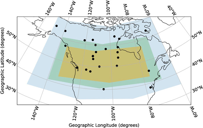
Figure 1. The magnetometers whose data are used to reconstruct LGMDs within mid-latitude North America. We only use magnetometers within the area indicated by the blue quadrangle. The green quadrangle shows the geographic extent of the Spherical Elementary Current System grid used to model magnetic perturbations, and the orange quadrangle represents the region over which our analysis is performed. Lines of geographic latitude and longitude are shown in light gray.
We use only data from magnetometers that are within the larger region extending from 35
We then discard timesteps wherein any magnetometer is missing a data point. Our SECS calculations described in Section 3 are only carried out when data from every magnetometer is available, which ensures consistency across timesteps with regard to SECS inversion. Therefore, we make this data availability restriction in order to preserve as many data points as possible while maximizing the number of magnetometers available for analysis.
Our choice of years across which our dataset spans – 2009 through 2019 – represents one full solar cycle (Solar Cycle 24). This allows all phases of the solar cycle to be captured, which is important because geomagnetic activity, as well as the magnetospheric processes that cause it, depend on the current solar cycle phase. We have chosen Solar Cycle 24 in particular because it is the most recent complete cycle and has the most SuperMAG stations with 1-min data available.
Finally, we examine only times during which geomagnetic storms occur. We use the same list of storms as Pinto et al. (2022), who define a storm as the period where the SYM-H index decreases below −50 nT and remains below this threshold for at least 2 h, plus 12 h of lead time before the SYM-H minimum and 24 h of recovery time afterward. Thus our final magnetometer dataset is composed of 183 storms and a total of 395,463 data points (equivalent to a total of 274.6 days). This is about 7% of the 5,784,480 data points that are in the full 2009–2019 period. We reduce our dataset in this way because we wish to study LGMDs during periods of enhanced geomagnetic activity.
3 Methods
3.1 Spherical elementary current systems
As mentioned before, extending
SECS interpolation operates by representing the ionospheric current distribution with a parametric model. Empirical determination of the model’s parameters at each moment in time is carried out based on magnetometer observations, which allows for the assumption that the model current distribution causes all observed ground-level geomagnetic activity. Once the model is fitted using this approach, one can apply the Biot-Savart law to the model current distribution in order to calculate the magnetic field deflection at any point within a region of interest.
The model current distribution is a superposition of curl-free and divergence-free vector functions defined on a common spherical surface, each with a different location for its pole. These basis functions are called elementary current systems. One is free to choose the placement of the poles of elementary current systems, but typically they are arranged in a latitude-longitude grid for convenience. By Helmholtz’s Theorem, any smooth, differentiable vector function can be exactly decomposed into such basis functions; using a finite number of basis functions at worst only approximates the original vector field. The divergence-free part (
One would typically consider the coordinate system in which
Here the currents are assumed to lie in an infinitely thin current shell of radius
Under the assumptions of this current-shell model, it can be shown that the ground magnetic effect of the curl-free current systems vanishes within the current surface (Fukushima, 1976). This allows
The constant
To determine the contributions from each current system, one can define a vector
Each element
When using Equation 2 to find the contribution of each current system to the magnetic field, it is important to notice again the difference between the geographic and the egocentric coordinate systems. These contributions are most easily added together when recognizing that a contribution vector
The total instantaneous magnetic field in the geographic coordinate system is then the sum of each contribution vector
3.2 Model details
We define our model current distribution as the superposition of a set of current systems whose poles are placed on a quadrangular latitude-longitude grid extending from 40.5
Poles are placed every 2°, making this a 10-by-35 array of current systems. The performance of SECS interpolation is not especially sensitive to small changes to the number and spacing of the current systems, so the 2-degree separation was chosen based on its use in McLay and Beggan (2010). We further validated this choice by performing joint Bayesian optimization of the number of rows and columns of current systems (while keeping the boundaries of the array fixed) using the Optuna package for Python (Akiba et al., 2019). The objective of this optimization was to minimize the absolute error between the model outputs at the location of each magnetometer and the measurements of the magnetometers themselves, averaged across magnetometers in each timestep, and then averaged across all timesteps in the dataset. The errors at each magnetometer were calculated using a leave-one-out scheme in which the model was fit using data from all magnetometers except the one in question, meaning a new model was fit for each magnetometer, all identical except for which magnetometer was omitted. The optimization found that the error was minimized for an 8-by-39 array of current systems. This agrees with our similar choice of array dimensions, whose error is less than 1% higher than the optimum. As such, we kept the 10-by-35 array so as to maintain a rounded 2-degree separation, as well as for possible future comparison to studies such as McLay and Beggan (2010).
Together with the number of rows and columns of current systems, the above procedure also jointly optimized a third quantity: the cutoff coefficient
When creating a SECS-based model, it is sometimes helpful to introduce an additional current sheet located at a negative altitude (that is, internal to the planet). Doing so may allow one to delineate which part of geomagnetic perturbations arise from ionosphere-associated phenomena and which perturbations arise from currents induced in the subsurface (Pulkkinen et al., 2003). However, the goal of the SECS model as it is used here is only to reproduce geomagnetic perturbations, not to explain them in terms of their contributing equivalent currents. As a result, the additional current sheet has not been employed in this study.
3.3 Identification and characterization of LGMDs
Measurements of
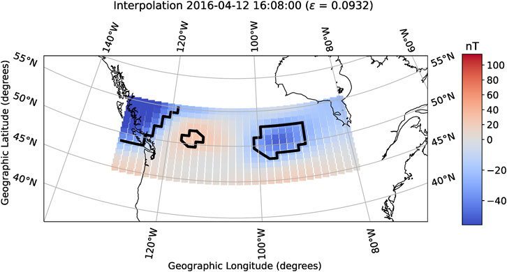
Figure 2. An example heatmap showing the result of interpolating
Once the heatmaps have been created, one can visually inspect them to view the estimated extent of LGMDs. However, we need to define a method to locate LGMD in a given heatmap. We do so here by granting a quantitative aspect to the definition of LGMD given in Section 1; that is, by defining a threshold value measure.find_contours function of the scikit-image Python package (Van Der Walt et al., 2014).
To identify LGMDs in this study, we define our perturbation threshold as
All our results in Section 4 are based on the heatmaps created using the procedure outlined in this section. Some are, more specifically, based on the perimeters of LGMDs identified in the heatmaps, each of which is calculated by adding up the distances between successive vertices of the contour that surrounds it. One must respect the spheroidal shape of Earth when computing these distances. Given two contour vertices with (latitude, longitude) coordinates (
In this work, we focus on perimeter as a measure of LGMD size. While there is no fundamental problem with investigating the behavior of LGMDs with different measures – for example, diameter – concentrating on the perimeter of LGMDs removes a degree of arbitrariness from the study. In the example of studying LGMD diameter, one would be forced to confront the question of along which direction to calculate that diameter, especially considering that LGMDs can vary widely in shape (an effect which is displayed in Figure 4). This is not an insurmountable issue; we hope that future work will extend the simpler baseline focus of this study to include other size metrics.
We also wish to study the shape of LGMDs, and pursue analysis of their aspect ratios as a way of doing so. We define the aspect ratio
with
4 Results and discussion
4.1 Full-solar-cycle distributions
After applying Spherical Elementary Current Systems and our contour-finding algorithm, we can study the behavior of LGMDs by examining relevant statistics of the resultant LGMD perimeter dataset. For that, we first consider the distribution of the number of LGMDs identified in each of our 395,463 heatmaps shown in Figure 3a. The distribution has a significant skew to the right, and no heatmap was ever observed to contain more than six LGMDs. A large proportion – about 58% – of heatmaps exhibit no LGMDs, though the exact amount is somewhat sensitive to the
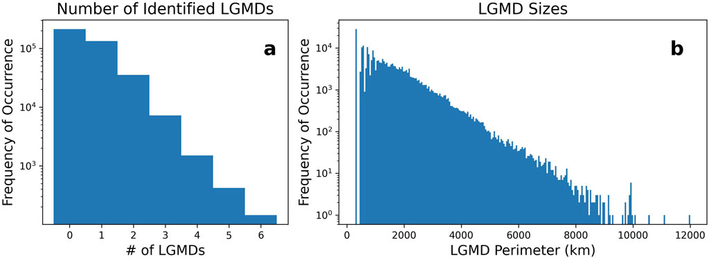
Figure 3. (a) The distribution of how frequently LGMDs are present in
We can also consider the perimeters of the LGMDs, as shown in Figure 3b. This figure describes the overall distribution of perimeter values. It is agnostic toward simultaneity and simply includes all LGMDs; that is, any two LGMDs contribute their perimeters toward this distribution even if they reside in the same heatmap. This distribution has a significant positive skew and shows that the mean, median, and mode LGMD perimeters are 1,620 km, 1,372 km, and 550 km respectively. Also of note is that the largest LGMD was observed to be 12,024 km in perimeter. As a point of comparison, the region of interest measures 9,344 km in perimeter, but it is possible for an LGMD perimeter to exceed this value if its associated contour forms a concave shape. However, most LGMDs are smaller than 9,000 km in perimeter, with only a handful of cases in the entire dataset close to the size of the region of interest.
Importantly, the typical perimeter of LGMDs as per these results is of the order that one would expect from estimates of the few-hundred-kilometer spatial scale derived using other methods, such as those mentioned in Section 1 (e.g., Dimmock et al. (2020); Dimitrakoudis et al. (2022)). This approximate correspondence between perimeter and diameter holds unless the LGMD in question is extremely oblong, which is quite rare according to the results contained in Figure 4.
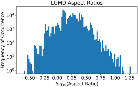
Figure 4. The distribution of the aspect ratios of all LGMDs over the entire solar cycle. Note that the distribution is centered on a positive number, meaning that LGMDs tend to be wider longitudinally than they are latitudinally.
Next, we examine the distribution of the aspect ratios of observed LGMDs. The distribution shown in Figure 4 is roughly symmetric about its central value at
One must note that our choice of the region of interest could be biasing this distribution in the positive direction by “cutting off” some data points on the negative end of the distribution. This is because the region of interest is wider in the longitudinal direction than it is in the latitudinal direction. To illustrate this, an LGMD which has been found to have a longitudinal extent of 1,400 km might be counted among those in Figure 4, but one with a latitudinal extent of 1,400 km would surpass the boundaries of the region of interest; its perimeter contours would not be closed, and thus it would not be represented in Figure 4. If this bias does exist, it could be corrected by extending the region of interest to have the same latitudinal extent as its longitudinal extent. However, for our purposes, this is not practical, because there are not sufficient magnetometers with available data to support such an expansion without reducing interpolation quality. Instead, we examined the distribution of aspect ratios of only LGMDs less than 1,000 km in perimeter. The LGMDs in this subset are too small to be cut off by the boundaries of the region of interest, even if they are oblong in the north-south direction. When normalized, the distribution of this subset is almost identical to the full distribution. We take this to be sufficient evidence that the dimensions of the chosen region of interest do not significantly impact the distribution of LGMD aspect ratios, at least for statistical purposes.
We have inspected the distributions of three attributes: the number of LGMDs per heatmap, the perimeter of LGMDs, and the aspect ratio of LGMDs. For readers interested in additional details concerning these LGMD attributes, plots of the distributions of perimeter and aspect ratio, separated by the number of simultaneous LGMDs, are available in the Supplementary Material. Additional statistics, whose significance is not analyzed in this work, are also available in the Supplementary Figure S3–S8.
4.2 Impact of solar cycle phase
We are also interested in whether the phase of the solar cycle has any relationship to the statistics explored in the previous sections. Therefore, we now proceed with an analysis of two different subsets of our dataset: the set of timesteps surrounding solar maximum (14 October 2012 through 31 January 2015) and those surrounding solar minimum (1 January 2009 through 31 October 2009 and 4 March 2018 through 31 December 2019) for Solar Cycle 24. The dates defining these intervals are set following Reyes et al. (2021), who precisely defined the phase boundaries for that solar cycle.
In this section, we reproduce each histogram from the previous section to include the solar maximum and solar minimum data subsets alongside the full dataset. These subsets each contain different numbers of data points because each represents a different range of instances in time. Therefore, the distributions shown have been normalized such that the area under each is 1. This is in contrast to the distributions in Section 4.1; those essentially represent the relevant attributes’ probability distributions, whereas the plots in this section show probability density functions (PDFs) because they have been normalized in this way. We show PDFs so that the data subsets may be directly compared. The distribution of the number of LGMDs per heatmap, though it represents a discrete variable as opposed to a continuous variable, can be represented by this normalization as a PDF because the “bin” width is 1.
The effects of separating solar minimum and solar maximum from the overall dataset are shown on the number of LGMDs (Figure 5), their perimeter (Figure 6), and their longitudinal-latitudinal aspect ratios (Figure 7). For each of these three statistics, the trends of the solar maximum and solar minimum subsets follow each other very closely. This motivates the question: are the differences that do exist between the subsets simply due to aleatoric variability (that is, do they only exist by chance?), or are they caused by some higher-order physical phenomena? To answer this question, we can compute a statistical divergence between the distributions corresponding to the solar maximum and solar minimum subsets. If this divergence is sufficiently large, that will be evidence against the hypothesis that the distributions differ only because of aleatoric effects.
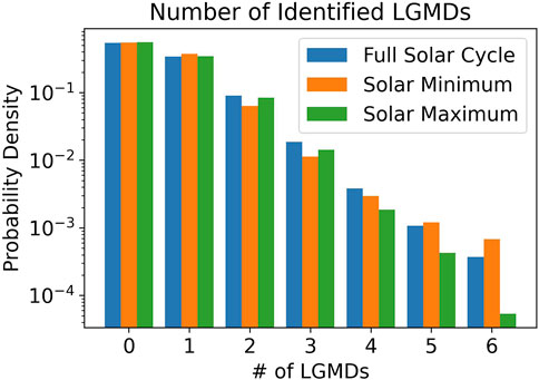
Figure 5. The blue bars represent the discrete probability density function (PDF) of the number of LGMDs per 1-min timestep over the entirety of Solar Cycle 24 and are equivalent to the histogram shown in Figure 3a. The orange and green bars show the same statistic for the solar minimum and solar maximum data subsets, respectively.
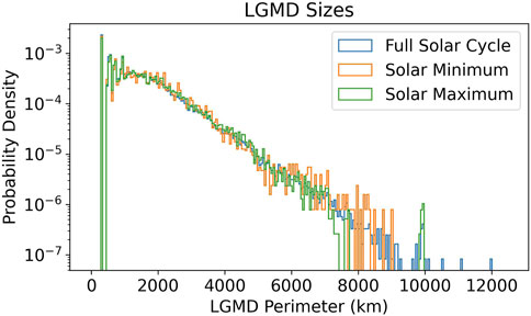
Figure 6. The blue trace represents the probability density function (PDF) of LGMD perimeter over the entirety of Solar Cycle 24 and is equivalent to the histogram shown in Figure 3b. The orange and green traces show the same statistic for the solar maximum and solar minimum data subsets, respectively.
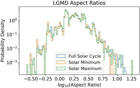
Figure 7. The blue trace represents the probability density function (PDF) of LGMD aspect ratio over the entirety of Solar Cycle 24 and is equivalent to the histogram shown in Figure 4. The orange and green traces show the same statistic for the solar minimum and solar maximum data subsets, respectively.
We first quantify the distance between a PDF associated with the solar maximum dataset,
Here, the sums are over the “bins” of the discretized PDFs. The width of each bin is
From an information theory perspective,
For this comparison, we simply define
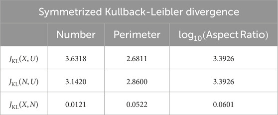
Table 1. Values for the symmetrized Kullback-Leibler divergence between various probability density functions (PDFs) formed from data from solar maximum (
It is clear from the reported values that the PDFs of each statistic shows much less divergence between solar maximum and solar minimum than they do between a uniform PDF and either solar maximum and solar minimum. The values of
The information theory perspective makes the
The total variation is computed outside of “logarithm space”, which avoids both drawbacks mentioned regarding
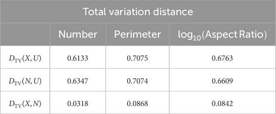
Table 2. Values for the total variation distance between various probability distributions formed from data from solar maximum (
One might expect the solar cycle to have an effect on the PDFs of these three LGMD attributes. After all, the solar cycle has an effect on the general geoeffectiveness of the solar wind–strong geomagnetic storms, storms due to coronal mass ejections, and strong ground-level geomagnetic activity are all more common during solar maximum, for instance (Webb, 1991; Richardson and Cane, 2012; Borovsky and Denton, 2006). However, as we move away from global size scales toward the smaller scales of LGMDs, we can not reject the hypothesis that the solar maximum and solar minimum distributions differ only because of aleatoric effects.
This does not necessarily mean that the solar cycle has no influence on the properties of LGMDs, only that any influence that does exist could not be detected with the methods used here. This is perhaps due to the fairly strict choice of the uniform distribution’s PDF as a benchmark PDF. One distribution being more similar to a uniform distribution than to the other solar cycle phase’s distribution – the criterion necessary to reject the baseline hypothesis – is a high bar to meet. There still may be some much smaller solar cycle effect that could require a more sensitive test to extract. We have used the uniform distribution’s PDF as a benchmark even still because other tests would include further amounts of arbitrariness. For instance, one could repeat this analysis on LGMD aspect ratio, replacing
Though this numerical analysis suggests that the distribution of aspect ratios does not strongly depend on the phase of the solar cycle, it does not reveal the physical processes that do determine the shape of the PDFs shown. This motivates a cause-and-effect analysis of LGMD aspect ratio, which likely deserves a study all to itself. Such a study could explore phenomena inside the magnetosphere, where the effect of the solar wind is modulated by a multitude of current systems, and it could connect these phenomena to the LGMD attributes lain out here. For instance, it could investigate the shape of localized structures embedded within the auroral electrojet and how they correspond to LGMDs. Similarly, heeding the results of Vandegriff et al. (2024) wherein points on Earth’s surface were magnetically mapped to spatially dispersed locations in the magnetotail, it may be of interest to examine the influence of large-scale features in the magnetosphere on LGMD aspect ratio.
Better establishing the empirical relationship between the solar wind, magnetospheric and ionospheric processes, and the characteristics of LGMDs will provide knowledge about the Sun-to-Earth phenomenological chain, and help to describe the link between LGMDs’ attributes and their drivers.
5 Conclusion
Understanding the complete spatial picture of ground-level geomagnetic disturbances is key when it comes to protecting GIC-susceptible infrastructure and developing our knowledge of magnetospheric physics. We use the Spherical Elementary Current Systems method to interpolate readings from 25 magnetometer stations in a way consistent with physics that drives activity in the magnetosphere. We densely sample the interpolations to create heatmaps showing the behavior of
From hundreds of thousands of these heatmaps, representing nearly all storm time in Solar Cycle 24, we analyze three statistics: the number of LGMDs per heatmap, the perimeters of LGMDs, and the aspect ratios of LGMDs. We develop frequency distributions of these statistics, finding that the typical scale size of LGMDs reconstructed via our methods agrees with scale sizes presented in related studies.
Finally, we subsample these frequency distributions to obtain ones that just represent data collected near solar maximum and ones that represent the same for solar minimum. For each statistic, the distributions from different phases of the solar cycle follow much the same trends; however, there are small differences between LGMDs that occur near solar maximum and ones that occur near solar minimum. These differences are determined to be insignificant by calculating the respective distributions’ probability density functions (PDFs), then comparing their Kullback-Leibler divergences and their total variation distances. In other words, the phase of the solar cycle does not strongly direct the attributes of LGMDs during storm time.
This study opens the path toward continued investigation of LGMDs and their drivers. Some possible areas of future study include investigating any correlation between LGMD attributes and the intensity of the storm during which those LGMDs occur. On the other hand, since we found no influence from the solar cycle, perhaps magnetospheric and ionospheric drivers are considerably more important than solar wind effects in determining the characteristics of LGMDs, and perhaps substorm activity in particular is more relevant than a focus on geomagnetic storms. This would agree with the findings of Ngwira et al. (2018), Ngwira et al. (2025) (among others), which emphasize the behavior of ionospheric currents and the mesoscale magnetospheric structures to which those currents systems are magnetically connected. It may, therefore, be constructive to correlate LGMD attributes with measurements of the ionosphere and aurorae above them, or, taking inspiration from Vandegriff et al. (2024), to correlate LGMD attributes with structures in the magnetotail in physics-based simulations.
Though we have investigated only the northward perturbation component
Similarly, our methods have applicability to the time derivative of magnetic field perturbations
There is no perfect interpolation method since all such methods are mere models of the physics governing the geomagnetic field. However, one cannot ignore the utility of interpolation in enabling advanced analysis techniques that could not be applied to single-point measurements. When its limitations are understood and accounted for, spatial interpolation has the power to facilitate geospace dynamics research and to enable the development of more effective and actionable predictive models.
Data availability statement
The magnetometer data which was used for this work is from the SuperMAG collaboration, and can be found at https://supermag.jhuapl.edu/. Software created for this work can be found in Mukundan (2025).
Author contributions
RM: Formal Analysis, Writing – review and editing, Methodology, Writing – original draft, Data curation, Investigation, Conceptualization. AK: Supervision, Investigation, Writing – review and editing, Funding acquisition. JM: Investigation, Writing – review and editing, Formal Analysis. VP: Investigation, Formal Analysis, Writing – review and editing. MC: Formal Analysis, Investigation, Writing – review and editing. DH: Writing – review and editing, Funding acquisition.
Funding
The author(s) declare that financial support was received for the research and/or publication of this article. This work was supported by NSF EPSCoR Award OIA-1920965 and NSF Award 2331527. VP thanks ANID grant SA772100112 and DICYT Regular grant 042431PA.
Acknowledgments
We thank all members of the MAGICIAN team at UNH and UAF who participated in the discussions leading to this article. We also thank the SuperMAG collaboration for providing the data used in this study.
Conflict of interest
The authors declare that the research was conducted in the absence of any commercial or financial relationships that could be construed as a potential conflict of interest.
Generative AI statement
The author(s) declare that no Generative AI was used in the creation of this manuscript.
Publisher’s note
All claims expressed in this article are solely those of the authors and do not necessarily represent those of their affiliated organizations, or those of the publisher, the editors and the reviewers. Any product that may be evaluated in this article, or claim that may be made by its manufacturer, is not guaranteed or endorsed by the publisher.
Supplementary material
The Supplementary Material for this article can be found online at: https://www.frontiersin.org/articles/10.3389/fspas.2025.1610276/full#supplementary-material
References
Akiba, T., Sano, S., Yanase, T., Ohta, T., and Koyama, M. (2019). “Optuna: a next-generation hyperparameter optimization framework,”. New York, NY, USA: Association for Computing Machinery, KDD ’, 2623–2631. doi:10.1145/3292500.3330701
Allen, J., Sauer, H., Frank, L., and Reiff, P. (1989). Effects of the march 1989 solar activity. Eos, Trans. Am. Geophys. Union 70, 1479–1488. doi:10.1029/89EO00409
Amm, O., and Viljanen, A. (1999). Ionospheric disturbance magnetic field continuation from the ground to the ionosphere using spherical elementary current systems. Earth, Planets Space 51, 431–440. doi:10.1186/BF03352247
Anderson, C. W., Lanzerotti, L. J., and MacLennan, C. G. (1974). Outage of the l4 system and the geomagnetic disturbances of 4 August 1972. Bell Syst. Tech. J. 53, 1817–1837. doi:10.1002/j.1538-7305.1974.tb02817.x
Aryan, H., Yearby, K., Balikhin, M., Agapitov, O., Krasnoselskikh, V., and Boynton, R. (2014). Statistical study of chorus wave distributions in the inner magnetosphere using Ae and solar wind parameters. J. Geophys. Res. Space Phys. 119, 6131–6144. doi:10.1002/2014JA019939
Balasis, G., Balikhin, M. A., Chapman, S. C., Consolini, G., Daglis, I. A., Donner, R. V., et al. (2023). Complex systems methods characterizing nonlinear processes in the near-earth electromagnetic environment: recent advances and open challenges. Space Sci. Rev. 219, 38. doi:10.1007/s11214-023-00979-7
Bolduc, L. (2002). GIC observations and studies in the hydro-québec power system. J. Atmos. Solar-Terrestrial Phys. 64, 1793–1802. doi:10.1016/S1364-6826(02)00128-1
Borovsky, J. E., and Denton, M. H. (2006). Differences between CME-Driven storms and CIR-Driven storms. J. Geophys. Res. Space Phys. 111. doi:10.1029/2005JA011447
Boteler, D. H., and Trichtchenko, L. (2015). “Telluric influence on pipelines,” in Oil and gas pipelines (John Wiley and Sons, Ltd), 275–288. doi:10.1002/9781119019213.ch21
Boteler, D. H., and van Beek, G. J. (1999)). August 4, 1972 revisited: a new look at the geomagnetic disturbance that caused the L4 cable system outage. Geophys. Res. Lett. 26, 577–580. doi:10.1029/1999GL900035
Campbell, K. M. (2017). A thesis submitted to the graduate faculty of the North Dakota state university of agriculture and applied science. Master’s thesis. Fargo, ND: North Dakota State University.
Cordell, D., Mann, I. R., Parry, H., Unsworth, M. J., Cui, R., Clark, C., et al. (2024). Modeling geomagnetically induced currents in the Alberta power network: Comparison and validation using hall probe measurements during a magnetic storm. Space weather. 22. doi:10.1029/2023SW003813
Dimitrakoudis, S., Milling, D. K., Kale, A., and Mann, I. R. (2022). Sensitivity of ground magnetometer array elements for GIC applications I: resolving spatial scales with the BEAR and CARISMA arrays. Space weather. 20, e2021SW002919. doi:10.1029/2021SW002919
Dimmock, A. P., Rosenqvist, L., Welling, D. T., Viljanen, A., Honkonen, I., Boynton, R. J., et al. (2020). On the regional variability of dB/dt and its significance to GIC. Space weather. 18, e2020SW002497. doi:10.1029/2020SW002497
Fukushima, N. (1976). Generalized theorem for no ground magnetic effect of vertical currents connected with pedersen currents in the uniform-conductivity ionosphere. Rep. Ionos. Space. Res. Jpn. 30, 35–40.
Gjerloev, J. W. (2012). The SuperMAG data processing technique. J. Geophys. Res. Space Phys. 117. doi:10.1029/2012JA017683
Heyns, M. J., Lotz, S. I., and Gaunt, C. T. (2021). Geomagnetic pulsations driving geomagnetically induced currents. Space weather. 19, e2020SW002557. doi:10.1029/2020SW002557
Kappenman, J. G. (2005). An overview of the impulsive geomagnetic field disturbances and power grid impacts associated with the violent sun-earth connection events of 29–31 October 2003 and a comparative evaluation with other contemporary storms. Space weather. 3. doi:10.1029/2004SW000128
Kelbert, A. (2020). The role of global/regional Earth conductivity models in natural geomagnetic hazard mitigation. Surv. Geophys. 41, 115–166. doi:10.1007/s10712-019-09579-z
Kelbert, A., Bedrosian, P. A., and Murphy, B. S. (2019). “The first 3D conductivity model of the contiguous United States,” in Geomagnetically induced currents from the sun to the power grid (American Geophysical Union AGU), 127–151. doi:10.1002/9781119434412.ch8
Kelbert, A., and Lucas, G. M. (2020). Modified GIC estimation using 3-D Earth conductivity. Space weather. 18, e2020SW002467. doi:10.1029/2020SW002467
Kullback, S., and Leibler, R. A. (1951). On information and sufficiency. Ann. Math. Statistics 22, 79–86. doi:10.1214/aoms/1177729694
Love, J. J., Lucas, G. M., Rigler, E. J., Murphy, B. S., Kelbert, A., and Bedrosian, P. A. (2022). Mapping a magnetic superstorm: march 1989 geoelectric hazards and impacts on United States power systems. Space weather. 20, e2021SW003030. doi:10.1029/2021SW003030
Madelaire, M., Laundal, K., Gjerloev, J., Hatch, S., Reistad, J., Vanhamäki, H., et al. (2023). Spatial resolution in inverse problems: the EZIE satellite mission. J. Geophys. Res. Space Phys. 128, e2023JA031394. doi:10.1029/2023JA031394
McGranaghan, R. M. (2024). Complexity heliophysics: a lived and living history of systems and complexity science in heliophysics. Space Sci. Rev. 220, 52. doi:10.1007/s11214-024-01081-2
McLay, S. A., and Beggan, C. D. (2010). Interpolation of externally-caused magnetic fields over large sparse arrays using spherical elementary current systems. Ann. Geophys. 28, 1795–1805. doi:10.5194/angeo-28-1795-2010
Molinski, T. S. (2002). Why utilities respect geomagnetically induced currents. J. Atmos. Solar-Terrestrial Phys. 64, 1765–1778. doi:10.1016/S1364-6826(02)00126-8
Mukundan, R. (2025). SEC-sizes: code for characterization of LGMD spatial scale. Release Publ. Front. Astronomy Space Sci. (1.2.1). doi:10.5281/zenodo.13227147
National Science and Technology Council (2023). Implementation plan of the national space weather strategy and action plan
Ngwira, C. M., Nishimura, Y., Weygand, J. M., Engebretson, M. J., Pulkkinnen, A., and Schuck, P. W. (2025). Observations of localized horizontal geomagnetic field variations associated with a magnetospheric fast flow burst during a magnetotail reconnection event detected by the THEMIS spacecraft. J. Geophys. Res. Space Phys. 130, e2024JA032651. doi:10.1029/2024JA032651
Ngwira, C. M., Pulkkinen, A. A., Bernabeu, E., Eichner, J., Viljanen, A., and Crowley, G. (2015). Characteristics of extreme geoelectric fields and their possible causes: localized peak enhancements. Geophys. Res. Lett. 42, 6916–6921. doi:10.1002/2015GL065061
Ngwira, C. M., Sibeck, D., Silveira, M. V. D., Georgiou, M., Weygand, J. M., Nishimura, Y., et al. (2018). A study of intense local dB/dt variations during two geomagnetic storms. Space weather. 16, 676–693. doi:10.1029/2018SW001911
Patterson, C. J., Wild, J. A., and Boteler, D. H. (2023). Modeling the impact of geomagnetically induced currents on electrified railway signaling systems in the United Kingdom. Space weather. 21. doi:10.1029/2022SW003385
Piccinelli, R., and Krausmann, E. (2014). Space weather and power grids – a vulnerability assessment. Joint Research Centre: Institute for Environment and Sustainability. doi:10.2788/20848
Pinto, V. A., Keesee, A. M., Coughlan, M., Mukundan, R., Johnson, J. W., Ngwira, C. M., et al. (2022). Revisiting the ground magnetic field perturbations challenge: a machine learning perspective. Front. Astronomy Space Sci. 9. doi:10.3389/fspas.2022.869740
Pirjola, R. (2000). Geomagnetically induced currents during magnetic storms. IEEE Trans. Plasma Sci. 28, 1867–1873. doi:10.1109/27.902215
Pulkkinen, A., Amm, O., and Viljanen, A.BEAR working group (2003). Separation of the geomagnetic variation field on the ground into external and internal parts using the spherical elementary current system method. Earth, Planets Space 55, 117–129. doi:10.1186/BF03351739
Pulkkinen, A., Bernabeu, E., Eichner, J., Viljanen, A., and Ngwira, C. (2015). Regional-scale high-latitude extreme geoelectric fields pertaining to geomagnetically induced currents. Earth, Planets Space 67, 93. doi:10.1186/s40623-015-0255-6
Reyes, P. I., Pinto, V. A., and Moya, P. S. (2021). Geomagnetic storm occurrence and their relation with solar cycle phases. Space weather. 19, e2021SW002766. doi:10.1029/2021SW002766
Richardson, I. G., and Cane, H. V. (2012). Solar wind drivers of geomagnetic storms during more than four solar cycles. J. Space Weather Space Clim. 2, A01. doi:10.1051/swsc/2012001
Rigler, E. J., Fiori, R. A. D., Pulkkinen, A. A., Wiltberger, M., and Balch, C. (2019). “Interpolating geomagnetic observations,” in Geomagnetically induced currents from the sun to the power grid (American Geophysical Union AGU), 15–41. doi:10.1002/9781119434412.ch2
Russell, C. T., Chi, P. J., Dearborn, D. J., Ge, Y. S., Kuo-Tiong, B., Means, J. D., et al. (2008). THEMIS ground-based magnetometers. Space Sci. Rev. 141, 389–412. doi:10.1007/s11214-008-9337-0
Schultz, A. (2009). EMScope: a Continental scale magnetotelluric observatory and data discovery resource. Data Sci. J. 8, IGY6–IGY20. doi:10.2481/dsj.SS_IGY-009
Snelling, J. M., Johnson, J. R., Willard, J., Nurhan, Y., Homan, J., and Wing, S. (2020). Information theoretical approach to understanding flare waiting times. Astrophysical J. 899, 148. doi:10.3847/1538-4357/aba7b9
Upendran, V., Tigas, P., Ferdousi, B., Bloch, T., Cheung, M. C. M., Ganju, S., et al. (2022). Global geomagnetic perturbation forecasting using deep learning. Space weather. 20, e2022SW003045. doi:10.1029/2022SW003045
Vandegriff, E. M., Welling, D. T., Mukhopadhyay, A., Dimmock, A. P., Morley, S. K., and Lopez, R. E. (2024). Exploring localized geomagnetic disturbances in global MHD: physics and numerics. Space weather. 22, e2023SW003799. doi:10.1029/2023SW003799
Van Der Walt, S., Schönberger, J. L., Nunez-Iglesias, J., Boulogne, F., Warner, J. D., Yager, N., et al. (2014). scikit-image: image processing in python. PeerJ 2, e453. doi:10.7717/peerj.453
Vanhamäki, H., and Juusola, L. (2020). “Introduction to spherical elementary current systems,” in Ionospheric multi-spacecraft analysis tools: approaches for deriving ionospheric parameters. Editors M. W. Dunlop, and H. Lühr (Cham: Springer International Publishing), 5–33. doi:10.1007/978-3-030-26732-2_2
Viljanen, A. (1998). Relation of geomagnetically induced currents and local geomagnetic variations. IEEE Trans. Power Deliv. 13, 1285–1290. doi:10.1109/61.714497
Viljanen, A., Nevanlinna, H., Pajunpää, K., and Pulkkinen, A. (2001). Time derivative of the horizontal geomagnetic field as an activity indicator. Ann. Geophys. 19, 1107–1118. doi:10.5194/angeo-19-1107-2001
Viljanen, A., and Tanskanen, E. (2011). Climatology of rapid geomagnetic variations at high latitudes over two solar cycles. Ann. Geophys. 29, 1783–1792. doi:10.5194/angeo-29-1783-2011
Webb, D. F. (1991). The solar cycle variation of the rates of CMEs and related activity. Adv. Space Res. 11, 37–40. doi:10.1016/0273-1177(91)90086-Y
Wei, L. H., Homeier, N., and Gannon, J. L. (2013). Surface electric fields for North America during historical geomagnetic storms. Space weather. 11, 451–462. doi:10.1002/swe.20073
Weygand, J. M., Amm, O., Viljanen, A., Angelopoulos, V., Murr, D., Engebretson, M. J., et al. (2011). Application and validation of the spherical elementary currents systems technique for deriving ionospheric equivalent currents with the north American and Greenland ground magnetometer arrays. J. Geophys. Res. Space Phys. 116. doi:10.1029/2010JA016177
Wik, M., Viljanen, A., Pirjola, R., Pulkkinen, A., Wintoft, P., and Lundstedt, H. (2008). Calculation of geomagnetically induced currents in the 400 kV power grid in southern Sweden. Space weather. 6. doi:10.1029/2007SW000343
Keywords: space weather, geomagnetically induced currents, localized geomagnetic disturbance, ground based magnetometer, spherical elementary current systems
Citation: Mukundan R, Keesee AM, Marchezi JP, Pinto VA, Coughlan M and Hampton D (2025) Localized geomagnetic disturbances: a statistical analysis of spatial scale. Front. Astron. Space Sci. 12:1610276. doi: 10.3389/fspas.2025.1610276
Received: 11 April 2025; Accepted: 21 July 2025;
Published: 13 August 2025.
Edited by:
Georgios Balasis, National Observatory of Athens, GreeceReviewed by:
Stavros Dimitrakoudis, National and Kapodistrian University of Athens, GreeceAdamantia Zoe Boutsi, National Observatory of Athens, Greece
Copyright © 2025 Mukundan, Keesee, Marchezi, Pinto, Coughlan and Hampton. This is an open-access article distributed under the terms of the Creative Commons Attribution License (CC BY). The use, distribution or reproduction in other forums is permitted, provided the original author(s) and the copyright owner(s) are credited and that the original publication in this journal is cited, in accordance with accepted academic practice. No use, distribution or reproduction is permitted which does not comply with these terms.
*Correspondence: Raman Mukundan, cmFtYW4ubXVrdW5kYW5AdW5oLmVkdQ==