Stacking data analysis method for Langmuir multi-probe payload

There are numerous small-scale electron density irregularities in the ionosphere. The coordination of multiple needle Langmuir probes (m-NLPs) enables in situ measurement of electron density with high spatial resolution. However, the theoretical analysis method based on orbital motion-limited (OML) theory cannot accurately estimate electron density, even at higher resolutions, due to limitations in satellite measurements. In addition, due to the influence of satellite charging and flight wake, the currents collected between multi-probes have low consistency, introducing significant error into the measurement results. This study uses a stacking algorithm to process m-NLP data and incorporates the International Reference Ionosphere (IRI) model to correct the predicted electron density (N_e) values. The integrated characteristics of the stacking model make full use of the advantages of various models such as multilayer perceptron (MLP), support vector regression (SVR), K-nearest neighbors (KNN), and light gradient boosting machine (LightGBM). The combination of integrated machine learning methods and IRI models greatly improves the accuracy of electron density measurements obtained by m-NLPs. The results indicate that even with poor consistency among the currents collected by multiple probes, the coefficient of determination (R²) of the prediction results using this method can reach 0.9553, which is 0.5079 higher than that of the traditional diagnostic method.

1 Introduction

There are some plasma clouds with different degrees of ionization in the ionosphere, which are called ionospheric irregularities (Aol et al., 2020; Reid, 1968). Their electron density (N_e) is higher or lower than the average ionization density of the surrounding environment. The spatial-scale distribution of irregularities ranges from meters to several thousand kilometers (Xing et al., 2018). The formation mechanisms and principles of irregularities at different scales are different, and their spatial and temporal evolution is also complex and dynamic. Numerous small-scale irregularities (ranging from meter to hectometer scale) that form at the edges of large- and medium-scale irregularities have been shown to cause severe amplitude and phase scintillation in radio waves. The rapid fading in short–medium waves and forward scattering of very high frequencies cause changes in signal trajectory and propagation delay in radio waves (Ning et al., 2012; Tereshchenko et al., 2006; Liu et al., 2021), leading to adverse effects on satellite communication and GNSS. Thus, it is important to measure the small-scale irregularities in the ionospheric plasma to mitigate their effects on radio wave communication.

Mott-Smith and Langmuir (1926) proposed a Langmuir probe diagnostic method to measure various plasma parameters. Later, this method has been widely used in space plasma exploration (Lebreton et al., 2006; Buchert et al., 2015; Wang et al., 2018; Lee et al., 2013). Traditional Langmuir probe systems rely on active voltage sweeping mechanisms (Lebreton et al., 2006; Fish et al., 2014) to acquire probe current measurements through which current–voltage (I–V) response profiles are derived. These data have been analyzed using theories such as orbital motion-limited (OML) theory (Mott-smith and Langmuir, 1926), the Allen–Boyd–Reynolds (ABR) theory (Allen et al., 1957), and the Bernstein–Rabinowitz–Laframboise (BRL) theory (Bernstein and Rabinowitz, 1959; Chen, 1965) to obtain plasma parameters such as N_e, temperature (T_e), and satellite floating potential (V_f) (Liu et al., 2023). The use of Langmuir probes in ionosphere satellites helped measure the distribution of ionospheric irregularities, enhancing our understanding of how ionospheric irregularities affect wireless communication and improving the reliability of modern communication systems.

The Langmuir probe can perform accurate in situ measurement of N_e in ionospheric plasma, which is one of the key parameters of the ionosphere composition and dynamics. The changes in N_e affect many aspects, such as radio communication, radar systems, satellite navigation, and space weather (Kintner and Ledvina, 2005; Chapin et al., 2006; Jakowski et al., 2001; Akala et al., 2012). These plasma irregularities exhibit dynamic spatial configurations that require quantification of N_e at meter to multi-kilometer scales for precise characterization of their spatiotemporal evolution (Kintner and Seyler, 1985). The limited correlation between the scanning frequency and plasma frequency of traditional Langmuir probes implies the difficulty in achieving high spatial resolution.

The new multi-needle Langmuir probe (m-NLP), conceived and engineered by Norway’s University of Oslo, was successfully deployed aboard the NorSat-1 during its orbital insertion from the Baikonur Cosmodrome, Kazakhstan, on 14 July 2017 (Hoang et al., 2018a). NorSat-1 completes dual equatorial traverses and polar transits within its 90-min orbital period. The m-NLP suite integrates a quad-probe configuration with independent bias-voltage control, featuring cylindrical sensors with 0.5 mm diameter and 25 mm axial dimensions. This payload achieves 1 kHz temporal resolution with 1 nA current measurement sensitivity (Hoang et al., 2018a), specifically designed to elucidate the formation mechanisms of small-scale plasma irregularities through high-precision N_e gradient measurements.

Jacobsen et al. (2010) proposed a new approach for the fast computation of N_e, which was later used to process m-NLP data. This method uses multiple fixed-bias Langmuir probes to simultaneously sample the plasma at different biases in the electron saturation region of the I–V characteristic. This method does not need scanning bias voltage or T_e at the beginning. The time required to obtain plasma parameters is short, which can greatly improve the spatial resolution of measuring N_e. Hereafter, the N_e calculation method proposed by Jacobsen et al. (2010) using linear fitting will be referred to as the traditional diagnostic method (TDM). Regarding the OML theory, the probe saturation current (I_p) and the applied bias voltage need to satisfy Equation 1 (Allen, 1992):

$I_p=eA{N}_e\sqrt{\frac{k_B{T}_e}{2\pi m_e}}\frac{2}{\sqrt{\pi }}{\left(1+\frac{eV}{k_B{T}_e}\right)}^{\beta },(1)$

where e is the electron charge, A is the surface area of the probe, k_B is the Boltzmann constant, m_e is the electron mass, and V is the bias voltage applied by the probe relative to the plasma space potential. In OML theory, the exponential β-value of the cylindrical Langmuir probe is 0.5, which is also used by m-NLP to calculate N_e. However, in practical situations, it is difficult to meet all the prerequisites of OML theory (Ma et al., 2019). For example, the plasma needs to satisfy the conditions such as (1) being collisionless, (2) following a non-drifting Maxwell distribution, (3) being non-magnetized, and (4) having an ion-collected current much smaller than the electron-collected current. It is reasonable to assume that the plasma in the ionosphere satisfies the above conditions. However, the limitations of the probe need to be discussed separately. At first, the potential carried on the probe must satisfy the following condition: (5) eV/kT > 0 or eV/kT ≥ 2 for cylindrical objects. The two requirements for the size of the probe are as follows: (6) the probe must be very thin, meaning that the probe radius r needs to be much smaller than the Debye length (λ_De), and (7) for a cylindrical probe, the probe length l needs to be much greater than λ_De.

The Langmuir probe payload working in space may not always meet the abovementioned seven conditions, especially (5) and (7). The TDM algorithm based on OML theory assumes a linear relationship between the square of the current collected and the voltage applied by the probe, which forms the basis for excluding T_e in calculating N_e. However, this only applies when the bias voltage applied to the probe is higher than the plasma potential, that is, the probe is in the saturation region of the I–V characteristics. However, the potential on the lower-potential probe of the CubeSat spacecraft is usually lower than the plasma potential due to the negative potential carried by the spacecraft (Ma et al., 2019). This prevents the probe from meeting the condition eV/kT ≥ 2, resulting in poor consistency in current collection between several probes and causing significant errors in the TDM results.

In addition, OML has certain requirements for the probe shape such that the probe radius should be smaller than the plasma λ_De, while the probe length far exceeds λ_De (Ma et al., 2019; Hoskinson and Hershkowitz, 2006). However, probes cannot satisfy this condition in the ionosphere, and in real practice, the probe length is usually similar to or even smaller than λ_De (Guthrie et al., 2021; Hoang et al., 2019). For example, the probe length of m-NLP is 25 mm, which, in most cases, is much smaller than the λ_De of the ionospheric plasma (ranges from 7 mm to 400 mm). Therefore, taking β directly as 0.5 is inaccurate. Many studies have shown that the value of β varies within a certain range (Jacobsen et al., 2010; Friedrich et al., 2013; Bekkeng et al., 2019; Hoang et al., 2018b). Certain studies also indicate that OML theory cannot be fully satisfied even with a probe length of 50 mm (Hoskinson and Hershkowitz, 2006). However, TDM did not account for errors in the N_e results caused by β deviations from 0.5.

The operational attitude of the spacecraft and contamination of probe surfaces can also lead to significant errors. When a spacecraft flies in low Earth orbit, one or more probes are likely to work within the plasma wake generated by the spacecraft’s movement. Under this orbital dynamics, the thermal motion of ions remains low relative to the platform velocity, while the thermal motion of electrons far exceeds the orbital velocity threshold. However, electrons can only penetrate the ion-rarefied wake region behind the probe within the range allowed by bipolar diffusion (Barjatya et al., 2009). Therefore, the operation of the spacecraft affects the collected current of the Langmuir probe in the ion and electron saturation regions, thus affecting N_e measurements (Ivarsen et al., 2019). Moreover, the surface of Langmuir probes is prone to adsorb water and neutral gas molecules, resulting in a weakened ability to absorb electrons or ions. The different levels of contamination between multiple probes can also cause significant errors.

In summary, due to the lack of many restrictions for the establishment of OML, there is a significant error between N_e provided by m-NLP and the actual observation. Thus, a new method is needed to accurately process the data generated by m-NLP, and this study proposes a method that combines the stacking algorithm in machine learning with m-NLP to estimate ionospheric plasma parameters, which can accurately capture the rapid changes in plasma N_e.

Section 2 introduces the theory of N_e measurement; Section 3 introduces several machine learning methods integrated in this model and the evaluation methods for the final results; Section 4 introduces the specific experimental process and provides a detailed analysis of the experimental results; and Section 5 presents the conclusion.

2 Theory of electron density measurement

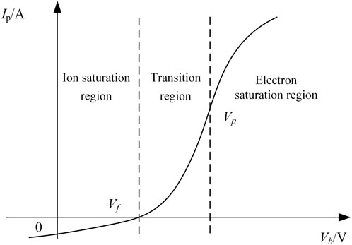
Figure 1 shows the representative I–V characteristics collected by the cylindrical Langmuir probe in plasma. The vertical axis shows the current collected by the probe (I_p), and the horizontal axis shows the scanning voltage (V_b) applied by the probe. The characteristic curve can be divided into three regions, namely, the ion saturation region, the transition region, and the electron saturation region, as the bias voltage changes from negative to positive. The voltage corresponding to the boundary point is the plasma floating potential (V_f) and plasma potential (V_p).

Figure 1

Figure 1. Representative I–V characteristic curves of the Langmuir probe.

Within the ion saturation region, V_b applied to the probe is much lower than V_p, causing it to repel most electrons, and only a very small number of high-energy electrons are captured by the probe’s sheath. Therefore, I_p can be considered to be mainly contributed by ions captured by the probe at this point while neglecting the role of a few electrons. Meanwhile, the negative potential of the probe attracts ions and forms an ion sheath around the probe. The condition of electrical neutrality is not met within the sheath (N_i > N_e), but outside the sheath, the plasma remains electrically neutral and is not disturbed by the probe’s potential. Ions enter the sheath at a random velocity, forming the ion saturation current (I_is) of the probe. The value of the ion saturation current is calculated as shown in Equation 2 for the Bohm current.

$I_{is}=-0.605e{N}_{i}A{\left(\frac{T_e}{m_i}\right)}^{\raisebox{1ex}{$1$}\!\left/ \!\raisebox{-1ex}{$2$}\right.},(2)$

where N_i is the ion density and m_i is the ion mass. Although I_is is theoretically constant, experimental observation shows that the ion saturation current does not remain fixed as V_b changes; instead, it gradually increases, especially for spherical and cylindrical probes. As V_b increases, the thickness of the sheath also changes, and the positive correlation with the absolute value of V_b results in an increase in the area for collecting ions, and consequently, the ion current does not saturate. Therefore, the ion saturation current cannot be described by the collection theory of planar probes, and at this point, Mott-Smith and Langmuir (1926) proposed OML theory.

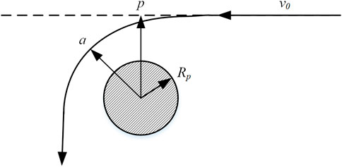
OML theory considers the motion path of individual ions at the microscopic level. It is assumed that a positive ion starts at infinity and moves at a velocity v₀ along a fixed direction toward a cylindrical Langmuir probe with a radius R_p, as shown in Figure 2. It is also assumed that the plasma potential at infinity is 0, and the probe potential is negative.

Figure 2

Figure 2. Trajectory of ions attracted by the probe.

In Figure 2, p is the distance between the incident orbit and the center point of the probe, and a is the distance from the center point of the probe after being attracted by the probe voltage and changing the orbit. According to the conservation of energy and angular momentum, if the distance between the ion and the center of the probe is less than R_p, the ion will be absorbed by the probe. Therefore, the ion flux (Φ_i) of the cylindrical probe with length L can be calculated using Equation 3:

${\mathrm{\Phi }}_i=2\pi R_{p}L{\left(1+\frac{V_a}{V_0}\right)}^{\raisebox{1ex}{$1$}\!\left/ \!\raisebox{-1ex}{$2$}\right.}{\mathrm{\Phi }}_r,(3)$

where V₀ is the voltage at the starting area of the ion, V_a is the voltage at the current area, and Φ_r is the random flux generated by the ion’s thermal velocity with the same Maxwell energy distribution (Equation 4).

${\mathrm{\Phi }}_r=N_i\sqrt{\frac{k_B{T}_i}{2\pi m_i},}(4)$

where T_i is the ion temperature. Integrating the distribution function of ions with Maxwell’s velocity distribution yields the total flux (Φ) of the probe, as shown in Equation 5:

$\mathrm{\Phi }=A{\mathrm{\Phi }}_r\left\{\frac{s}{a}\mathrm{erf}\left({\varphi }^{\raisebox{1ex}{$1$}\!\left/ \!\raisebox{-1ex}{$2$}\right.}\right)+e^x\left[1-\mathrm{erf}{\left(x+\varphi \right)}^{\raisebox{1ex}{$1$}\!\left/ \!\raisebox{-1ex}{$2$}\right.}\right]\right\},(5)$

where $x=-eV/k_B{T}_e$, $\varphi =a^{2}x/s^2-a^2$, and s is the thickness of the sheath layer.

When the three conditions s >> a, x >> ϕ, and T_i→0 are satisfied, Equation 5 can be approximated using Taylor expansion as

$I\underset{T_i\to 0}{⟶}ANe\frac{\sqrt{2}}{\pi }{\left(\frac{\left|eV\right|}{m_i}\right)}^{\raisebox{1ex}{$1$}\!\left/ \!\raisebox{-1ex}{$2$}\right.}.(6)$

Under orbital motion-limited theory, the relationship between ion saturation current and probe voltage for a cylindrical Langmuir probe can also be extended to calculate the electron saturation current, as shown in Equation 6.

The N_e rapid diagnostic method proposed by Jacobsen et al. (2010) only requires the use of two or more fixed-bias Langmuir probes. When the bias voltage is sufficiently positive, the electron current dominates, resulting in the probe being in the electron saturation current region. Squaring Equation 1 yields Equation 7:

${I_p}^2=\frac{2k_B{T}_e{e}^2{A}^2{N_e}^2}{{\pi }^2{m}_e}+\frac{2A^2{e}^{3}V{N_e}^2}{{\pi }^2{m}_e}.(7)$

V₁ and V₂ represent the two different biases of the probe, and I_p1 and I_p2 represent the currents collected by the two probes with different biases. The difference between the squares of two currents yields Equation 8:

${I_{p1}}^2-{I_{p2}}^2=\frac{2A^2{e}^3\left(V_1-V_2\right){N_e}^2}{{\pi }^2{m}_e}.(8)$

From Equation 8, N_e can be obtained as follows:

$N_e=\sqrt{\frac{{\pi }^2{m}_e}{2A^2{e}^3}\frac{\Delta \left({I_p}^2\right)}{\Delta V}.}(9)$

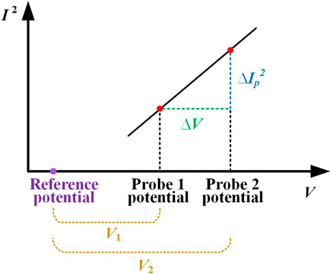
According to Equation 9, N_e can be calculated for two different biases through the probe and their corresponding collection currents. This suggests that, in the same plasma, the square of the probe collection current shows a linear relationship with the voltage difference, as shown in Figure 3.

Figure 3

Figure 3. Two fixed-bias probes used to diagnose electron density (N_e).

To make the results more reliable, bias voltages and corresponding currents are linearly fitted at no less than three points to solve N_e, which greatly improves the spatial resolution of plasma density.

3 Method of ensemble learning

Ensemble learning techniques have achieved state-of-the-art performance in diverse machine learning applications by combining the predictions from two or more base models (Mienye and Sun, 2022). In this study, multilayer perceptron (MLP), support vector regression (SVR), K-nearest neighbors (KNN), and light gradient boosting machine (LightGBM) were used as the base models.

3.1 Multilayer perceptron

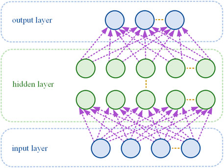
MLP is a widely used deep learning model, which is a feedforward network capable of solving linearly inseparable problems. Its structure is shown in Figure 4 (Kruse et al., 2022).

Figure 4

Figure 4. Multilayer perceptron structural model.

MLP consists of an input layer, several hidden layers, and an output layer containing multiple neurons in each layer. Each neuron receives and processes the output signals of all neurons in the previous layer and outputs them to the next layer. The calculations of each neuron in MLP are independent of each other. The input to a neuron is calculated as weighted sum of the outputs from the previous layer of neurons, added to a bias term. This calculation is shown in Equation 10:

$z_i^{\left(l\right)}={\sum }_{j=1}^{N^{\left(l-1\right)}}\left(w_{ij}^{\left(l\right)}·a_j^{\left(l-1\right)}\right)+b_i^{\left(l\right)},(10)$

where i represents the ith neuron, l represents the lth layer, N^(l-1) represents the number of neurons in the (L-1)th layer, w_ij^(l) represents the weight connecting the jth neuron in the (L-1)th layer to the ith neuron in the (L-1)th layer, a_j^(l-1) represents the output of the jth neuron in the (L-1)th layer, and b_i^(l) represents the bias of the ith neuron in the (l-1)th layer. Z_i ^(L) represents the input of the ith neuron in the lth layer.

Activation functions are used in each hidden layer and output layer of MLP to implement nonlinear transformations that enable the network to learn more complex representations and avoid network degradation. The common activation functions include the sigmoid function (Cox, 1958), ReLU function (Krizhevsky et al., 2017), tanh function (Lecun et al., 2002), and softmax function (Bridle, 1990). By inputting z_i^(l) into the activation function, the output a_i^(l) of the neuron can be obtained as shown in Equation 11:

$a_i^{\left(l\right)}=f\left(z_i^{\left(l\right)}\right).(11)$

3.2 Support vector regression

SVR is a regression application based on the support vector machine (SVM), which establishes the regression process by finding an optimal hyperplane that only considers the edge points around the training set (Smola and Schölkopf, 2004).

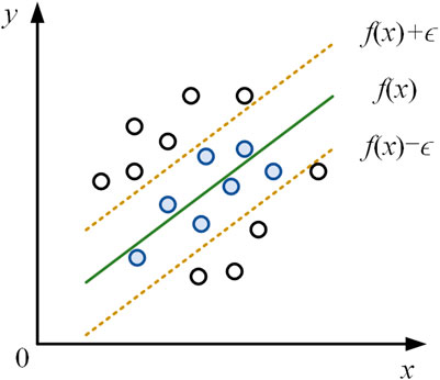
Assuming that the input feature x_i and the target output y_i form a pair of input–output data, f_(x) is the output function of this model. To avoid overfitting of the model and improve its generalization ability, a tolerance error ϵ is introduced so that the model does not need to fit all data points. The absolute value of the difference between f_(x) and y is acceptable within the tolerance error ϵ. When calculating the loss, only data points outside the tolerance error range are calculated. As shown in Figure 5, a spacing band is constructed with f_(x) as the center, with the upper boundary being f_(x)+ϵ and the lower boundary being f_(x)−ϵ. If |y_i − f_(xi)|≤ ϵ is satisfied, then the data point is within the interval band and the loss is 0.

Figure 5

Figure 5. Support vector regression schematic.

The kernel function maps the input features to a high-dimensional feature space and performs linear regression in the high-dimensional linear space to handle nonlinear problems. The commonly used kernel functions include linear kernel, polynomial kernel, Gaussian kernel, and Laplacian kernel.

3.3 K-nearest neighbors

KNN is an instance-based learning method that identifies K samples nearest to a given observation and uses their average to predict the target value. The calculation method of the average value (y’) is shown in Equation 12.

$y^{\prime }=\frac{1}{K}{\displaystyle \sum _{i=1}^K}{y}_i,(12)$

where K is the number of samples and y_i is the actual output value of the ith nearest neighbor sample of the predicted point. The core idea of KNN is to use information from surrounding neighbors for prediction. The choice of K value affects the model’s and the smoothness of its prediction. This indicates that a smaller K makes the model more sensitive, while a larger K results in smoother prediction results.

3.4 Light gradient boosting machine

LightGBM is based on a gradient boosting framework with the core ideas of the histogram algorithm, a leaf-wise growth strategy with depth limitation, unilateral gradient sampling, and mutually exclusive feature bundling (Ke et al., 2017).

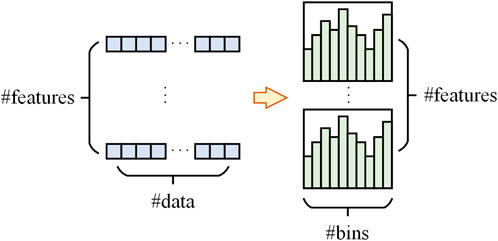
The histogram algorithm is an efficient decision tree learning algorithm that has a small memory footprint. Unlike traditional algorithms that sort feature values at each split point, the histogram algorithm divides continuous feature values into discrete intervals and finds the optimal split within those intervals. This approach reduces computational complexity while maintaining high accuracy, as shown in Figure 6.

Figure 6

Figure 6. Schematics of the histogram algorithm.

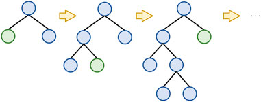
LightGBM uses the leaf-wise growth strategy, as shown in Figure 7. The leaf-wise growth strategy prioritizes splitting the leaf nodes with the highest gain, and the decision tree stops growing at a certain depth. This limits the complexity of the tree and prevents overfitting while ensuring a fast and efficient model speed.

Figure 7

Figure 7. Leaf-wise tree growth strategy.

3.5 Stacking theory

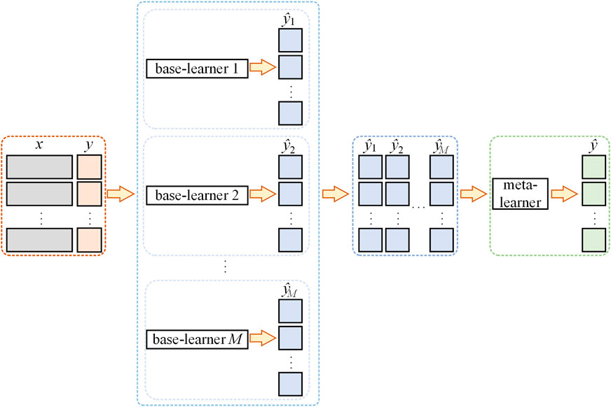
Ensemble learning combines multiple learners into a more powerful learner that can combine multiple models with reasonable strategies to achieve higher performance and generalization ability. The three main methods of ensemble learning are bagging, boosting, and stacking (Ribeiro and Dos santos coelho, 2020). As shown in Figure 8, two types of learners in the stacking model are base learners and meta-learners. The base learner is the underlying learner of the stacking model, which is the first-level learner that directly learns from the raw data and generates first-level prediction results. The meta-learner is the top-level learner of the stacking model and acts as a second-order learner, typically represented by a single model instance. The meta-learner integrates and modifies the output of the base-learner to reduce the bias and variance of the model. It can also generate the final prediction results and improve the stability and accuracy of the model.

Figure 8

Figure 8. Principles of the stacking model.

The stacking model takes the prediction results of multiple different base learners as input and trains a meta-learner. The learners in each layer can be different types of models, such as decision trees, linear models, and neural networks.

The ensemble feature of the stacking model enables the full utilization of the advantages of each base learner, compensates for the shortcomings of individual learners, and reduces the impact of overfitting of a model on specific data. Its advantage is the ability to extract diverse information from data and adapt to various types of data features and task objectives. This model has high diversity and generalization ability, and its architecture is also easy to expand. However, there is often a risk of overfitting in the stacking model when faced with limited input data, so some overfitting strategies must be used during the training process of the model. This study used k-fold cross-validation (k = 5) during both base-learner training and meta-learner stacking. For neural network-based base learners (MLP, etc.), we applied L2 regularization (λ = 0.01) and dropout (rate = 0.2) to reduce model complexity and avoid overfitting.

4 Experimental process and results

The data used in this study come from the m-NLP payload and the IRI 2016 model. The m-NLP provides probe current data required for prediction, while IRI 2016 provides N_e data corresponding to the probe’s data. The NorSat-1 m-NLP data can be downloaded from the data portal website of the University of Oslo (M-nlp, 2024). According to the location and time information provided by the m-NLP, the corresponding N_e data can be obtained from the IRI 2016 model (Bilitza et al., 2014).

IRI 2016 is an international ionospheric reference model developed jointly by the International Committee on Space Research (COSPAR) and the International Union of Radio Science (URSI) to describe the global distribution of key parameters such as N_e, N_i, and T_e in the Earth’s ionosphere (Bilitza et al., 2014). IRI 2016 provides standardized and empirical predictions of ionospheric parameters, and the output ionospheric plasma parameters depend on solar activity intensity and the geomagnetic index. Compared to real detection results, the displayed parameters are smoother. However, due to the lack of in situ exploration references in space, this study used the result output by IRI 2016 as reference values. Although there are errors compared with the real ionospheric environment, this study mainly aims to verify the effectiveness of machine learning methods in predicting N_e. IRI 2016 can provide corresponding ionospheric parameters by inputting information such as time and the satellite’s location.

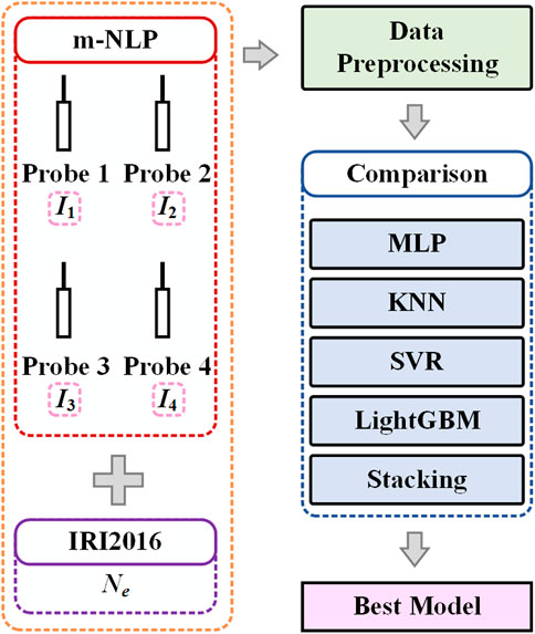
The experimental process is shown in Figure 9. As mentioned earlier, the probe data from the m-NLP and the N_e data from IRI 2016, required for this analysis, can be obtained from their respective websites and together constitute the original dataset. The raw data are then pre-processed, including steps such as filtering and normalization. Finally, we train the single model and the stacking model of various structures subsequently and use the evaluation indicator to compare the prediction effect of each model to determine the best model.

Figure 9

Figure 9. Method of machine learning for processing data from the multi-needle Langmuir probe.

The predictive effectiveness of this model during training can be quantified using evaluation indicators. The evaluation indicators can also identify problems in the model and determine whether overfitting and underfitting have occurred. This analysis chooses mean squared error (MSE) as the loss function given in Equation 13:

$\text{Loss}=\text{MSE}=\frac{1}{n}{\displaystyle \sum _{i=1}^n}{\left(y_i-{y_i}^{\prime }\right)}^2,(13)$

where y_{i is} the label value, y_i’ is the model’s prediction value, and n is the number of samples. The MSE intuitively measures the squared difference between the predicted and actual values, making the loss function easier to interpret.

The model’s predictive performance is measured using four indicators: mean absolute error (MAE), mean absolute percentage error (MAPE), root mean square error (RMSE), and coefficient of determination (R²).

The MAE can show the actual situation of prediction error and is given in Equation 14:

$\text{MAE}=\frac{1}{n}{\displaystyle \sum _{i=1}^n}\left|y_i-{y_i}^{\prime }\right|.(14)$

The MAE provides a quantitative measure to represent the average prediction error size of a model. It measures the average absolute difference between the predicted and true values. Unlike the MSE, the MAE does not assign excessive weight to large errors, suggesting that it is less sensitive to outliers.

The MAPE provides a simple and clear representation of the ratio between the prediction error and true value. The equation for MAPE is shown in Equation 15:

$\text{MAPE}=\frac{1}{n}{\displaystyle \sum _{i=1}^n}\left|\frac{y_i-{y_i}^{\prime }}{y_i}\right|.(15)$

The RMSE function reflects the average error value and can be calculated using Equation 16:

$\text{RMSE}=\sqrt{\frac{1}{n}{\displaystyle \sum _{i=1}^n}{\left(y_i-{y_i}^{\prime }\right)}^2.}(16)$

The RMSE has the same unit of measurement error as the raw data. This allows the performance of the model to be understood at the scale of actual observations without being affected by the absolute size of the data. The RMSE is more sensitive to large errors than the MAE, and if the model produces significant errors on some data points, the RMSE will be more pronounced.

R² can quantify the goodness of fit of a regression model with values spanning from 0 to 1. The closer R² is to 1, the better the model’s goodness of fit and its explanatory power for changes in the observed values. R² can be calculated as shown in Equation 17:

${\mathrm{R}}^2=1-\frac{{\displaystyle {\sum }_{i=1}^n}{\left(y_i-{y_i}^{\prime }\right)}^2}{{\displaystyle {\sum }_{i=1}^n}{\left(y_i-{\overline{y}}_i\right)}^2},(17)$

where ȳ_i represents the average of the actual values.

4.1 Data preprocessing

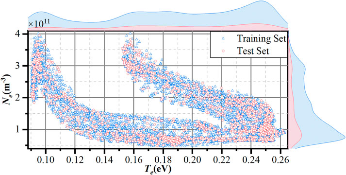
We used m-NLP to obtain probe and satellite orbit data for 5 days, 5 May, 7 May, 8 May, 2 August, and 3 August 2021, which were relatively complete and had high continuity. The longitude, latitude, altitude, and time in m-NLP data can be used to find the corresponding T_e and N_e data in IRI 2016. IRI 2016 and m-NLP data were filtered, and some data were removed as some periods of m-NLP data only contained orbital data and did not include probe data. After filtering, there are 1,420 sets of data per day, resulting in a total of 7,100 datasets over 5 days. We combined the four current values of the four probes with the N_e data from IRI 2016 to obtain the raw dataset and divided it into training and testing sets in a 4:1 ratio. The N_e and T_e distribution results of the data are shown in Figure 10. The distribution ranges of N_e and T_e are 4.65 × 10¹⁰ m^-3– 4.02 × 10¹¹ m^-3 and 0.09 eV–0.26 eV, respectively.

Figure 10

Figure 10. T_e and N_e distribution of the dataset.

The difference in the dimension of feature vectors can cause the objective function to shift, and normalization is also required between different evaluation indicators. The difference in dimensions can also cause the descent direction to deviate from the minimum value direction and generate violent fluctuations during model gradient descent, ultimately leading to excessively long training time and even ineffective training results. So, we standardize the data before inputting it into the model to eliminate the dimensional influence between various indicators. The zero mean normalization (Equation 18) is a method that can perform linear transformations on data. It can shift the mean of data to 0, help eliminate mean bias, and facilitate model learning of data features.

$x^{\prime }=\frac{x-\mu }{\sigma },(18)$

where μ is the average and σ is the standard deviation of the characteristic values. The zero mean normalization can eliminate mean bias between features by shifting the mean of the data to 0, and this helps the model better capture the relationships between features. The method reduces the bias during the model training process and can accelerate the convergence speed of the model. After standardization, the data present a uniform distribution relative to the center, and optimization algorithms can, thus, quickly find the optimal solution. The zero mean normalization does not change the scale of the data and hence does not affect the feature scale of the model. The standardized data have zero mean and unit variance, which makes the weights of features easier to interpret and reflects their relative contributions to the output.

4.2 Optimizer

The search for the optimal solution is a crucial objective in optimization problems. To achieve this goal, numerous optimization algorithms have been proposed, including the gray wolf optimizer (GWO) (Mirjalili et al., 2014), whale optimization algorithm (WOA) (Mirjalili and Lewis, 2016), and Bayesian optimization (BO) (Frazier and Bayesian optimization, 2018). GWO is a global optimization algorithm inspired by the hierarchical behavior of gray wolf packs, which simulates the social hierarchy and cooperative hunting behavior of gray wolves to search for the optimal solution in the solution space (Mirjalili et al., 2014). WOA is a heuristic global optimization algorithm that mimics the hunting behavior of humpback whales, which primarily consists of three phases: encircling prey, bubble-net attacking, and searching for prey (Mirjalili and Lewis, 2016). BO is a global optimization algorithm designed for optimizing objective functions. It is based on Bayesian inference and Gaussian process modeling, utilizing Gaussian processes to generate a multidimensional Gaussian distribution (Frazier and Bayesian optimization, 2018). By examining the most probable points given by the posterior distribution, BO can identify parameters that yield the global optimum. Through iterative modeling and optimization of the objective function, it locates the optimal solution within a limited number of sampling iterations.

This study used four machine learning models, namely, MLP, SVR, KNN, and LightGBM, and trained and evaluated each model using the three optimizers mentioned above to determine the optimal optimizer suitable for each model. The results are provided in Section 4.4.

4.3 Model construction

The basic idea of the stacking model is to combine the prediction results of various models and leverage their strengths to improve the overall performance of the model. The performance of stacking models obtained by combining different types of models also varies.

Stacking models are divided into homogeneous and heterogeneous stacking models. The basic models of homogeneous stacking are of the same type and have similar structures. Homogeneous stacking models have strong compatibility and simple implementation, but the differences between models are small, making it difficult to fully utilize the characteristics of the models. They are usually suitable for simpler tasks. The basic models of heterogeneous stacking are of different types with significant structural differences.

Heterogeneous stacking models can combine various types of models, such as decision trees, neural networks, and support vector machines, with rich and diverse effects. However, the implementation of this model is relatively complex, and the structure needs to be reasonably matched and attempted. The model is usually suitable for more complex tasks.

This paper uses MLP, SVR, KNN, and LightGBM models to construct a heterogeneous stacking model for N_e prediction. As shown in Table 1, one model is selected from the four models as the meta-learner, and the remaining three models are considered the base learners. The N_e data from IRI 2016 are used as the label values and to train heterogeneous stacking models.

Table 1

Table 1. Components of stacking models.

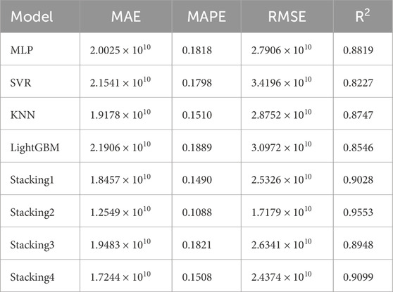
The evaluation indicators of the predictive results of four stacking models and four single models on the test dataset are presented in Table 2 and Figure 11.

Table 2

Table 2. Comparison of evaluation indicators of each model.

Figure 11

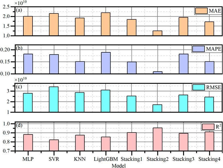
Figure 11. Comparison of evaluation indicators for four independent machine learning models (MLP, SVR, KNN, and LightGBM) and four stacking models with different structures. (a) Mean absolute error. (b) Mean absolute percentage error. (c) Root mean square error. (d) Coefficient of determination.

The predictive results for the test dataset indicate that the SVR model, when used as a meta-learner, has the optimal values for all four evaluation indicators of N_e. It achieves the highest R² value, reaching 0.9553, and the lowest values for MAE, MAPE, and RMSE, which are 1.2549 × 10¹⁰, 0.1088, and 1.7179 × 10¹⁰, respectively. Therefore, the SVR model was ultimately selected as the meta-learner for the stacking model, while the MLP, KNN, and LightGBM models were chosen as the base learners, i.e., Stacking2 in Table 1.

4.4 Model parameter

The meta-learner used in this study is SVR, and the optimizer used is the WOA. The base learners are LightGBM, KNN, and MLP. By comparing the three optimization methods (GWO, WOA, and BO), GWO was chosen to optimize them. The main parameters of each optimized model are shown in Table 3.

Table 3

Table 3. Results of each parameter of the SVR, LightGBM, KNN, and MLP models after optimization.

The main parameters of the SVR model are shown in the first row of Table 3. The parameter 1°C is the penalty parameter that controls the penalty for errors. C is positively correlated with the fitting ability of the model and also represents the probability of overfitting in the model. Gamma is the Gaussian kernel coefficient, which can control the complexity of the model. Gamma is inversely correlated with the smoothness of decision boundaries. Epsilon controls the width of the insensitive interval, and the error within this interval is accepted.

The main parameters of the LightGBM model are shown in the second row of Table 3. The feature_fraction is used to control the proportion of feature sampling used in each iteration, and its value ranges from 0 to 1. This study reduces the risk of overfitting by limiting the number of features used in each iteration while also reducing computational complexity and speeding up model training. When the data dimension is high, the role of feature_fraction is to reduce the impact of dimension disasters. The initial learning rate (base_lr) and final learning rate (final_lr) of the model are 0.0250 and 0.0060, respectively.

The main parameters of the KNN model are shown in the third row of Table 3. The number of neighbors (n_neighbors) needs to be considered when making predictions; a larger number of neighbors results in smoother model performance. The leaf_size is the size of the leaf node.

The main parameters of the MLP model are shown in the fourth row of Table 3. The MLP model used in this study adopts a configuration of one input layer, two hidden layers, and one output layer. The hidden layer nodes contain 50 and 4 nodes, respectively. The activation function used in the model is the ReLU function. The base_lr and final_lr used in the model are 0.0010 and 0.0001, respectively.

4.5 Results and analysis

After the model training is completed, we first select a period of data from m-NLP to compare the results of two methods: the stacking model and TDM, as shown in Figure 12.

Figure 12

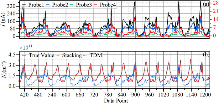
Figure 12. (a) Current collected by four probes of m-NLP. (b) Prediction results of electron density (N_e) of TDM and the stacking model.

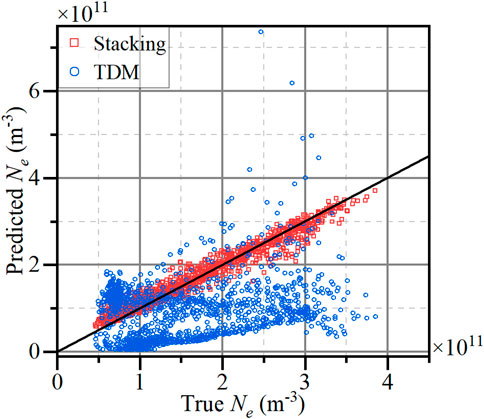
The four curves in Figure 12a correspond to the current values of the four probes, and the bias voltages corresponding to the four probes are +10V, +9V, +8V, and +6V. The red curve corresponds to the red coordinate axis on the right side, and the remaining curves correspond to the black coordinate axis on the left side. The curve in Figure 12b represents N_e corresponding to the probe current, while the black solid curve represents the N_e value obtained from IRI 2016 as the true value. The red dashed curve shows the predictive result of the stacking model, and the blue dashed curve shows the N_e diagnostic result of the TDM. The comparison of the results of the two methods is shown in Figure 13, and the distance between the results and the black curve in Figure 13 represents the error.

Figure 13

Figure 13. Deviation of the results obtained from the stacking model and TDM from the true value.

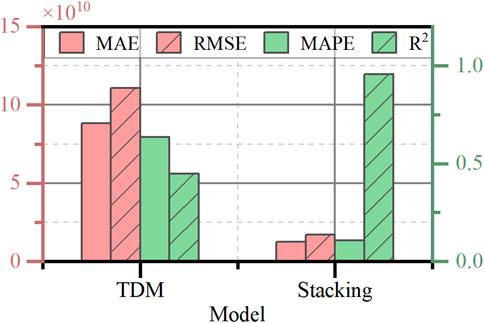
From Figures 12b, 13, the stacking model’s outcomes outperform TDM in N_e prediction, with TDM yielding consistently lower magnitude results, corroborating the findings of Hoang et al. (2018a). The difference in evaluation indicators between the two approaches is presented in Table 4 and Figure 14.

Table 4

Table 4. Comparison of evaluation indicators of the two methods.

Figure 14

Figure 14. Comparison of evaluation indicators of the stacking model and TDM.

According to Table 4, the predictive results of the stacking model are significantly better than those of the TDM in terms of evaluation indicators. The error class indicators of the stacking model, such as the MAE, MAPE, and RMSE on the test set data, are significantly lower than those of the TDM. However, the evaluation indicator R² for the stacking model fit is 0.9553, representing a significant improvement of 0.5079 compared to that of the TDM.

From Figure 12a, the data trends of probes 3 and 4 are significantly different from those of the other probes. This is mainly due to the following reasons:

• The charging effect of the spacecraft causes the voltage applied to one or several probes to be insufficient to bias the probes higher than the plasma potential.

• Pre-launch terrestrial exposure induces surface adsorbate accumulation through atmospheric oxidation processes, altering probe work function characteristics.

• One or more probes work in the plasma wake of the satellite.

• The resolution of m-NLP current measurement is 1 nA, and it has a low signal-to-noise ratio when processing weak signals.

• The probes used in m-NLP cannot satisfy the constraint relationship between the length and the Debye length.

The above reasons affect data acquisition from multiple probes, making the data unsuitable for use with the TDM and leading to certain errors in the final calculation results.

From multiple perspectives, the predictions of the stacking model are significantly better than those of the TDM and can better fit N_e of IRI 2016. This indicates that combining the stacking model with m-NLP for ionospheric plasma prediction can maintain high accuracy, even in the case of poor consistency among the currents collected by multiple probes. This method can achieve an R² of 0.9553 for N_e prediction results, proving its effectiveness as a data processing approach.

5 Conclusion

A new machine learning method has been proposed to process data from Langmuir multi-probe payloads, such as m-NLP. Due to its unique design, m-NLP can achieve high spatial resolution exploration of ionospheric irregularities, which is of great significance for the study of space weather. Nevertheless, the traditional data analysis method of Langmuir probes based on OML theory cannot be well applied to payloads such as m-NLP. This is mainly due to the following two reasons. First, the sensor used does meet the prerequisites of OML theory. For example, the probe length is significantly smaller than the Debye length, and the potential applied to the probe cannot be higher than the plasma potential. Another aspect that causes errors is the influence of the space environment. For example, the charging effect of the spacecraft creates a large potential barrier between the spacecraft and plasma, and the varying degrees of contamination between multiple probes result in poor consistency in the collection of current by the probes. The above reasons result in significant errors in the measurement of electron density using traditional analysis methods, which cannot meet the requirements for the accurate measurement of plasma.

A stacking algorithm is an integrated machine learning method that combines the prediction results of multiple base models to improve the overall prediction accuracy. It has been applied to multiple physical environments and achieved good results. The new method combines the stacking algorithm with m-NLP data for ionospheric plasma prediction, which can accurately capture the rapid changes in plasma density and help study the small-scale irregularities in the ionosphere for space weather applications. The use of machine learning methods significantly improves the prediction performance of plasma parameters compared to traditional methods based on OML. We compared and analyzed the prediction model using m-NLP data. In the case of poor consistency among the currents collected by multiple probes, the R² value of this model’s diagnostic results can reach 0.9553, which is 0.5079 higher than that of the traditional diagnostic methods.

Data availability statement

The raw data supporting the conclusions of this article will be made available by the authors, without undue reservation.

Author contributions

JW: Conceptualization, Writing – original draft, Methodology. DZ: Writing – review and editing, Formal Analysis. QZ: Supervision, Writing – review and editing, Funding acquisition. XX: Writing – original draft, Software, Formal Analysis. FZ: Writing – review and editing, Methodology. QD: Supervision, Validation, Writing – review and editing. VM: Writing – review and editing. YS: Investigation, Writing – review and editing.

Funding

The author(s) declare that financial support was received for the research and/or publication of this article. The work was supported by the National Natural Science Foundation of China (grant numbers 42325404 and 42120104003), the China Postdoctoral Science Foundation under grant number 2024M763287, and the Chinese Meridian Project.

Acknowledgments

The authors thank Zhou Yu for providing ideas and valuable discussions for this article.

Conflict of interest

The authors declare that the research was conducted in the absence of any commercial or financial relationships that could be construed as a potential conflict of interest.

Generative AI statement

The author(s) declare that no Generative AI was used in the creation of this manuscript.

Publisher’s note

All claims expressed in this article are solely those of the authors and do not necessarily represent those of their affiliated organizations, or those of the publisher, the editors and the reviewers. Any product that may be evaluated in this article, or claim that may be made by its manufacturer, is not guaranteed or endorsed by the publisher.

References

Akala, A., Doherty, P., Carrano, C., Valladares, C. E., and Groves, K. M. (2012). Impacts of ionospheric scintillations on GPS receivers intended for equatorial aviation applications. Radio Sci. 47 (04), 1–11. doi:10.1029/2012rs004995

CrossRef Full Text | Google Scholar

Allen, J. E., Boyd, R. L. F., Reynolds, P., et al. (1957). The collection of positive ions by a probe immersed in a plasma; proceedings of the proceedings of the physical society section B, F.

Google Scholar

Allen, J. J. P. S. (1992). Probe theory-the orbital motion approach. Phys. Scr. 45 (5), 497–503. doi:10.1088/0031-8949/45/5/013

CrossRef Full Text | Google Scholar

Aol, S., Buchert, S., and Jurua, E. (2020). Ionospheric irregularities and scintillations: a direct comparison of in situ density observations with ground-based L-band receivers. Earth, Planets Space 72 (1), 164. doi:10.1186/s40623-020-01294-z

CrossRef Full Text | Google Scholar

Barjatya, A., Swenson, C. M., Thompson, D. C., and Wright, K. H. (2009). Invited article: data analysis of the floating potential measurement unit aboard the international space station. Rev. Sci. Instrum. 80 (4), 041301. doi:10.1063/1.3116085

PubMed Abstract | CrossRef Full Text | Google Scholar

Bekkeng, T. A., Helgeby, E. S., Pedersen, A., Trondsen, E., Lindem, T., and Moen, J. I. (2019). Multi-needle langmuir probe system for electron density measurements and active spacecraft potential control on CubeSats. IEEE Trans. Aerosp. Electron. Syst. 55 (6), 2951–2964. doi:10.1109/taes.2019.2900132

CrossRef Full Text | Google Scholar

Bernstein, I. B., and Rabinowitz, I. N. (1959). Theory of electrostatic probes in a low-density plasma. Phys. Fluids 2 (2), 112–121. doi:10.1063/1.1705900

CrossRef Full Text | Google Scholar

Bilitza, D., Altadill, D., Zhang, Y., Mertens, C., Truhlik, V., Richards, P., et al. (2014). The international reference ionosphere 2012 – a model of international collaboration. J. Space Weather Space Clim. 4, A07. doi:10.1051/swsc/2014004

CrossRef Full Text | Google Scholar

Bridle, J. S. (1990). “Probabilistic interpretation of feedforward classification network outputs, with relationships to statistical pattern recognition,” in Neurocomputing: algorithms, architectures and applications. Springer, 227–236.

Google Scholar

Buchert, S., Zangerl, F., Sust, M., André, M., Eriksson, A., Wahlund, J., et al. (2015). SWARM observations of equatorial electron densities and topside GPS track losses. Geophys Res. Lett. 42 (7), 2088–2092. doi:10.1002/2015gl063121

CrossRef Full Text | Google Scholar

Chapin, E., Chan, S. F., Chapman, B. D., Chen, C. W., Martin, J. M., Michel, T. R., et al. (2006). “Impact of the ionosphere on an L-band space based radar,” in proceedings of the 2006 IEEE Conference on Radar (IEEE).

CrossRef Full Text | Google Scholar

Chen, F. F. (1965). Numerical computations for ion probe characteristics in a collisionless plasma. J. Nucl. Energy Part C, Plasma Phys. Accel. Thermonucl. Res. 7 (1), 47–67. doi:10.1088/0368-3281/7/1/306

CrossRef Full Text | Google Scholar

Cox, D. R. (1958). The regression analysis of binary sequences. J. R. Stat. Soc. Ser. B Stat. Methodol. 20 (2), 215–232. doi:10.1111/j.2517-6161.1958.tb00292.x

CrossRef Full Text | Google Scholar

Fish, C., Swenson, C., Crowley, G., Barjatya, A., Neilsen, T., Gunther, J., et al. (2014). Design, development, implementation, and on-orbit performance of the dynamic ionosphere CubeSat experiment mission. Space Sci. Rev. 181, 61–120. doi:10.1007/s11214-014-0034-x

CrossRef Full Text | Google Scholar

Frazier, P. I. (2018). “Bayesian optimization.” Recent advances in optimization and modeling of contemporary problems. Catonsville: Informs, 255–278.

Google Scholar

Friedrich, M., Torkar, K. M., Hoppe, U. P., Bekkeng, T. A., Barjatya, A., and Rapp, M. (2013). Multi-instrument comparisons of D-region plasma measurements. Ann. Geophys. 31 (1), 135–144. doi:10.5194/angeo-31-135-2013

CrossRef Full Text | Google Scholar

Guthrie, J., Marchand, R., Marholm, S., et al. (2021). Inference of plasma parameters from fixed-bias multi-needle langmuir probes (m-NLP). Meas. Sci. Technol. 32 (9), 095906. doi:10.1088/1361-6501/abf804

CrossRef Full Text | Google Scholar

Hoang, H., Clausen, L. B. N., Røed, K., Bekkeng, T. A., Trondsen, E., Lybekk, B., et al. (2018a). The multi-needle langmuir probe system on board NorSat-1. Space Sci. Rev. 214(4), 75. doi:10.1007/s11214-018-0509-2

CrossRef Full Text | Google Scholar

Hoang, H., RøED, K., Bekkeng, T. A., Moen, J. I., Clausen, L. B. N., Trondsen, E., et al. (2019). The multi-needle langmuir probe instrument for QB50 mission: case studies of Ex-Alta 1 and hoopoe satellites. 215: 1–19. doi:10.1007/s11214-019-0586-x

CrossRef Full Text | Google Scholar

Hoang, H., RøED, K., Bekkeng, T. A., Moen, J. I., Spicher, A., Clausen, L. B. N., et al. (2018b). A study of data analysis techniques for the multi-needle langmuir probe. Meas. Sci. Technol. 29(6): 065906. doi:10.1088/1361-6501/aab948

CrossRef Full Text | Google Scholar

Hoskinson, A., and Hershkowitz, N. (2006). Effect of finite length on the current–voltage characteristic of a cylindrical langmuir probe in a multidipole plasma chamber. Plasma Sources Sci. Technol. 15 (1), 85–90. doi:10.1088/0963-0252/15/1/013

CrossRef Full Text | Google Scholar

Ivarsen, M. F., Hoang, H., Yang, L., Clausen, L. B. N., Spicher, A., Jin, Y., et al. (2019). Multineedle langmuir probe operation and acute probe current susceptibility to spacecraft potential. IEEE Trans. Plasma Sci.. 47(8): 3816–3823. doi:10.1109/TPS.2019.2906377

CrossRef Full Text | Google Scholar

Jacobsen, K., Pedersen, A., Moen, J., and Bekkeng, T. A. (2010). A new langmuir probe concept for rapid sampling of space plasma electron density. Meas. Sci. Technol. 21 (8), 085902. doi:10.1088/0957-0233/21/8/085902

CrossRef Full Text | Google Scholar

Jakowski, N., Wehrenpfennig, A., Heise, S., Schlueter, S., and Noack, T. (2001). “Space weather effects in the ionosphere and their impact on positioning,” in Proceedings of the ESA workshop paper, F.

Google Scholar

Ke, G., Meng, Q., Finley, T., Wang, T., Chen, W., Ma, W., et al. (2017). Lightgbm: a highly efficient gradient boosting decision tree. Adv. neural Inf. Process. Syst., 30.

Google Scholar

Kintner, P. M., and Ledvina, B. M. (2005). The ionosphere, radio navigation, and global navigation satellite systems. AdSpR 35 (5), 788–811. doi:10.1016/j.asr.2004.12.076

CrossRef Full Text | Google Scholar

Kintner, P. M., and Seyler, C. E. (1985). The status of observations and theory of high latitude ionospheric and magnetospheric plasma turbulence. Space Sci. Rev. 41 (1), 91–129. doi:10.1007/bf00241347

CrossRef Full Text | Google Scholar

Krizhevsky, A., Sutskever, I., and Hinton, G. E. (2017). ImageNet classification with deep convolutional neural networks. Commun. ACM. 60 (6), 84–90. doi:10.1145/3065386

CrossRef Full Text | Google Scholar

Kruse, R., Mostaghim, S., Borgelt, C., Braune, C., and Steinbrecher, M. (2022). Multi-layer perceptrons [M]. Computational intelligence: a methodological introduction. Springer, 53–124.

Google Scholar

Lebreton, J.-P., Stverak, S., Travnicek, P., Maksimovic, M., Klinge, D., Merikallio, S., et al. (2006). The ISL langmuir probe experiment processing onboard DEMETER: scientific objectives, description and first results. Planet. Space Sci. Instrum. 54 (5), 472–486. doi:10.1016/j.pss.2005.10.017

CrossRef Full Text | Google Scholar

Lecun, Y., Bottou, L., Orr, G. B., and Müller, K.-R. (2002). Efficient backprop [M]. Neural networks: tricks of the trade. Springer, 9–50.

Google Scholar

Lee, J. C., Min, K. W., Ham, J., Kim, H., and Hong, S. (2013). Langmuir probe experiments on Korean satellites. CAP 13 (5), 846–849. doi:10.1016/j.cap.2012.12.011

CrossRef Full Text | Google Scholar

Liu, G., Marholm, S., Eklund, A. J., Clausen, L., and Marchand, R. (2023). m-NLP inference models using simulation and regression techniques. J. Geophys. Res. Space Phys. 128 (2), e2022JA030835. doi:10.1029/2022ja030835

PubMed Abstract | CrossRef Full Text | Google Scholar

Liu, Y., Zhou, C., Xu, T., Tang, Q., Deng, Z., Chen, G., et al. (2021). Review of ionospheric irregularities and ionospheric electrodynamic coupling in the middle latitude region. EARTH Planet. Phys. 5 (5), 1–21. doi:10.26464/epp2021025

CrossRef Full Text | Google Scholar

Marholm, S., Marchand, R., Darian, D., Miloch, W. J., and Mortensen, M. (2019). Impact of miniaturized fixed-bias multineedle langmuir probes on cubesats. ITPS 47 (8), 3658–3666. doi:10.1109/tps.2019.2915810

CrossRef Full Text | Google Scholar

Mienye, I. D., and Sun, Y. (2022). A survey of ensemble learning: concepts, algorithms, applications, and prospects. IEEE Access 10, 99129–99149. doi:10.1109/access.2022.3207287

CrossRef Full Text | Google Scholar

Mirjalili, S., and Lewis, A. (2016). The whale optimization algorithm. Adv. Eng. Softw. 95, 51–67. doi:10.1016/j.advengsoft.2016.01.008

CrossRef Full Text | Google Scholar

Mirjalili, S., Mirjalili, S. M., and Lewis, A. (2014). Grey wolf optimizer. Adv. Eng. Softw. 69 (3), 46–61. doi:10.1016/j.advengsoft.2013.12.007

CrossRef Full Text | Google Scholar

Mott-Smith, H. M., and Langmuir, I. (1926). The theory of collectors in gaseous discharges. Phys. Rev. 28 (4), 727–763. doi:10.1103/physrev.28.727

CrossRef Full Text | Google Scholar

Ning, B., Hu, L., Li, G., Liu, L., and Wan, W. (2012). The first time observations of low-latitude ionospheric irregularities by VHF radar in Hainan. Sci. China Technol. Sci. 55, 1189–1197. doi:10.1007/s11431-012-4800-2

CrossRef Full Text | Google Scholar

Reid, G. C. (1968). The formation of small-scale irregularities in the ionosphere. J. Geophys Res. 73 (5), 1627–1640. doi:10.1029/ja073i005p01627

CrossRef Full Text | Google Scholar

Ribeiro, M. H. D. M., and Dos Santos Coelho, L. (2020). Ensemble approach based on bagging, boosting and stacking for short-term prediction in agribusiness time series. Appl. soft Comput. 86, 105837. doi:10.1016/j.asoc.2019.105837

CrossRef Full Text | Google Scholar

Smola, A. J., and SchöLKOPF, B. (2004). A tutorial on support vector regression. Stat. Comput. 14, 199–222. doi:10.1023/B:STCO.0000035301.49549.88

CrossRef Full Text | Google Scholar

Tereshchenko, E., Khudukon, B., Rietveld, M., Isham, B., Hagfors, T., and Brekke, A. (2006). “The relationship between small-scale and large-scale ionospheric electron density irregularities generated by powerful HF electromagnetic waves at high latitudes,” in Proceedings of the AnGeo, F (Germany: Copernicus Publications Göttingen).

Google Scholar

University of Olso (2024). NorSat-1 multi-needle langmuir probe data. Available online at: http://tid.uio.no/plasma/norsat/index.html (Accessed March 20, 2024).

Google Scholar

Wang, X., Samaniego, J., Hsu, H. W., Horányi, M., Wahlund, J., Ergun, R. E., et al. (2018). Development of a double hemispherical probe for improved space plasma measurements. J. Geophys. Res. Space Phys. 123 (4), 2916–2925. doi:10.1029/2018ja025415

CrossRef Full Text | Google Scholar

Xing, Z., Zhang, Q., Han, D., Zhang, Y., Sato, N., Zhang, S., et al. (2018). Conjugate observations of the evolution of polar cap arcs in both hemispheres. J. Geophys. Res. Space Phys. 123 (3), 1794–1805. doi:10.1002/2017ja024272

CrossRef Full Text | Google Scholar