Design and performance characterization of H-band MCT camera: insights from pixel-level gain measurements

Infrared astronomical equipment is pivotal in advancing our understanding of the universe, particularly through ground-based observations, which remain the primary mode of astronomical study. In this paper, we introduce the development and performance characterization of an H-band Mercury Cadmium Telluride (MCT) infrared camera designed for astronomical observations. We computed the photon transfer curve (PTC) for each pixel and fitted these curves to derive pixel-level gain. The results reveal a spatial non-uniformity of detector pixel-level gain, which correlates with changes in field of view (FOV). By employing FOV compensation, we achieved more uniform gain distribution. This testing approach allows for a more accurate performance evaluation of scientific-grade astronomical cameras, providing a robust foundation for subsequent astronomical image analysis and benefiting the field of infrared astronomy.

1 Introduction

Understanding the physical processes of galaxy evolution is one of the most prominent issues in contemporary astronomy. Galaxy formation and evolution are driven by star formation, galactic mergers, and secular evolution over cosmic time scales (Conselice et al., 2014). Morphologically, galaxies evolve from irregular or peculiar systems at redshifts z > 1 into more regular structures at lower redshifts (Mortlock et al., 2013). Infrared observations play a crucial role in unraveling these mechanisms, as they can probe dust-enshrouded regions of star formation, as well as distant and faint celestial objects.

As most of the infrared radiation emitted by celestial bodies is absorbed by Earth’s atmosphere, this necessitates the use of ground-based infrared telescopes through specific atmospheric windows, such as the J, H, and K bands (Simons and Tokunaga, 2002), shown in Figure 1. Antarctica, particularly the Kunlun Station (Dome A), is one of the best locations on Earth for infrared and submillimeter astronomical observations due to exceptional seeing conditions and atmospheric stability (Ma et al., 2020). Under typical Antarctic sky background levels in the H band (1,100–2,600 μJ y/arcsec²) (Zhang et al., 2023), a telescope system with a 41 cm aperture, f/2.5 optics, and 15-μm-pixel size is expected to receive approximately 3,243–7,670 photoelectrons per pixel per second from the sky background. To operate in a background-limited regime, the detector’s readout noise must remain below the square root of this signal level, i.e., less than 50 e⁻ per pixel.

Figure 1

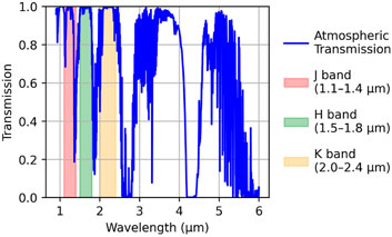
Figure 1. Near-infrared atmospheric transmission.

The materials commonly used in infrared detector include InSb, InAs/GaSb, and InGaAs, each offering distinct advantages and limitations in spectral coverage and noise characteristics. InSb detectors have the good performance across in the band of 1–5 μm range with low readout noise between 10 and 30 electrons at 77 K, but its higher dark current in the H-band between 1.5 and 1.8 μm limits its applications (Rayner et al., 2003). InAs/GaSb superlattice detectors, typically optimized for the mid-infrared wavelengths from 3 to 5 μm, exhibit relatively high noise levels of 50–100 electrons at shorter wavelengths (Rogalski, 2017). InGaAs detectors provide moderate noise levels of 20–40 electrons and can be operated in the cooling temperature near 180 K, but their quantum efficiency rapidly declines beyond approximately 1.68 μm, limiting their effectiveness for full H-band coverage (Ofer et al., 2021).

By comparison, Mercury Cadmium Telluride (MCT) detectors, noted for their high quantum efficiency and low dark current (Rogalski, 2020), are widely preferred for high-performance infrared astronomical detection and have been employed in major space missions such as Euclid (Waczynski et al., 2016) and the Nancy Grace Roman Space Telescope (Mosby Jr et al., 2020). The WIRCam imager on CFHT (Puget et al., 2004) or HAWK-I on the VLT (Kissler-Patig et al., 2008), equipped with Teledyne HAWAII-2RG (H2RG) or H4RG focal plane arrays, routinely achieve low readout noise (as low as 5–12 e⁻), dark current below 0.1 e⁻/s/pixel at 77K. However, such detectors or devices are currently restricted from being imported to China, which motivates the development and deployment of scientific-grade MCT detectors in China. Recent progress in Chinese MCT detector development (Xin et al., 2022), particularly at the Shanghai Institute of Technical Physics (SITP), has led to devices suitable for scientific-grade ground-based infrared astronomy (Liang et al., 2024). In contrast to existing large-scale observatory cameras, the presented system offers a compact, power-efficient (∼45 W total), and modular alternative specifically tailored for extreme environments like Dome A.

In this paper, we introduce the development of an H-band infrared camera equipped with a 640 × 512 MCT detector from SITP, designed specifically for observation in Antarctica. The camera is designed for observation of low-temperature celestial objects (e.g., brown dwarfs and planetary nebulae) and high-redshift galaxies. Leveraging Dome A’s low sky brightness and reduced thermal noise, the camera is expected to deliver image quality that, in some respects, surpasses that of the 2MASS survey (Skrutskie et al., 2006), particularly in terms of spatial resolution and detector linearity.

In addition, in this article the characteristics and correction strategies of its pixel level detector are presented. A pixel-level gain (PLG) mapping methodology is developed based on analysis of photon transfer curve (PTC), enabling precise quantification of gain non-uniformity across the array of whole detector. Furthermore, we identify a systematic spatial dependence of gain associated with the pixel field-of-view (FOV) angle. This effect is modeled and compensated using a geometric correction approach, significantly improving the spatial uniformity of gain.

In this paper, it is structured as follows: in Section 2 we introduce the optics, mechanics, and electronics of our MCT camera. In Section 3 we detail the methodology and results of PLG characterization and FOV-based correction. In Sections 4 and 5, we present the field test results and summarize the broader implications of this work.

The key contributions of this article are summarized as follows:

1. Development of a low-noise H-band infrared camera utilizing a MCT detector made in China, tailored specifically for ground-based astronomical observations in Antarctica.

2. Introduction of a PLG measurement approach that reveals a spatial correlation between gain non-uniformity and the FOV angle, along with a geometric compensation method that improves the spatial uniformity of detector gain.

2 Design of the H-band MCT camera

The design of the H-band MCT camera was driven by the requirements of astronomical observations in Antarctica, with careful design of optics, detectors, and system-level components to ensure optimal performance.

2.1 Optics of the telescope

The optical design was tailored to match a 41-cm aperture f/2.5 telescope of Sun Yat-sen University, as shown in Figure 2. Given the relatively higher readout noise and dark current of the detector compared to leading international detectors, minimizing additional noise sources—particularly stray light and optical efficiencies—is crucial to fully exploit the exceptionally low infrared sky background at Dome A. To maximize optical throughput in H band while suppressing off-axis thermal radiation and unwanted reflections, a cold shield and a custom-designed H-band filter were incorporated, significantly limiting background flux and enhancing image contrast.

Figure 2

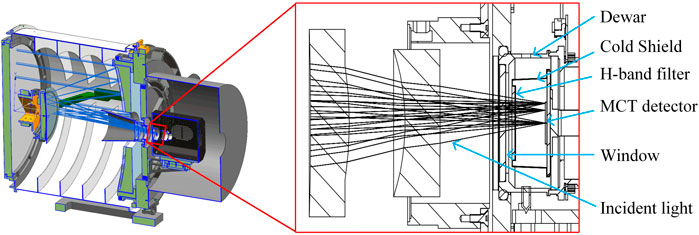
Figure 2. Diagram of the optical assembly of a 41-cm-aperture telescope with a MCT camera.

The camera’s FOV reaches approximately 0.5 × 0.4 square degrees (f/0.6), fully utilizing the telescope’s image field without significant vignetting or peripheral aberrations. Figure 3 illustrates the transmittance curves of the camera’s filter and window at room temperature (300 K), compared with atmospheric transmission.

Figure 3

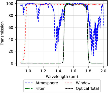
Figure 3. Transmittance of the filter and window.

2.2 System architecture of H-band MCT camera

The camera employs a 640 × 512 MCT focal plane array developed by SITP (see Figure 4a). The detector features a pixel pitch of 15 µm and a cutoff wavelength of 2.0 µm, covering the full H-band atmospheric window. The detector adopts a hybrid structure in which a MCT layer is bump-bonded to a silicon readout integrated circuit (ROIC) chip with indium pillars (see Figure 4b). This hybrid integration method provides robust mechanical performance and reliable electrical interconnectivity under thermal cycling conditions (Zhang et al., 2012). Additionally, careful thermal management during cryogenic characterization tests has demonstrated stable detector performance at low temperatures (Jiménez et al., 2020; Stoyanov et al., 2019).

Figure 4

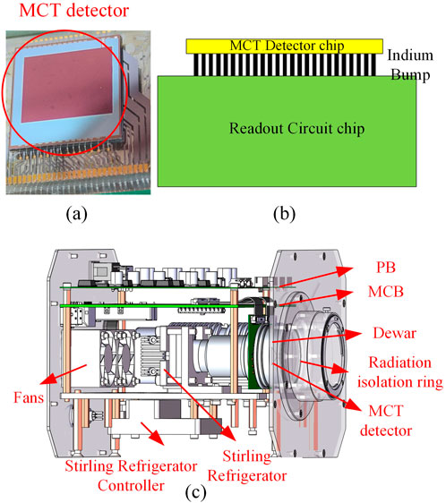
Figure 4. MCT detectors from SITP and the structure of H-band camera: (a) Picture of the MCT detector, (b) Stacking structure of the detector, (c) The structure of the H-band camera.

In the H-band camera, the optics and detector components were integrated into a vacuum-sealed Dewar, which is cooled to approximately 80 K by a Stirling-cycle cryocooler (see Figure 4c). The Dewar employs an aluminum nitride (AlN) mounting plate for both mechanical support and efficient thermal conduction. Electrical connections to the external readout electronics are made via gold wire bonds and routed through hermetically sealed feedthroughs.

Given the extremely low ambient temperatures at Dome A, typically below −60°C, a heating film is integrated into the system to maintain the refrigeration unit’s operational range above −40 °C. To prevent thermal infrared radiation from the heater affecting the detector’s photosensitive surface, a radiation isolation ring is installed between the Dewar window and outer shell, effectively blocking internal thermal emissions from reaching the focal plane.

The readout circuit in the MCT detector is a capacitive transimpedance amplifier (CTIA) architecture, which is operated in reduced bandwidth and incorporated two selectable integration capacitance modes for gain selection, 5 fF and 10 fF (see Figure 5). With reset after integration time, the response electrons of each pixel are integrated and converted into voltage signals. After sampling, the signals are selected by rows and columns, and the array pixel signals are transmitted to the output stage one by one, and finally output outside the chip.

Figure 5

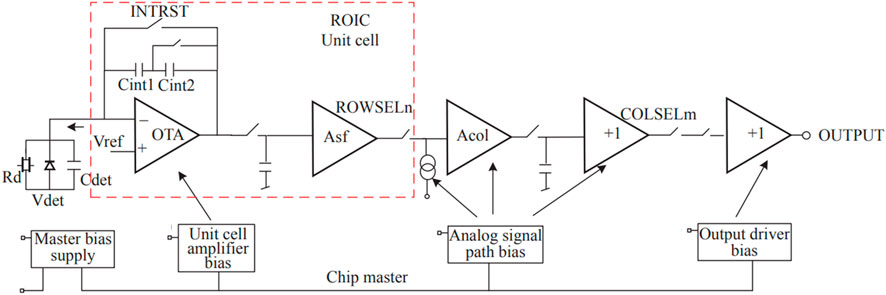
Figure 5. The readout circuit in the MCT detector (Liang et al., 2024).

The electronics of the camera consists of a Main Control Board (MCB) and a Power Board (PB). The MCB handles system control, readout, and data processing, while the PB provides power and manages temperature control through a heating module. The functional diagram of the H-band camera is shown in Figure 6. To enhance operational robustness under remote and harsh conditions, the camera supports dual communication interfaces (UDP and USB 2.0). The UDP interface is typically preferred due to its longer transmission distance, but the USB link provides a redundant fallback channel in case of network disruptions. The total power consumption including the cryocooler and all electronics, is approximately 45 W. This low-power design is particularly well-suited for autonomous and long-term deployment at Dome A, where both power availability and thermal balance are critical constraints.

Figure 6

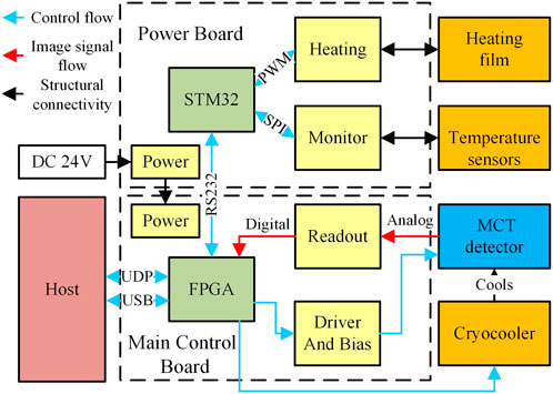
Figure 6. Functional Diagram of the electronics in the H-band Camera.

The detector signal passes through an ADC driver with a gain of 1.667—selected to match the input dynamic range—and is sampled by an 18-bit ADC. An FPGA then transmits the upper 16-bit data to the host computer (see Figure 7) for maximizing dynamic range.

Figure 7

Figure 7. Diagram of readout module.

2.3 Performance characterizations

Comprehensive performance characterization is essential for scientific-grade infrared cameras, especially when deployed in extreme environments such as Antarctica (Sutherland et al., 2015; Zhang et al., 2019). These tests provide quantitative validation of the camera’s readiness for high-fidelity imaging under low-background infrared conditions (Tubiana et al., 2015).

A dedicated test platform was established for this purpose, as illustrated in Figure 8. A critical component of the test setup is the blackbody radiation source, which directly influences the accuracy of detector calibration (Qu et al., 2025; Wright et al., 2015). The blackbody source features a 100 mm emission surface, temperature control precision of ±0.02°C, resolution of 0.01°C, and temperature stability better than 0.1°C per 10 min. During testing, the camera was precisely aligned so that all pixels viewed only the blackbody surface, thereby minimizing stray radiation. Under conditions of assumed uniform blackbody emission, the illumination non-uniformity across the detector’s field of view was measured to be ∼3.74%.

Figure 8

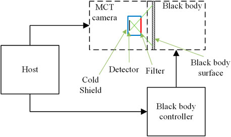
Figure 8. The test platform for the MCT camera.

The photon transfer curve (PTC) method was employed to evaluate gain for both the central 40 × 40 pixels region and the entire detector area (see Figure 9) (Sun et al., 2022). For the 5 fF integration capacitor, the measured gains are 1.04 e⁻/ADU and 1.13 e⁻/ADU in these two different area, where ADU denotes an analog-to-digital unit. At a setting of 5 fF, the measured readout noise is approximately 29.8 e⁻, and the readout electronics contributed about 5.5 e⁻, indicating that the main noise component is inside the detector. According to the standard of response rate less than 50% and greater than 200%, the proportion of bad pixels is 0.44%

Figure 9

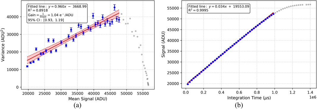
Figure 9. Flat field test of 40 × 40 pixels in the central area: (a) Photon transfer curve (PTC), where the gain is calculated as the reciprocal of the slope; the shaded area represents the confidence interval (CI). (b) Photon response curve, from which response linearity and full well capacity can be derived. ADU denotes analog-to-digital unit.

Inter-pixel capacitance (IPC) estimation is based on the spatial autocorrelation function (ACF) approach (Moore et al., 2004). We first subtract the mean from each image to obtain zero-mean data, and then calculate the two-dimensional ACF using Fast Fourier Transform (FFT). The central peak of the ACF is normalized to unity, and the IPC is estimated by averaging the autocorrelation values of the four nearest-neighbor pixels adjacent to the central peak, as shown in Figure 10. The derived IPC value was below 0.01, suggesting a negligible influence on gain estimation. Therefore, IPC correction was not applied in this analysis. While IPC may affect the Point spread function (PSF) in precision photometry, accurate correction would require a full-system model including optical aberrations and on-sky PSF measurements (Kannawadi et al., 2016), which are outside the scope of the present laboratory characterization and are planned for future work.

Figure 10

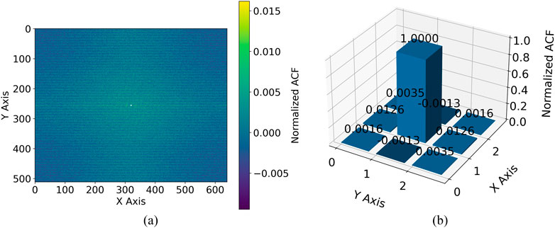
Figure 10. Estimation of Inter pixel Capacity Impact. (a) Two-dimensional autocorrelation function (ACF) of the detector image, with the central 3 × 3 pixels region masked to highlight neighboring pixel correlations for interpixel capacitance (IPC) estimation. (b) Three-dimensional bar plot of normalized ACF values in the central 3 × 3 pixels region, illustrating the strength of pixel-to-pixel correlation caused by IPC effects.

Since the detector was already sealed within a Dewar, conventional dark current measurement using a cold shutter is not feasible. As an alternative, the camera was placed in a refrigerated environment to reduce the ambient photon flux, enabling an approximate evaluation under dark-field conditions. At a stabilized temperature of −25°C, the longest exposure time of the camera exceeds 20 min, and the incident background in the H-band was estimated to be approximately 9 photons per second per pixel, while the measured signal slope was approximately 17 electrons per second per pixel. This value reflects the combined contributions from the detector’s intrinsic dark current, residual ambient background radiation, and readout noise.

PRNU was measured to be 4.44% using flat-field illumination at various exposure times. The Signal-to-Noise Ratio increases markedly with higher illumination, reaching a maximum of about 135 (42.60 dB) before the detector approaches full well capacity. Based on a comparative analysis with the 2MASS system, which achieved a limiting magnitude of H ≈ 15.1 at SNR = 10 using a 1.3 m f/3.5 telescope and a ∼7.8 s exposure per scan, we estimate the limiting magnitude of our 0.41 m f/2.5 system under Dome A conditions to be approximately 12.8 mag for a 10 s exposure at the same SNR level. With frame stacking or extended exposures up to 60 s, the limiting magnitude would be expected to improve to 14.0–14.3, demonstrating the system’s capability to detect faint astronomical sources under background-limited conditions.

3 PLG testing and FOV impact

The precise gain measurement of a detector is crucial for the accurate characterization of its performance. Gain represents the conversion factor between the detection signal and the output of a detector, which serves as a fundamental parameter for explaining a detector’s response to incident radiation and plays a crucial role in calculating other performance parameters (Janesick, 2007). Consequently, PLG measurement provides deeper insights into detector performance and scientific calculation.

3.1 Defects of PTC method

In an ideal PTC measurement, it is assumed that each pixel in the detector follows the same Poisson distribution for every acquisition. In reality, the mean photon count for each pixel is not identical. For pixel i, its Poisson mean is ${\mathrm{\lambda }}_i$, which can vary depending on the pixel’s FOV angle—pixels with a larger FOV angle collect more photons, and vice versa.

Consequently, if one treats all pixels as a single ensemble when estimating the “variance vs mean,” this is equivalent to randomly selecting a pixel i with probability 1/N (where N = 640 × 512), and then drawing a single observation from Poisson (${\lambda }_i$). From the perspective of mixed distributions, the random variable $X_{mix}$ (formed by mixing measurements across all pixels) has the following expectation and variance, refer to the appendix for details. Equations 1, 2 show the mathematical expectation and variance of X_mix, respectively:

$E\left[X_{mix}\right]=\frac{1}{N}{\displaystyle \sum _{i=1}^N}{\lambda }_i,(1)$

$Var\left(X_{mix}\right)=\underset{MeanPoissonvariance}{\underbrace{\frac{1}{N}{\displaystyle \sum _{i=1}^N}Var\left(Poisson\left({\lambda }_i\right)\right)}}+\underset{Nonuniformdistribution}{\underbrace{Var\left({\lambda }_i\right)}}=\frac{1}{N}{\displaystyle \sum _{i=1}^N}{\lambda }_i+Var\left({\lambda }_i\right),(2)$

For a Poisson distribution with parameter ${\lambda }_i$, the variance is ${\lambda }_i$ Hence the first term represents the average of the Poisson variances of the pixels, while the second term is the “extra mixture variance” caused by differences in the pixel means. Defining Equation 3 as follows,

$\overline{\lambda }=\frac{1}{N}{\displaystyle \sum _{i=1}^N}{\lambda }_i,{\sigma }_{\lambda }^2=Var\left({\lambda }_i\right),(3)$

we obtain the simplified variance formula in Equation 4,

$var\left[X_{mix}\right]=\overline{\lambda }+{\sigma }_{\lambda }^2,(4)$

Accordingly, we define the variance-to-mean ratio in Equation 5 as:

$\frac{var\left(X_{mix}\right)}{\overline{X_{mix}}}=\frac{\overline{\lambda }+{\sigma }_{\lambda }^2}{\overline{\lambda }}=1+\frac{{\sigma }_{\lambda }^2}{\overline{\lambda }},(5)$

The standard PTC method assumes all pixels follow Poisson (${\lambda }_i$) with the same $\lambda$. Under this assumption, $var\left(X_{mix}\right)\approx g\times X_{mix}$, and a linear fit to $var\left(X_{mix}\right)\text{\hspace{0.17em}vs}.X_{mix}$ yields the slope $g$. In practice, though, the slope is (Equation 6) becames:

$Slope=\frac{var\left(X_{mix}\right)}{\overline{X_{mix}}}=g+\frac{{\sigma }_{\lambda }^2}{\overline{\lambda }g}>g\left(\text{unless\hspace{0.17em}all\hspace{0.17em}}{\lambda }_i\text{are\hspace{0.17em}identical}\right),(6)$

leading to a fitted gain higher than the detector’s true gain.

3.2 PLG testing

The photon transfer curve method is employed to calculate pixel gain by analyzing the linear relationship between the mean signal and variance of flat-field images at different exposure times. This method involves capturing 400 × 50 flat-field images, where 400 denotes the number of frames taken for each exposure time $t_i$ and 50 represents the number of different exposure times.

For each pixel $\left(x,y\right)$, the mean signal $S_{\left(x,y\right)}\left(t_i\right)$ and noise variance ${\mathrm{\sigma }}_{\left(x,y\right)}^2\left(t_i\right)$ are calculated using Equations 7, 8, respectively:

$S_{\left(x,y\right)}\left(t_i\right)=\frac{1}{n}{\displaystyle \sum _{j=1}^n}{I}_{\left(x,y\right)}\left(t_i,j\right),(7)$

${\mathrm{\sigma }}_{\left(x,y\right)}^2\left(t_i\right)=\frac{1}{n-1}{\displaystyle \sum _{j=1}^n}{\left(I_{\left(x,y\right)}\left(t_i,j\right)-S_{\left(x,y\right)}\left(t_i\right)\right)}^2,(8)$

Where $I_{\left(x,y\right)}\left(t_i,j\right)$ is the signal value of pixel $\left(x,y\right)$ in the jth frame under exposure time $t_i$.By plotting ${\mathrm{\sigma }}_{\left(x,y\right)}^2\left(t_i\right)$ against $S_{\left(x,y\right)}\left(t_i\right)$, a linear PTC response is obtained.

Pixel-level gain testing was conducted across two experimental setups, and obtained a flat and regular gain distribution on the testing platform with an optical system, which conforms to the gain inconsistency phenomenon caused by CMOS readout circuit process deviation and has obvious horizontal and vertical patterns. For the test results of H-band cameras without optical lenses, the horizontal and vertical distribution of gain cannot be observed, highlighting the central circular distribution, as shown in Figure 11. The pixel level gain has been normalized, according to Equation 9 and the gain calculated based on the PTC is set to 1.

${gain}_{Normalized}={gain}_{Pixel-level}/{gain}_{PTC},(9)$

Figure 11

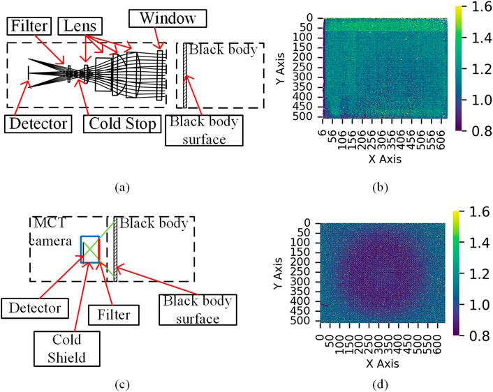
Figure 11. The results of Single pixel gain tests: (a,b) Test platform with an optical system and test results, (c,d) Test platform and test results of our camera.

The heatmap in Figure 11 reveals a consistent pattern: the central region of the detector exhibits lower normalized gain values, while higher values are observed toward the periphery. Importantly, since the PLG method relies on photon shot noise statistics and is independent of the absolute illumination level (assuming Poisson-distributed incident light), these spatial variations cannot be attributed to vignetting, stray light, or illumination gradients. To further investigate this trend, as shown in Figure 12a, the x-axis represents coordinates from the center, and the y-axis represents the ${gain}_{Normalized}$. There are 95% of pixel-gain points between the red and green lines. The gain distribution at a distance of 200 pixels from the center as shown in Figure 12b. Kernel Density Estimation (KDE) is a non-parametric method used to estimate an unknown probability density function (Silverman, 2018), the distribution is basically consistent with a Gaussian distribution.

Figure 12

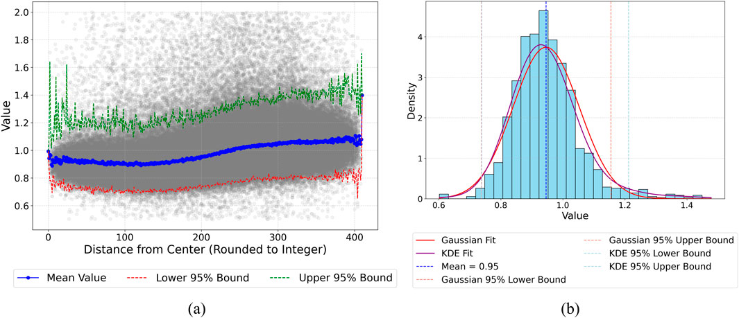
Figure 12. Analysis of Pixel-Level Gain Variations Across the Detector: (a) Pixel-Level Gain Variation at Different Distances from the Center, (b) Pixel-Level Gain Distribution at distance of 200 Pixels from the Center.

3.3 Impact of FOV on gain uniformity

Testing systems with optical lenses have more regular pixel level gains for detectors, while detectors in H-band cameras may not receive uniform incident light due to different fields of view, which may affect the measurement results of pixel level gains. We propose a geometric FOV compensation method to mitigate pixel-level gain non-uniformity.

Pixel A is a point on the detector, as shown in Figure 13a, and the conical surface formed by point A along the cold screen hole is the solid angle at which pixel A can receive radiation, Figure 13b shows the cross-section along the XOZ plane. Based on the cross-section, AE is the angle bisector of angle BAC, and point E is the intersection point of this angle bisector and the cold screen hole plane. Therefore, based on geometric relationships, we calculate parameters e, f, and s using Equations 10–12, respectively

$e=\sqrt{bc\left({\left(b+c\right)}^2-a^2\right)}/\left(a+c\right),(10)$

$f=\sqrt{2\left(b^2+c^2\right)+a^2}/2,(11)$

$s=g-\sqrt{e^2-h^2},(12)$

Figure 13

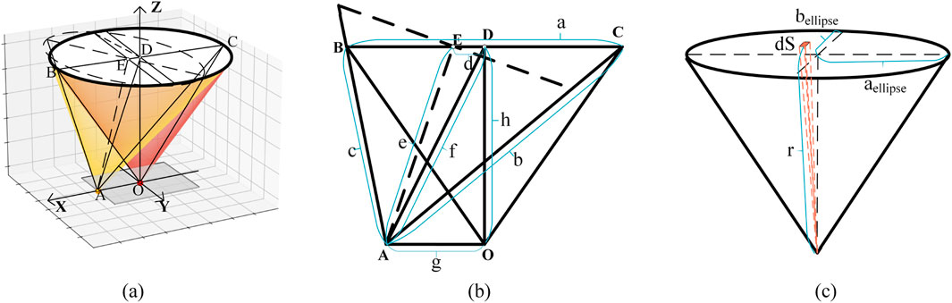
Figure 13. Illustration of the solid angle: (a) The FOV angles for the detector center and edge points; (b) Cross-sectional view of the solid angle; (c) Illustration of the calculation of the solid angle for an elliptical cone.

We convert the oblique elliptical cone surface of the solid angle of point A into a regular elliptical cone surface with AE , as shown in Figure 13c and the lengths of its major and minor axes can be calculated according to Equations 13, 14

$a_{ellipse}=\sqrt{{\left(a/2\right)}^2-s^2},(13)$

$b_{ellipse}=e\tan \left(A/2\right),(14)$

Calculate the solid angle numerically based on the height of the regular elliptical cone and the length of the major and minor axes of the ellipse (Li et al., 2012), as described by Equation 15.

$\mathrm{\Omega }=\int \frac{dS}{r^2},(15)$

The solid angles of light windows vary across different pixel locations on the detector, resulting in a discrepancy in the number of photons received by pixels at different positions. We consider the central area of the detector as the most important observation area, therefore the circular area at the center is designated as area A, the circular area to the X-axis boundary is designated as area B, and the surrounding corners are designated as area C. As shown in Figure 14, it can be observed that the variation in the solid angle is minimal within the central region (Region A), while it decreases significantly as the pixels approach the edge of the detector. The normalization and subsequent pixel-level gain corrections are implemented using Equations 16, 17: The normalized field-of-view (FOV) coefficient and the parameter for pixel-level gain correction are calculated using Equations 16, 17 respectively:

${FOV}_{Normalized}=FOVValue/\overline{FOVValue},(16)$

${gain}_{NormalizedCorrected}={gain}_{Normalized}\times {FOV}_{Normalized},(17)$

Figure 14

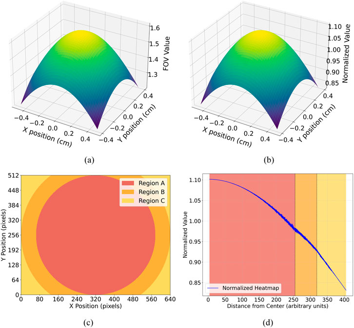
Figure 14. Variation of FOV angles across different pixel positions: (a) Comparison FOV angles between the center and corner positions, (b) FOV angles at various positions, normalized by the average, (c) Division of the detector into three regions based on distance from the central area, (d) Plot of FOV angle versus distance from the center.

The pixel gain was corrected according to Equation 18, yielding a curve representing the average gain as a function of the distance from the center of the detector, as shown in Figure 15a. In regions A and B, the corrected gain remains approximately constant at a value of 1 (∼ ${gain}_{PTC}$). After using FOV correction, the detector gain is basically consistent in the central area, close to the overall calculated gain value, while the gain value in the corner area is smaller.

$Correctedgain={gain}_{NormalizedCorrected}\times {gain}_{PTC},(18)$

Figure 15

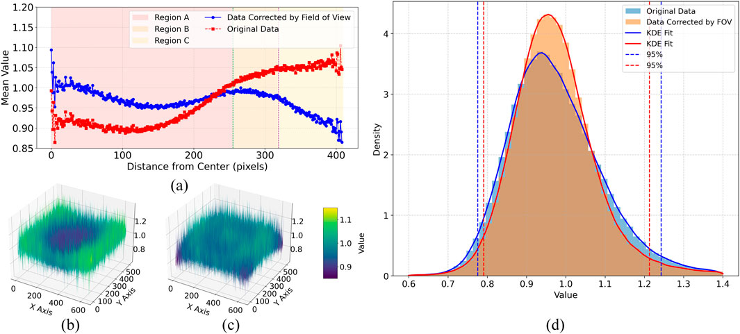
Figure 15. Comparison of pixel gain distribution before and after FOV correction: (a) Pixel gain as a function of distance from the central position, (b) 3D distribution of the original pixel gain, (c) 3D distribution of the corrected pixel gain, and (d) histogram illustrating the statistical distribution of pixel gain.

According to the calculation of the average values of pixels before and after correction based on three partitions, as shown in Figure 16, it can be concluded that using pixel level correction can make the spatial distribution of gain more uniform. This indicates that the different fields of view of the detector may have a correlation with the pixel level gain calculation method.

Figure 16

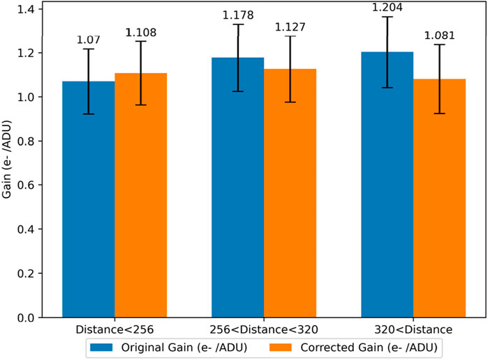
Figure 16. Bar chart comparing the original and corrected gain values (in e⁻/ADU) across three regions with different distance ranges, Error bars represent the standard deviation of the gain measurements.

4 Field test

In our camera system, particular emphasis is placed on the central region due to its significantly lower density of defective pixels compared to the edges. Upon observing non-uniformity in the gain spatial distribution, it becomes necessary to recalibrate the performance metrics specifically within this central area, using the average gain value of Region A, are shown in Table 1.

Table 1

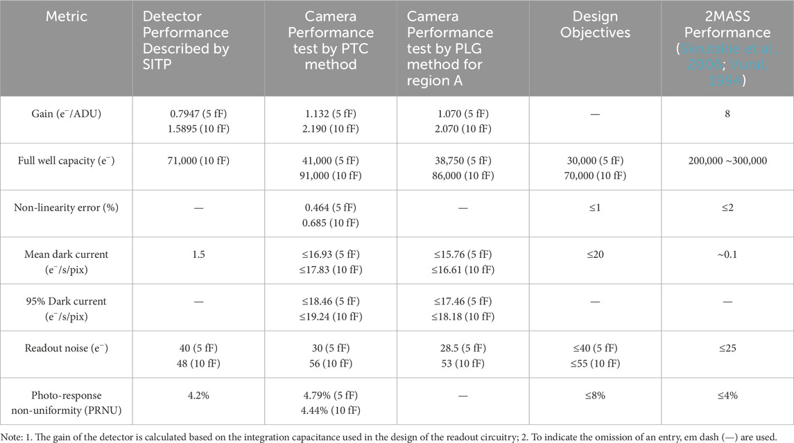
Table 1. Comparative performance metrics.

The H-band MCT camera was integrated with the 41 cm telescope and deployed at Daocheng Observatory (29°03′14″N, 100°17′56″E) for preliminary on-sky testing. As shown in Figure 17, this test aimed to validate system-level functions such as mechanical stability, thermal regulation, optical alignment, and detector readout integration. During this test, near-infrared images of the Orion Nebula (M42) were captured to confirm optical throughput and basic imaging capability. While the acquired data were not intended for scientific analysis, they demonstrate the system’s readiness for astronomical observations, including potential deployment at Dome A.

Figure 17

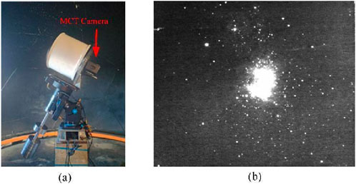
Figure 17. Field test At DaoCheng Observatory: (a) Telescope and Camera Setup, (b) Composite Image from Multiple Exposures.

5 Conclusion

In this study, we presented the design, integration, and performance characterization of a 640 × 512 pixels MCT infrared camera tailored for ground-based H-band astronomical observations. The focal point of the evaluation was the PLG analysis and its correlation with the FOV angle across the detector. By accounting for variations in the pixel incident solid angle, we corrected for gain non-uniformities, reducing the observed range from 1.070 – 1.204 e⁻/ADU to a more uniform 1.081–1.127 e⁻/ADU. This field-aware correction approach enhances the precision of detector performance assessment.

The detector demonstrated a readout noise of ∼28 e⁻ and dark current below 20 e⁻/s/pixel, which—while not on par with the most advanced international IRFPAs—represents one of the best performances achieved among currently available Chinese-made detectors. When operated under the exceptionally low sky background conditions at Dome A, Antarctica, the camera’s performance is sufficient to support moderate-integration observations of faint astronomical targets.

The system was successfully integrated with a 41 cm f/2.5 telescope and validated through preliminary on-sky testing at Daocheng Observatory. These results demonstrate the readiness of the system for further field deployment, and lay the foundation for future H-band infrared survey missions in extreme environments such as Dome A.

Data availability statement

The original contributions presented in the study are included in the article/supplementary material, further inquiries can be directed to the corresponding authors.

Author contributions

W-QQ: Writing – original draft, Data curation, Investigation, Validation, Conceptualization, Methodology. J-YW: Investigation, Writing – original draft, Formal Analysis, Methodology. H-RM: Formal Analysis, Writing – original draft, Data curation, Methodology, Conceptualization. YN: Formal Analysis, Data curation, Writing – review and editing. J-ML: Formal Analysis, Methodology, Investigation, Writing – review and editing. KG: Software, Writing – original draft. ZG: Software, Writing – original draft. YZ: Writing – original draft, Software. H-FZ: Project administration, Writing – review and editing, Supervision. JW: Writing – review and editing, Funding acquisition, Supervision, Project administration, Methodology.

Funding

The author(s) declare that financial support was received for the research and/or publication of this article. This work was supported in part by the Fundamental Research Funds for the Central Universities under Grant WK3440000006, Grant WK2360000003, Grant WK2030040064, Grant YD2030000601, WK2360000016, Grant YD2030000602 and Grant YD2030000604; in part by the Strategic Priority Research Program of Chinese Academy of Sciences (CAS) under and XDA15020605; in part by Research Funds of the State Key Laboratory of Particle Detection and Electronics under Grant SKLPDE-ZZ-202325, SKLPDE-ZZ-202201 and SKLPDE-KF-202314; and in part by Research Funds of National Key Laboratory of Deep Space Exploration under Grant No. NKDSEL2024009; and in part by the Cyrus Chun Ying Tang Foundation.

Acknowledgments

The authors deeply grateful thank to the Ji Hua Laboratory and the technical experts and scholars from Sun Yat-sen University for their academic discussions.

Conflict of interest

The authors declare that the research was conducted in the absence of any commercial or financial relationships that could be construed as a potential conflict of interest.

Generative AI statement

The author(s) declare that no Generative AI was used in the creation of this manuscript.

Publisher’s note

All claims expressed in this article are solely those of the authors and do not necessarily represent those of their affiliated organizations, or those of the publisher, the editors and the reviewers. Any product that may be evaluated in this article, or claim that may be made by its manufacturer, is not guaranteed or endorsed by the publisher.

References

Conselice, C. J., Bluck, A. F., Mortlock, A., Palamara, D., and Benson, A. J. (2014). Galaxy formation as a cosmological tool–I. The galaxy merger history as a measure of cosmological parameters. Mon. Notices R. Astronomical Soc. 444 (2), 1125–1143. doi:10.1093/mnras/stu1385

CrossRef Full Text | Google Scholar

Janesick, J. R. (2007). Photon transfer (No. PUBDB-2021-04195). Bellingham, WA, USA: SPIE press. doi:10.1117/3.725073

CrossRef Full Text | Google Scholar

Jiménez, J., Padilla, C., and Grau, A. (2020). Cryo-vacuum system for low temperature thermal cycling of MCT detectors. Adv. Opt. Mech. Technol. Telesc. Instrum. IV 11451. 689–696. doi:10.1117/12.2561379

CrossRef Full Text | Google Scholar

Kannawadi, A., Shapiro, C. A., Mandelbaum, R., Hirata, C. M., Kruk, J. W., and Rhodes, J. D. (2016). The impact of interpixel capacitance in CMOS detectors on PSF shapes and implications for WFIRST. Publ. Astronomical Soc. Pac. 128 (967), 095001. doi:10.1088/1538-3873/128/967/095001

CrossRef Full Text | Google Scholar

Kissler-Patig, M., Pirard, J. F., Casali, M., Moorwood, A., Ageorges, N., De Oliveira, C. A., et al. (2008). HAWK-I: the high-acuity wide-field K-band imager for the ESO Very Large Telescope. Astronomy and Astrophysics. 491 (03), 941–950. doi:10.1051/0004-6361:200809910

CrossRef Full Text | Google Scholar

Li, J., Sun, J., and Zhou, X. (2012). “Method of accurate calculation of solid angle cold shield for infrared focal plane array.” Infrared Laser Eng. 41.5 doi:10.3969/j.issn.1007-2276.2012.05.007

CrossRef Full Text | Google Scholar

Liang, Q., Wei, Y., Chen, H., Guo, J., and Ding, R. (2024). Research of IRFPA ROIC for astronomy. Infrared Laser Eng. 53(1): 20230364. doi:10.3788/IRLA20230364

CrossRef Full Text | Google Scholar

Ma, B., Shang, Z., Hu, Y., Hu, K., Wang, Y., Yang, X., et al. (2020). Night-time measurements of astronomical seeing at Dome A in Antarctica. Nature 583 (7818), 771–774. doi:10.1038/s41586-020-2489-0

PubMed Abstract | CrossRef Full Text | Google Scholar

Moore, A. C., Ninkov, Z., and Forrest, W. J. (2004). “Interpixel capacitance in nondestructive focal plane arrays. Focal Plane Arrays Space Telesc. 5167. 204–215. doi:10.1117/12.507330

CrossRef Full Text | Google Scholar

Mortlock, A., Conselice, C. J., Hartley, W. G., Ownsworth, J. R., Lani, C., Bluck, A. F., et al. (2013). The redshift and mass dependence on the formation of the Hubble sequence at z> 1 from CANDELS/UDS. Mon. Notices R. Astronomical Soc. 433 (2), 1185–1201. doi:10.1093/mnras/stt793

CrossRef Full Text | Google Scholar

Mosby, J. , G., Rauscher, B. J., Bennett, C., Cheng, E. S., Cheung, S., Cillis, A., et al. (2020). Properties and characteristics of the Nancy Grace Roman space telescope H4RG-10 detectors. J. Astronomical Telesc. Instrum. Syst. 6 (4). 046001-046001. doi:10.1117/1.JATIS.6.4.046001

CrossRef Full Text | Google Scholar

Ofer, O., Elishkova, R., Friedman, R., Hirsh, I., Langof, L., Nitzani, M., et al. (2021). Performance of low noise InGaAs detector. Infrared Technol. Appl. XLVII 11741, 1174108. doi:10.1117/12.2585674

CrossRef Full Text | Google Scholar

Puget, P., Stadler, E., Doyon, R., Gigan, P., Thibault, S., Luppino, G., et al. (2004). “WIRCam: the infrared wide-field camera for the Canada-France-Hawaii Telescope. Ground-based Instrum. Astronomy 5492. 978–987. doi:10.1117/12.551097

CrossRef Full Text | Google Scholar

Qu, W. Q., Ma, H. R., Wei, J. Y., Ning, Y., Li, J. M., Ge, K., et al. (2025). Infrared non-uniformity correction algorithm based on classification and regression tree segmentation. Opt. Eng. 64 (1), 013101. doi:10.1117/1.OE.64.1.013101

CrossRef Full Text | Google Scholar

Rayner, T. J., Toomey, W. D., Onaka, M. P., Denault, A., Stahlberger, W., Vacca, W., et al. (2003). SpeX: a medium-resolution 0.8–5.5 micron spectrogra ph and imager for the NASA infrared telescope facility. Publ. Astronomical Soc. Paci fic 115 (805), 362–382. doi:10.1086/367745

CrossRef Full Text | Google Scholar

Rogalski, A. (2017). “InAs/GaSb type-II superlattices versus HgCdTe ternary alloys: future prospect. Electro-Optical Infrared Syst. Technol. Appl. XIV 10433. 11–237. doi:10.1117/12.2279572

CrossRef Full Text | Google Scholar

Rogalski, A. (2020). “HgCdTe photodetectors,” in Mid-infrared optoelectronics (Cambridge, UK: Woodhead Publishing), 235–335. doi:10.1016/B978-0-08-102709-7.00007-3

CrossRef Full Text | Google Scholar

Silverman, B. W. (2018). Density estimation for statistics and data analysis. London, UK: Routledge. doi:10.1201/9781315140919

CrossRef Full Text | Google Scholar

Simons, D. A., and Tokunaga, A. (2002). The mauna kea observatories near-infrared filter set. I. Defining optimal 1–5 micron bandpasses. Publ. Astronomical Soc. Pac. 114 (792), 169–179. doi:10.1086/338544

CrossRef Full Text | Google Scholar

Skrutskie, M. F., Cutri, R. M., Stiening, R., Weinberg, M. D., Schneider, S., Carpenter, J. M., et al. (2006). The two micron all sky survey (2MASS). Astronomical J. 131 (2), 1163–1183. doi:10.1086/498708

CrossRef Full Text | Google Scholar

Stoyanov, S., Bailey, C., Waite, R., Hicks, C., and Golding, T. (2019). “Packaging challenges and reliability performance of compound semiconductor focal plane arrays,” in 2019 22nd European microelectronics and packaging conference and exhibition (EMPC) (IEEE), 1–8. doi:10.23919/EMPC44848.2019.8951842

CrossRef Full Text | Google Scholar

Sun, B.-C., Jie, G. U. O., Fang-Yu, X. U., Ming-Guo, F. A. N., Xiao-Xia, GONG, Yong-Sheng, XIANG, et al. (2022). Performance test method of InGaAs near infrared detector for astronomical observation. J. Infrared Millim. Waves 41 (6), 1002–1008. doi:10.11972/j.issn.1001-9014.2022.06.009

CrossRef Full Text | Google Scholar

Sutherland, W., Emerson, J., Dalton, G., Atad-Ettedgui, E., Beard, S., Bennett, R., et al. (2015). The visible and infrared survey telescope for astronomy (VISTA): design, technical overview, and performance. Astronomy and Astrophysics 575, A25. doi:10.1051/0004-6361/201424973

CrossRef Full Text | Google Scholar

Tubiana, C., Guettler, C., Kovacs, G., Bertini, I., Bodewits, D., Fornasier, S., et al. (2015). Scientific assessment of the quality of OSIRIS images. Astronomy and Astrophysics 583, A46. doi:10.1051/0004-6361/201525985

CrossRef Full Text | Google Scholar

Vural, K. (1994). The future of large format HgCdTe arrays for astronomy. Exp. Astron. 3 (1), 195–203. doi:10.1007/BF00430164

CrossRef Full Text | Google Scholar

Waczynski, A., Barbier, R., Cagiano, S., Chen, J., Cheung, S., Cho, H., et al. (2016). “Performance overview of the Euclid infrared focal plane detector subsystems.” High Energy, Opt. Infrared Detect. Astronomy VII 9915. 991511–400. doi:10.1117/12.2231641

CrossRef Full Text | Google Scholar

Wright, G. S., Wright, D., Goodson, G. B., Rieke, G. H., Aitink-Kroes, G., Amiaux, J., et al. (2015). The mid-infrared instrument for the james webb space telescope, ii: design and build. Publ. Astronomical Soc. Pac. 127 (953), 595–611. doi:10.1086/682253

CrossRef Full Text | Google Scholar

Xin, C., Yong, C., Dong, L. W., Shuang, Z. J., and Lei, C. (2022). “Status and progress of research on HgCdTe photovoltaic infrared detectors.” in International symposium of space optical instruments and applications (Singapore: Springer Nature Singapore), 191–206. doi:10.1007/978-981-99-4098-1_18

CrossRef Full Text | Google Scholar

Zhang, H., Cao, L., Zhuang, F., Hu, X., and Gong, H. (2012). “The study of selective heating of indium bump in MCT infrared focal plane array.” 6th Int. Symposium Adv. Opt. Manuf. Test. Technol. Optoelectron. Mater. Devices Sens. Imaging, Sol. Energy 8419. 84192L–553. doi:10.1117/12.976828

CrossRef Full Text | Google Scholar

Zhang, H. F., Chen, C., Wang, J., Chen, Y. Q., Zhang, Y., Feng, Y., et al. (2019). Scientific CCD camera for the CSTAR2 telescope in Antarctica. J. Astronomical Telesc. Instrum. Syst. 5 (3), 1. 036002-036002. doi:10.1117/1.JATIS.5.3.036002

CrossRef Full Text | Google Scholar

Zhang, J., Zhang, Y. H., Tang, Q. J., Wang, J., Jiang, P., Ashley, M. C., et al. (2023). Sky-brightness measurements in J, H, and K s bands at DOME A with NISBM and early results. Mon. Notices R. Astronomical Soc. 521 (4), 5624–5635. doi:10.1093/mnras/stad775

CrossRef Full Text | Google Scholar

Appendix

For general derivation: Assuming N sets of independent data, the i-th set of data follows a Poisson distribution with parameter${\lambda }_i$ (therefore, its mean and variance are both ${\lambda }_i$). Extract one sample from each group to obtain the random v ariable ${\mathrm{X}}_1$, ${\mathrm{X}}_2$,…,${\mathrm{X}}_{\mathrm{N}}$,

Among them, ${\mathrm{X}}_1$∼ Poisson (${\lambda }_i$) are independent of each other. What we are concerned about is the sample variance of these N observations, defined in Equation A1.

$S^2=\frac{1}{N}{\displaystyle \sum _{i=1}^N}{\left(X_i-\overline{X}\right)}^2,\overline{X}=\frac{1}{N}{\displaystyle \sum _{i=1}^N}{X}_i,(\mathrm{A1})$

What is the expected $E\left[S^2\right]$.

A commonly used decomposition is shown in Equation A2:

$S^2=\frac{1}{N}{\displaystyle \sum _{i=1}^N}{\left(X_i-\overline{X}\right)}^2=\frac{1}{N}{\displaystyle \sum _{i=1}^N}{X}_i^2-{\left(\overline{X}\right)}^2,E\left[S^2\right]=\frac{1}{N}{\displaystyle \sum _{i=1}^N}E\left[X_i^2\right]-E\left[{\overline{X}}^2\right],(\mathrm{A2})$

For Poisson (${\mathrm{\lambda }}_{\mathrm{i}}$) random variables, we have Equation A3 and obtain Equation A4:

$E\left[X_i^2\right]=\text{Var}\left(X_i\right)+{\left(E\left[X_i\right]\right)}^2={\lambda }_i+{\lambda }_i^2,(\mathrm{A3})$

$\left(\frac{1}{N}\right){\displaystyle \sum _{i=1}^N}E\left[X_i^2\right]=\left(\frac{1}{N}\right){\displaystyle \sum _{i=1}^N}\left({\lambda }_i+{\lambda }_i^2\right)=\left(\frac{L}{N}\right)+\left(\frac{1}{N}\right){\displaystyle \sum _{i=1}^N}{\lambda }_i^2,L={\displaystyle \sum _{i=1}^N}{\lambda }_i(\mathrm{A4})$

Due to$\left(\overline{\mathrm{X}}=\frac{1}{\mathrm{N}}{\displaystyle \sum _{\mathrm{i}=1}^{\mathrm{N}}}{\mathrm{X}}_{\mathrm{i}}\right)$, and $\left({\mathrm{X}}_{\mathrm{i}}\right)$ are independent of each other, we have Equation A5:

$Var\left(\overline{X}\right)=\frac{1}{N^2}{\displaystyle \sum _{i=1}^N}Var\left(X_i\right)=\frac{1}{N^2}{\displaystyle \sum _{i=1}^N}{\lambda }_i=\frac{L}{N^2},E\left[\overline{X}\right]=\frac{1}{N}{\displaystyle \sum _{i=1}^N}E\left[X_i\right]=\frac{L}{N}(\mathrm{A5})$

Hence, Equation A6 expresses the expectation:

$E\left[{\overline{X}}^2\right]=Var\left(\overline{X}\right)+{\left(E\left[\overline{X}\right]\right)}^2=\frac{L}{N^2}+{\left(\frac{L}{N}\right)}^2=\frac{L}{N^2}+\frac{L^2}{N^2}=\frac{L+L^2}{N^2},(\mathrm{A6})$

Combining Equations A5, A6, we arrive at Equation A7:

$E\left[S^2\right]=\frac{1}{N}{\displaystyle \sum _{i=1}^N}{\lambda }_i^2+\frac{L\left(N-1\right)}{N^2}-\frac{L^2}{N^2},L={\displaystyle \sum _{i=1}^N}{\lambda }_i,(\mathrm{A7})$

Further defining parameters as shown in Equation A8:

$\overline{\lambda }=\frac{1}{N}{\displaystyle \sum _{i=1}^N}{\lambda }_i,Var\left({\lambda }_i\right)=\frac{1}{N}{\displaystyle \sum _{i=1}^N}{\lambda }_i^2-{\overline{\lambda }}^2,(\mathrm{A8})$

We obtain a simplified expression in Equation A9:

$E\left[S^2\right]=Var\left({\lambda }_i\right)+\overline{\lambda }\frac{N-1}{N},(\mathrm{A9})$

If all$\left({\mathrm{\lambda }}_{\mathrm{i}}\right)$ are the same, the expectation will be simplified as:$\lambda ·\frac{N-1}{N}$.