The examination of small-scale magnetic-field structures in the solar wind using two spacecraft

To explore some properties of small-scale magnetic structures in the solar wind at 1 AU, measurements from the THEMIS-ARTEMIS mission with two spacecraft in orbit around the Earth’s moon are used. The small-scale magnetic structures are categorized into four types: discontinuities (current sheets), magnetic flux tubes (including twisted flux tubes), magnetic holes, and small-amplitude magnetic-field fluctuations. The large-scale solar-wind structures in which the small-scale structures are investigated are noted. The two-spacecraft measurements are used to examined differences in the structures over spatial scales of a few R_E. Further, a two-spacecraft methodology was used to examine the planarity of discontinuities over scales of a few Earth radii.

1 Introduction

This study examines some details of small-scale magnetic-field structures in the solar wind using 4-s time-resolution measurements at 1 AU from the two THEMIS spacecraft THB and THC in lunar orbit.

The two-spacecraft configuration used is the ARTMIS project (Angelopoulos, 2011) with THEMIS-B (THB) and THEMIS-C (THC) in orbit around the Moon, the Moon having an orbit around the Earth with a semi-major axis of 3.84 × 10⁵ km = 60.5 R_E and with the two-spacecraft configuration sampling the solar wind (cf. Figure 1). For small-scale magnetic-field structures information about the structure, the sizes, and morphological changes over scales of ∼1 R_E to a few R_E perpendicular to the flow of the solar wind is obtained. This methodology yields information useful for understanding the action of small-scale physical processes in the solar-wind plasma.

Figure 1

Figure 1. In the X-Y GSE plane, the lunar orbit is sketched as the dashed black line and the region of study using the THEMIS spacecraft in orbit around the Moon is shaded in red.

In this study the small-scale magnetic structures are divided into four types. The first is discontinuities (Burlaga, 1969; Burlaga and Ness, 1969; Knetter et al., 2003; Greco et al., 2008, 2016; Vasquez et al., 2007; Owens et al., 2011; Paschmann et al., 2013; Neugebauer and Giacalone, 2015), which are thin strong current sheets that exhibit rapid spatial jumps in the properties of the solar-wind magnetic-field vector. The second is magnetic flux tubes (Bartley et al., 1966; McCracken and Ness, 1966; Michel, 1967; Bruno et al., 2001; Pecora et al., 2019), which are distinct bundles of magnetic-field lines (flux surfaces) often spatially bounded by discontinuities. The third category is magnetic holes (Turner et al., 1977; Winterhalter et al., 1994, 2000; Roytershteyn et al., 2015; Yu et al., 2021), which are spatially localized reductions in the magnetic-field strength of the solar wind. The fourth is the ubiquitous small-amplitude magnetic-field fluctuations of the solar wind away from strong small-scale magnetic discontinuities (Borovsky, 2008; Bruno et al., 2001; Bruno, 2019).

When a small-scale solar-wind structure is studied, the large-scale solar-wind structure in which it resides is determined using the algebraic scheme 3D4CAT (Xu and Borovsky, 2015) based on the ion temperature, the solar-wind speed, the number density, and the magnetic-field strength of the plasma in which the structure resides. The types of large-scale solar-wind structures considered are listed in Table 1. The definition of most of these types are obvious. A high-speed stream is an interval of coronal-hole-origin plasma seen at 1 AU. This plasma has a high proton specific entropy. High-speed streams are often called the fast wind, although ejecta and magnetic clouds can also be fast. The streamer belt is a region of slower plasma seen adjacent to high-speed streams. Streamer-belt plasma at 1 AU is often called the slow wind. A trailing edge is the rarefacted plasma that follows a high-speed stream in the 1 AU time series (e.g., Gosling et al., 1978; Borovsky and Denton, 2016); the plasma in a trailing edge can be rarefacted high-speed-stream plasma (rarefacted coronal-hole-origin plasma), rarefacted streamer-belt plasma, or rarefacted very-slow-solar-wind plasma. Corotating interaction regions (stream interaction regions) are the compressed solar-wind plasmas upstream of high-speed streams; the plasma in a corotating interaction region can be compressed high-speed-stream plasma (compressed coronal-hole-origin plasma), compressed streamer-belt plasma, or compressed very-slow-solar-wind plasma. Very slow solar wind is an extended interval of solar-wind plasma surrounding a magnetic sector reversal. This plasma has a very low proton specific entropy. In the algebraic scheme 3D4CAT (Xu and Borovsky, 2015) used for identifying the various types of solar-wind plasma at 1 AU this plasma is label as “sector-reversal-region plasma”, but in the present study the nomenclature sector reversal will be reserved for events that are very close to magnetic sector reversals in the spacecraft time series. Ejecta is high-Alfvén-speed plasma with a non-Parker-spiral magnetic-field orientation: ejecta plasma sometimes contains a coronal-mass-ejection large-scale flux rope, denoted in Table 1 as a “magnetic cloud”. The shocked solar-wind plasma upstream of a fast coronal mass ejection (CME) is denoted as the CME sheath in Table 1. An “X” in Table 1 indicates in which large-scale structure of the solar wind the various examples of small-scale structures that are examined in this report occurred. Boxes in Table 1 that are empty does not mean that that particular small-structure type does not exist in that particular type of solar wind. Note that two spacecraft data sets from the solar-minimum/ascending-phase year 2021 were examined to obtain the examples of small-scale structures and in that year there were few intervals of ejecta or magnetic clouds: hence these rows of Table 1 are empty.

Table 1

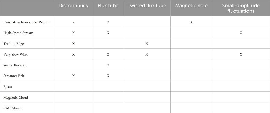
Table 1. The large-scale solar-wind structures in which small-scale structures were examined in this study; this table is not an indication of in which large-scale structures the small-scale structures can exist.

This paper is organized as follows. In Section 2 the data sets used for the study are discussed. Magnetic discontinuities are examined in Section 3, magnetic flux tubes are examined in Section 4, magnetic holes are examined in Section 5, and the ubiquitous small-amplitude magnetic-field fluctuations are examined in Section 6. The findings of this study are summarized in Section 7. Section 8 contains a discussion about the Fourier power (magnetic power spectral density) of the small-scale structures and the ubiquitous small-amplitude fluctuations outside of magnetic discontinuities.

2 The study

Two-spacecraft observations of small-scale magnetic structures in the solar wind are made with the THEMIS-B (THB) and the THEMIS-C (THC) spacecraft in lunar orbit, which are part of the ARTEMIS mission (Angelopoulos, 2011). This orbit is sketched in Figure 1 and the specific region of study is shaded in red. The nominal position of the Earth’s bow shock, as given by the Fairfield-Greenstadt model (Fairfield, 1971; Greenstadt et al., 1990), is drawn in blue. The region of study was chosen to minimize the effects of the foreshock, although bursts of large-amplitude quasi-periodic ion-foreshock waves (with periods ∼30 s) are occasionally seen in the THEMIS measurements (cf. Greenstadt et al., 1995; Salohub et al., 2022). The measurements used are from the FGM magnetic-field instrument (Auster et al., 2008) on THB and THC. The spatial separations between THB and THC are in the range of a few R_E (a few times 6,380 km). When needed, the solar-wind velocity is obtained from the THEMIS ESA instrument (McFadden et al., 2008) on THB and THC.

FGM data set was obtained using SPDF/CDAWeb; the “FGS” data set with ∼4-s time resolution for the magnetic-field vector measurements in GSE coordinates was downloaded. In the solar wind the THEMIS FGM data suffer from on-and-off systematic offsets between the B_z measurements on THB and the B_z measurements on THC. Also in the FGS data set, an hour or so before and an hour or so after an extended data dropout for one of the spacecraft, the FGM data from that spacecraft appear unreliable and are not utilized.

Magnetic-field structures are located by visually inspecting plots of the B_x, B_y, and B_z time-series from the two spacecraft. Plasma structures in the solar wind often accompany magnetic-field structures as characterized by the proton number density, the proton specific entropy, the ion composition, the electron temperature, and the intensity of the electron strahl (e.g., Borovsky, 2008, 2012; 2020a). However, in this report plasma structures are not investigated. A selection of magnetic-field structures in different types of large-scale solar-wind structures are displayed in the figures of this report (cf. Table 1).

3 Discontinuities

A solar-wind magnetic-field discontinuity is a rapid spatial jump in the properties of the solar-wind magnetic-field vector (it is a current sheet). With low-time-resolution temporal measurements the jumps appear “discontinuous” in the time series (e.g., Siscoe et al., 1968), but at higher time resolution the discontinuities are resolved and they are found to have various thicknesses (e.g., Vasquez et al., 2007). Discontinuities occur very frequently in the 1-AU time series, using 86-s time-averaged magnetic-field measurements from ACE, Borovsky (2008) identified 65,860 very strong (large-field-rotation) magnetic discontinuities in 7 years of solar-wind measurements, which is an average rate of 25.8 per day. Using higher-time-resolution magnetic-field data such as THEMIS finds a much-higher rate of occurrence because features like small-scale flux tubes, each with two discontinuities, are averaged away in 86-s data, so those flux tubes and their two discontinuties cannot be identified and counted.

Analysis of the heliospheric magnetic structure has focused on the question of whether current sheets (directional discontinuities) are tangential discontinuities (plasma boundaries) versus rotational discontinuities (propagating magnetic-field kinks) (e.g., Burlaga and Ness, 1969; Turner et al., 1971; Neugebauer, 1984; Lepping and Behannon, 1986; Soding et al., 2001). To determine whether a magnetic discontinuity is a rotational discontinuity versus a tangential discontinuity, the majority of studies focused on (1) determining the orientation of the current sheet, (2) determining the orientation of the local magnetic field, and then (3) using these two orientations to determine whether or not magnetic-field lines are crossing the discontinuity. Field lines crossing a current sheet indicates that it is a rotational discontinuity or that the current sheet is a “contact discontinuity” (Burlaga, 1971; Lapenta and Brackbill, 1996). Current sheets that do not have field lines crossing them are tangential discontinuities. Multispacecraft measurements indicate that current sheets are often highly oblique to the magnetic-field direction (Horbury et al., 2001; Knetter et al., 2003,2004; Riazantseva et al., 2005a) making this rotational-versus-tangential determination difficult (Neugebauer, 2006; Paschmann et al., 2013; Artemyev et al., 2019; Sonnerup, 2022). Looking for plasma-property jumps such as number-density jumps, proton-specific-entropy jumps, electron-temperature jumps, strahl-intensity jumps, ion-composition jumps, plasma-beta jumps, or magnetic-field-strength jumps across the discontinuity can confirm a discontinuity as being tangential (Borovsky, 2008; Riazantseva et al., 2005b; Borovsky, 2020a; Borovsky et al., 2021). Just as it is difficult to distinguish tangential versus rotational from the magnetic-field data because the normal-to-the-discontinuity field component is in general very small, it is difficult to distinguish tangential versus rotational from the plasma data, composition data, or strahl-intensity data because of noise in those data. Only larger changes can be clearly seen. This will be a problem into the future until more-specialized instrumentation is flown in the solar wind. In future, with higher-time-resolution and less-noisy particle measurements, more discontinuities could be confirmed as tangential (Borovsky and Raines, 2022). Rotational discontinuities theoretically have the property that they are “Alfvénic” and propagate through the solar-wind plasma at the Alfvén speed (Tsurutani and Ho, 1999; Neugebauer, 1984). As stated by Barnes (1971), tangential discontinuities are “stationary in the rest frame of the wind”. Note, however, that tangential discontinuities can be “Alfvenic” and propagate outward at a substantial fraction of the Alfvén speed relative to the proton solar wind speed. In the “Chandrasekhar dynamical equilibrium” model (Parker, 1979), all magnetic structure propagates outward from the Sun (in the Parker spiral direction) faster than the proton wind at a speed that is a fraction of the local Alfvén speed. If the tangled nonlinear magnetic-field sketched in Fig. 7.1 of Parker (1979) were drawn as a spaghetti of flux tubes separated by tangential discontinuities, then the discontinuities would propagate at a fraction of the local Alfvén speed even though they are everywhere strictly perpendicular to the local magnetic field (cf. Nemecek et al., 2020; Borovsky, 2020b).

In Figure 2 two examples of the THEMIS THB and THC spacecraft crossing discontinuities are shown. The data from THC is plotted in black with solid circles and the data from THB is plotted in gray with hollow circles. These two discontinuities are associated with distinct changes in the magnetic-field strength B_mag (cf. panels A and E) so they are both tangential discontinuities, even though the one in the second column is occurring in the Alfvénic fast solar wind of a coronal-hole origin. The discontinuity in the first column also shows a distinct jump in the plasma number density (not plotted). In Figure 2 the fact that B_mag changes means that the magnetic-field pressure (B_mag²/8π) changes, and so there must be a change in the plasma pressure to compensate this B_mag change. Hence, the two discontinuities in Figure 2 are co-located with plasma boundaries. The discontinuity in panels A–D was found in the trailing edge of a toward-magnetic-sector high-speed stream and the discontinuity in panels E–H was found in a toward-magnetic-sector high-speed stream. In the first column of Figure 2 there is about 40 s between the THC and THB observations of the discontinuity and in the second column the delay is about 20 s: these delays depend on (1) the relative positions of the two spacecraft, (2) the orientation of the discontinuity in the solar wind, and (3) the speed of the solar wind and the speed of the magnetic structure (cf. Borovsky, 2020b; Nemecek et al., 2020). In the first column of Figure 2 the discontinuity passes THC first (at 4.1 UT) and about 40 s later by THB (at 4.12 UT). The B_x profiles and B_y profiles appear quite similar between THB and THC, but in this case the B_z profiles differ. A B_z signature of the THC discontinuity can be seen, but no B_z signature is obvious for the discontinuity at THB.

Figure 2

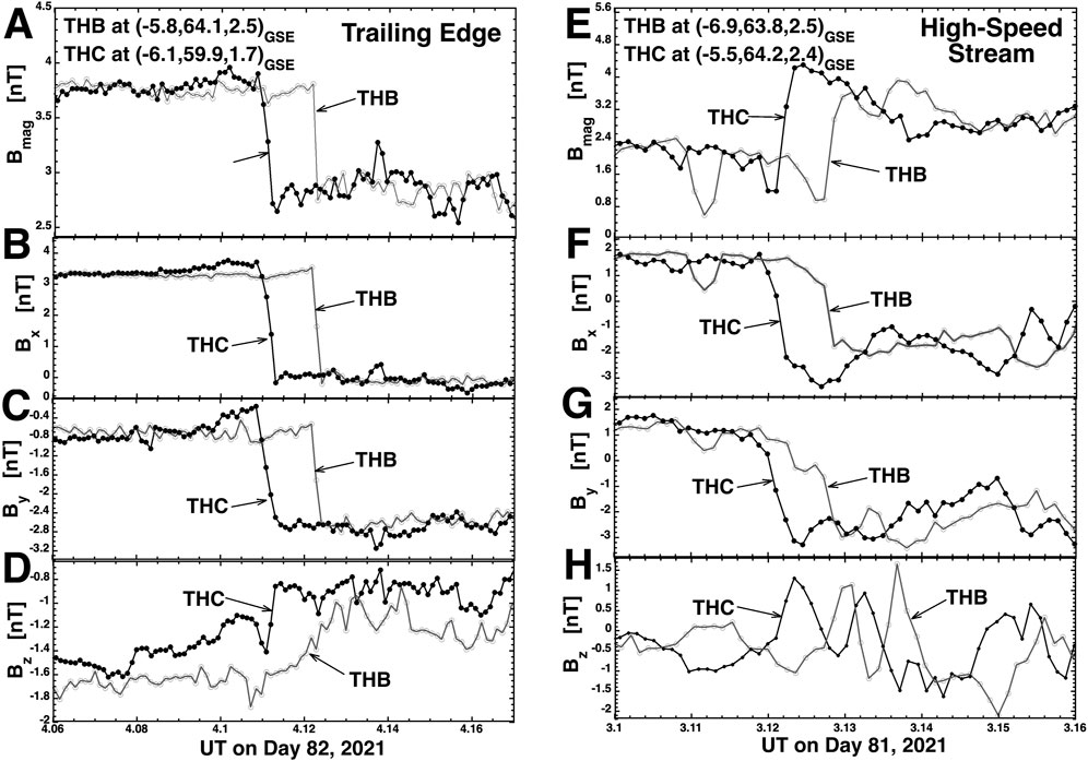
Figure 2. Examples of two discontinuities seen by THEMIS THB and THEMIS THC. Magnetic-field measurements from THB are plotted as the gray curve with hollow points and magnetic-field measurements from THB are plotted as the black curve with solid points. The labels of the figure are explained in the text of the paper.

In the second column of Figure 2 (panels E–H) this discontinuity is seen by THC at 3.12 UT and by THB at 3.13 UT. The B_x and B_y profiles of the discontinuity appear fairly similar between THB and THC. The discontinuity is difficult to clearly discern in B_z (panel H) since the B_z amplitude is weak, but signals can be seen at 3.12 UT and 3.13 UT.

In all of the panels of Figure 2 small-amplitude small-timescale magnetic-field fluctuations can be seen throughout the plots, typically with the small fluctuations seen by THB differing from the small fluctuations seen by THC.

Quite often discontinuities are observed that have different time-series profiles on THB and THC. Sometimes the temporal width of the magnetic-field change in the time series can differ, and sometimes the discontinuity can exhibit internal structure that is seen on one spacecraft but not seen on the other. In Figure 3 two discontinuities are examined wherein a sharp jump change is seen on one THEMIS spacecraft and a long ramp change is seen on the other nearby THEMIS spacecraft. In panels A–D THB observes a rapid jump and THC observes a slow ramp and in panels E–H THC observes a rapid jump and THB observes a slow ramp. The discontinuity of panels A–D was observed in a high-speed stream (toward magnetic sector) and the discontinuity of panels E–H was observed in a trailing edge. In panels A–D the jump has a width of about 8 s and the ramp has a width of about 48 s and in panels E–H the widths of the jump and of the ramp are about 8 s and about 72 s. The spatial widths that can be obtained from the temporal widths depend on the discontinuity orientation and the speed of the solar wind. In panels A–D of Figure 3 the Y-Z separation of THB and THC is δ_YZ = 3.3 R_E (1.7 × 10⁴ km) and in panels E–H the separation is δ_YZ = 4.8 R_E (2.5 × 10⁴ km). δ_YZ is the spacecraft separation perpendicular to the approximately X-direction flow of the solar wind. The inference is that the properties of discontinuities in the solar wind can vary over distances as small as a few R_E, where the thicknesses of discontinuities are typically less than 1 R_E (c.f. Vasquez et al., 2007).

Figure 3

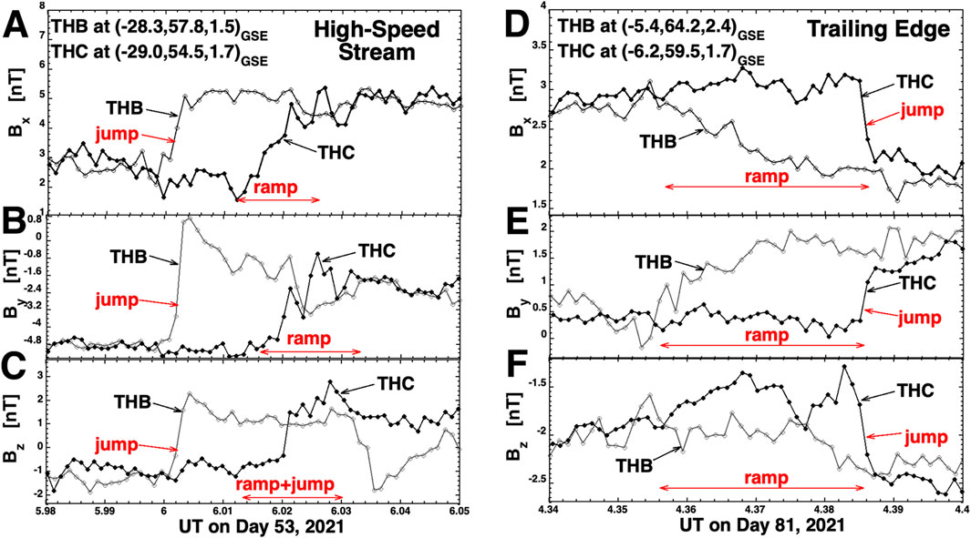
Figure 3. Examples of two magnetic flux tubes seen by THEMIS THB and THEMIS THC that have different morphologies as seen by the two spacecraft. Magnetic-field measurements from THB are plotted as the gray curve with hollow points and magnetic-field measurements from THB are plotted as the black curve with solid points. The labels of the figure are explained in the text of the paper.

With two-spacecraft observing the same discontinuity, it is possible to obtain information about the planarity (versus rippling or curvature) of the discontinuity. For 10 discontinuities in various types of large-scale solar-wind structures (cf. Table 2), such estimates are produced using FGM data from the THEMIS THB and THC spacecraft with variable separations for the 10 discontinuities. As each spacecraft passes through a discontinuity, the magnetic field rotates, hence the nomenclature “rotational discontinuity” or “directional discontinuity” (Burlaga, 1969; Vasquez and Hollweg, 2001). The cross-product method will be used to determine the local orientation of the plane of the discontinuity. When the normal to a discontinuity is perpendicular to the local magnetic field, the cross-product method is valid. When the normal to a discontinuity is nearly perpendicular to the local field, as measurements indicate they are (cf. Horbury et al., 2001; Knetter et al., 2003,2004; Neugebauer, 2006; Riazantseva et al., 2005a), then the cross-product method still works with an error in the normal direction of θ ∼ B_⊥/B_||, where B_⊥ is the component of the field perpendicular to the discontinuity and B_|| is the component of the field that is parallel to the plane of the discontinuity.

Table 2

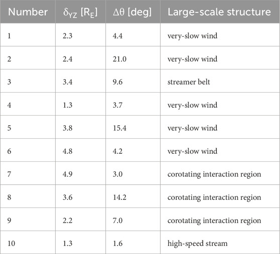
Table 2. Indications of the planarity of ten solar-wind discontinuities on R_E spatial scales.

Using the cross-product method as follows, the orientation of the normal to the local plane of the discontinuity is obtained from the time series measurements of the magnetic-field vector (e.g., Burlaga and Ness, 1969; Knetter et al., 2004; Borovsky, 2008). Comparing the direction of the normal to the discontinuity at the crossing location of one spacecraft with the direction of the normal at the crossing location of the other spacecraft, an indication of the flatness of the discontinuity is obtained. Here the magnetic-field direction B_enter as the spacecraft enters the discontinuity is used with the field direction B_exit as the spacecraft exits to obtain the cross product C = B_enter × B_exit, which is normalized to c, where the direction of c is the direction of the local normal. The comparison between the two spacecraft crossings is done via the dot product c₁•c₂, where Δθ = arccos (c₁•c₂) is the angular difference between the two normal vectors: if the discontinuity is perfectly planar then Δθ = 0^o. Errors in this technique come mainly from (1) small-scale magnetic-field fluctuations throughout the solar wind, (2) systematic offsets between the B_z values in the THB and THC data sets, and (3) measurement noise in the magnetometer data set. The mean magnetic-field strength for the 10 discontinuities of Table 2 is 5.0 nT. If the measurement noise level is 0.05 nT, then the approximate error in the direction of the local discontinuity normal is θ ∼ 2 (0.05 nT)/(5.0 nT) = 1.2^o. This measurement-noise error is smaller than the error caused by the presence of small-scale magnetic-field fluctuations. For the discontinuity analysis of Table 2, times when the B_z offsets were small were used. Table 2 finds a number of small values for Δθ for the 10 discontinuities and it also finds some larger values. Spacecraft separations δ_YZ in the Y versus Z positions of THB and THC are listed in the table. For comparison, if flux tubes have a typical diameter of 60 R_E (cf. Borovsky, 2008) and they are cylindrical, then a change Δθ of ≤1.9^o is expected for every 1 R_E of δ_YZ: eight of the 10 values of Δθ in Table 2 exceed this expectation. Note, however, that the flux tubes are likely to be more like a two-dimensional foam (soap bubbles) (Weaire and Hutzler, 1999) or a Voronoi tessellation (Mahin et al., 1980; Okabe et al., 2000) with a large fraction of their boundary areas to be flat and with flat regions with different orientations connected by a vertex. For the data of Table 2, no significant correlation is found between Δθ and δ_YZ. The low values of Δθ in Table 2 indicate that these discontinuities are quasi-planar over the scale of δ_YZ. The high values of Δθ in Table 2 indicate either (1) that the discontinuity is not planar on the scale of δ_YZ6, (2) the two spacecraft cross on two sides of a vertex, or (3) that the planarity test failed (perhaps owing to the presence of small-scale magnetic-field fluctuations).

4 Flux tubes

Flux tubes in the solar wind are distinct bundles of magnetic-field lines, often bounded by discontinuities. Within a typical flux tube the magnetic field is quasi uniform, with small-amplitude small-scale magnetic-field fluctuations. The axial orientation of the flux tube is taken to be the orientation of the magnetic-field vector within the tube. Flux tubes can exhibit distinct plasma properties (such as the proton number density, proton specific entropy, ion composition, and electron temperature) and distinct values of the intensity of the electron strahl (e.g., Borovsky, 2008, 2012; 2020a), but only the magnetic-field properties of the flux tubes are investigated here.

In panels A–D of Figure 4 THB enters and exits a flux tube at about 0.24 UT and 0.29 UT with THC following THB by about 12 s–20 s. This flux tube is about 2.7-min in duration in the time series with a solar-wind speed of about 359 km/s. In panels E–H THB enters and exits the flux tube at about 19.35 UT and 19.44 UT with THC following by about 12 s. This flux tube is about 5.9-min in duration in the time series with a solar-wind speed of about 643 km/s.

Figure 4

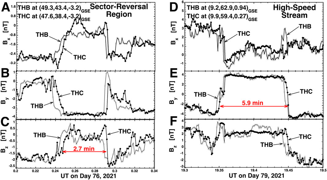
Figure 4. Examples of two small flux tubes seen by THEMIS THB and THEMIS THC. Magnetic-field measurements from THB are plotted as the gray curve with hollow points and magnetic-field measurements from THB are plotted as the black curve with solid points. The labels of the figure are explained in the text of the paper.

In the two cases of Figure 4 the profiles of the leading and trailing boundaries of the flux tubes appear very similar in THB and THC: this is often not the case for solar-wind magnetic flux tubes. The flux tube observed in panels A–D of Figure 5 is bounded on the leading edge by a sharp discontinuity with a temporal width of 12 s and on the trailing edge by a slow ramp with a temporal width of 126 s. The discontinuity and ramp are clearly seen in B_y (panel C) and B_z (panel D), and faintly seen in B_x (panel B). Note in panel A the magnetic-hole-like decrease of B_mag during the ramp phase at the trailing edge of the flux tube: Burlaga (1968) suggests that this is a sign of magnetic-field annihilation.

Figure 5

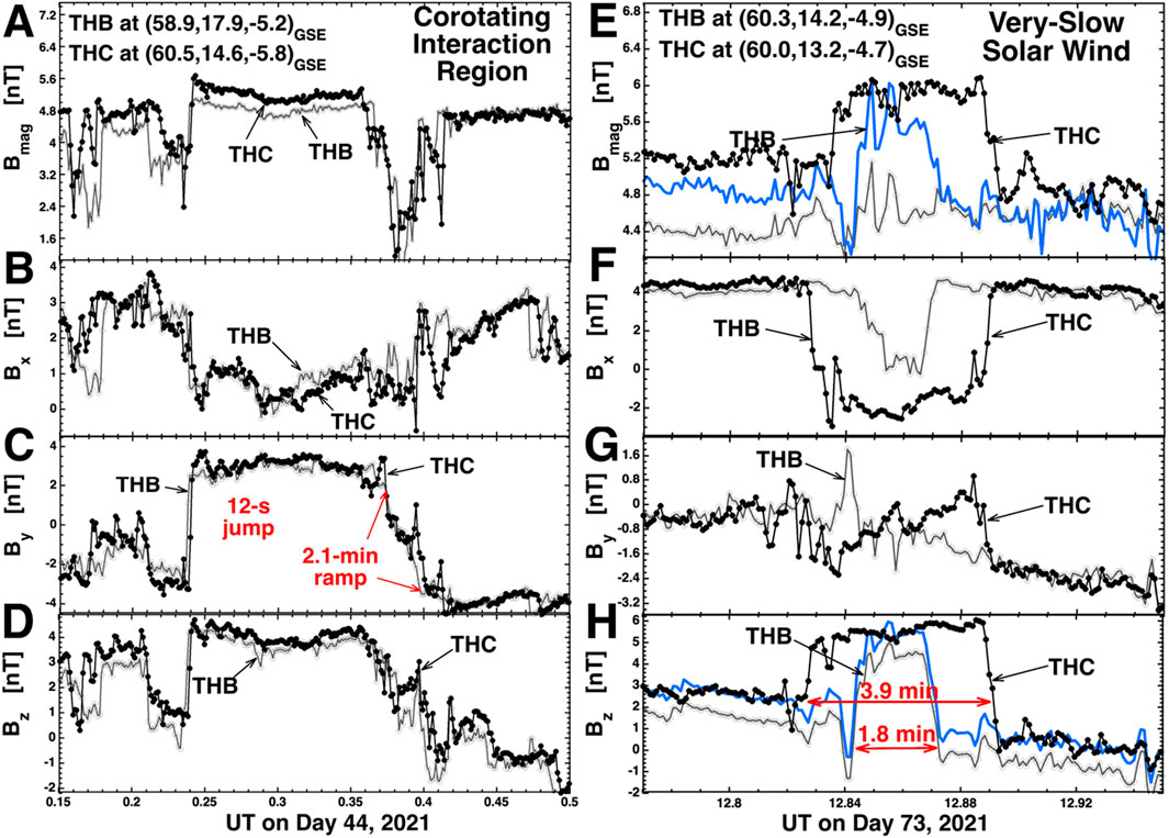
Figure 5. Examples of two magnetic flux tubes seen by THEMIS THB and THEMIS THC. In panels (A–D) the flux tube exhibits different morphologies for its leading and trailing boundaries. In panels (E–H) THB and THC see the flux tube with differing time durations. The blue curves in panels E and H are attempts to correct for the Bz offsets between the THB and THC data. Magnetic-field measurements from THB are plotted as the gray curve with hollow points and magnetic-field measurements from THB are plotted as the black curve with solid points.

Panels E–H of Figure 5 shows an example where a flux tube is seen with different sizes on the two different THEMIS spacecraft. Here THC observes the flux tube with a temporal size of about 3.9 min in its FGM time series while THB observes a 1.8-min flux tube. The most likely cause for this observed difference is a difference in where the two spacecraft cross through the flux tube, with THC crossing closer to the center of the tube and THB crossing closer to the edge of the tube. Panels E–H might yield the conclusion that the flux tube has a variable diameter going along the flux-tube axis. But if this were so, then magnetic-flux conservation would say that B_mag must be substantially higher in the smaller portion of the tube than in the larger portion of the tube. In panel E of Figure 5 the magnetic-field strength is plotted. The black solid-point curve is from THC and the gray hollow-point curve is from THB. Note in panel H that there is a systematic offset between B_z on THB versus THC, with B_z of THB being about 1 nT lower than B_z of THC. This offset is approximately corrected by adding 1 nT to B_z of THB, and this correction is plotted in panel H as the blue line. Using this “corrected” THB B_z to calculate B_mag of THB results in the blue curve in panel E. The blue curve of panel E indicates that B_mag within the smaller flux tube as seen by THB is not substantially larger than B_mag of the larger flux tube as seen by THC. Hence, panels E–H of Figure 5 are not consistent with a change in the diameter of the flux tube with distance along the tube.

Most solar-wind flux tubes have uniform magnetic-field vectors inside of them (cf. Figure 4), but some tubes exhibit a magnetic twist wherein one or more of the magnetic-field components exhibits a slow variation across the flux tube. Some of these twisted flux tubes may be flux ropes (Moldwin et al., 2000; Feng et al., 2008).

Two examples of twisted flux tubes are exhibited in Figure 6: A small tube (83-s in duration) in panels A–D and a larger tube (11.2-min in duration) in panels E–H. The flux tube in panels A–D has a dominant B_y component with all three field components changing smoothly (but with small-scale noise) across the tube: hence one envisions a tube aligned in the Y direction with a twisted magnetic field inside the tube. Panel A shows that the magnetic-field strength B_mag is weaker inside the tube than it is outside the tube. Note the advection lag between the two THEMIS spacecraft with THC observing the flux tube first.

Figure 6

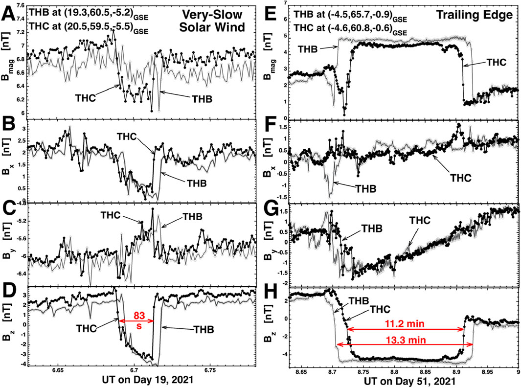
Figure 6. Examples of two twisted small flux tubes seen by THEMIS THB and THEMIS THC. Magnetic-field measurements from THB are plotted as the gray curve with hollow points and magnetic-field measurements from THB are plotted as the black curve with solid points. The labels of the figure are explained in the text of the paper.

The larger tube in panels E–H of Figure 6 has a uniform B_z component with B_x and By changing smoothly across the tube. This envisions a flux tube aligned in the Z direction with a magnetic twist. Panel E shows that the flux tube has a stronger value of B_mag than does the surrounding plasma. Note that this flux tube is seen with different sizes by THB versus THC: this is probably a function of where the two spacecraft paths cut through the tube. Note in panel E the magnetic-hole-like structure (strongly reduced values of B_mag) on the leading edge of this twisted tube: note again the Burlaga (1968) suggestion of magnetic-field annihilation.

In Figure 7 two flux tubes that are displayed that are seen by only a single THEMIS spacecraft: in both cases THB observes the flux tube while THC does not. The flux tube of panels A–C was found in a high-speed stream and the flux tube of panels D–F was found in slow wind (streamer belt). Both flux tubes have dominant B_z fields inside. As viewed from the Sun the flux tube of panels A–C is tilted arctan (B_y/B_z) = arctan (1.2 nT/2.4 nT) = 27^o away from the Z direction and the flux tube of panels D–F is tilted arctan (B_y/B_z) = arctan (0.8 nT/3.5 nT) = 13^o away from the Z direction as viewed from the Sun. The distance between THEMIS THB and THC in the Y direction is 4.9 R_E = 3.1 × 10⁴ km in panels A–C and it is 2.3 R_E = 1.5 × 10⁴ km in panels D–F. As a flux tube advects in the X direction with the solar wind and has a finite diameter, it is conceivable that the flux tube hits one spacecraft and misses the other. The 5.8-min size of the flux tube as seen by THB in panel C along with a solar-wind speed of 632 km/s yields a size of 34.6 R_E = 2.2 × 10⁵ km where THB cuts through the tube and the 2.2-min duration of the flux tube seen by THB in panel F along with a solar-wind speed of 297 km/s yields a size estimate of 6.2 R_E = 3.9 × 10⁴ km. This missing scenario is more probable for the smaller flux tube of panels D–F.

Figure 7

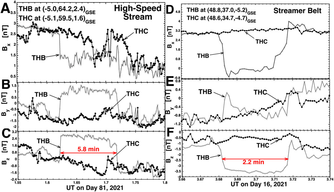
Figure 7. Examples of two discontinuities that are seen by only one of the THEMIS THB and THEMIS THC spacecraft. Magnetic-field measurements from THB are plotted as the gray curve with hollow points and magnetic-field measurements from THB are plotted as the black curve with solid points. The labels of the figure are explained in the text of the paper.

5 Magnetic holes

Magnetic holes in the solar wind are spatially localized reductions of the magnetic-field-strength B_mag (Turner et al., 1977; Winterhalter et al., 1994, 2000; Roytershteyn et al., 2015; Yu et al., 2021). Two small-scale magnetic holes are examined in Figure 8, one (panels A–D) is 18.5 s in duration as seen by THEMIS THC and the other (panels E–H) is 9.4 s in duration as seen by THEMIS THB. Both were observed in a corotating interaction region of the solar wind. Each of the two magnetic holes is only observed by one spacecraft. The magnetic holes are clearly seen in the time-series plots of B_mag in panels A and E. In panel A B_mag goes from about 6.8 nT to about 0.9 nT and in plot E B_mag goes from 6.3 nT to 1.5 nT. Strong signatures of these two magnetic holes are also seen in B_x (panels B and F) and in B_y (panels C and G). For these two magnetic holes, signatures are not clear in B_z (panels D and H). Note that the direction of the magnetic field changes within these two magnetic holes.

Figure 8

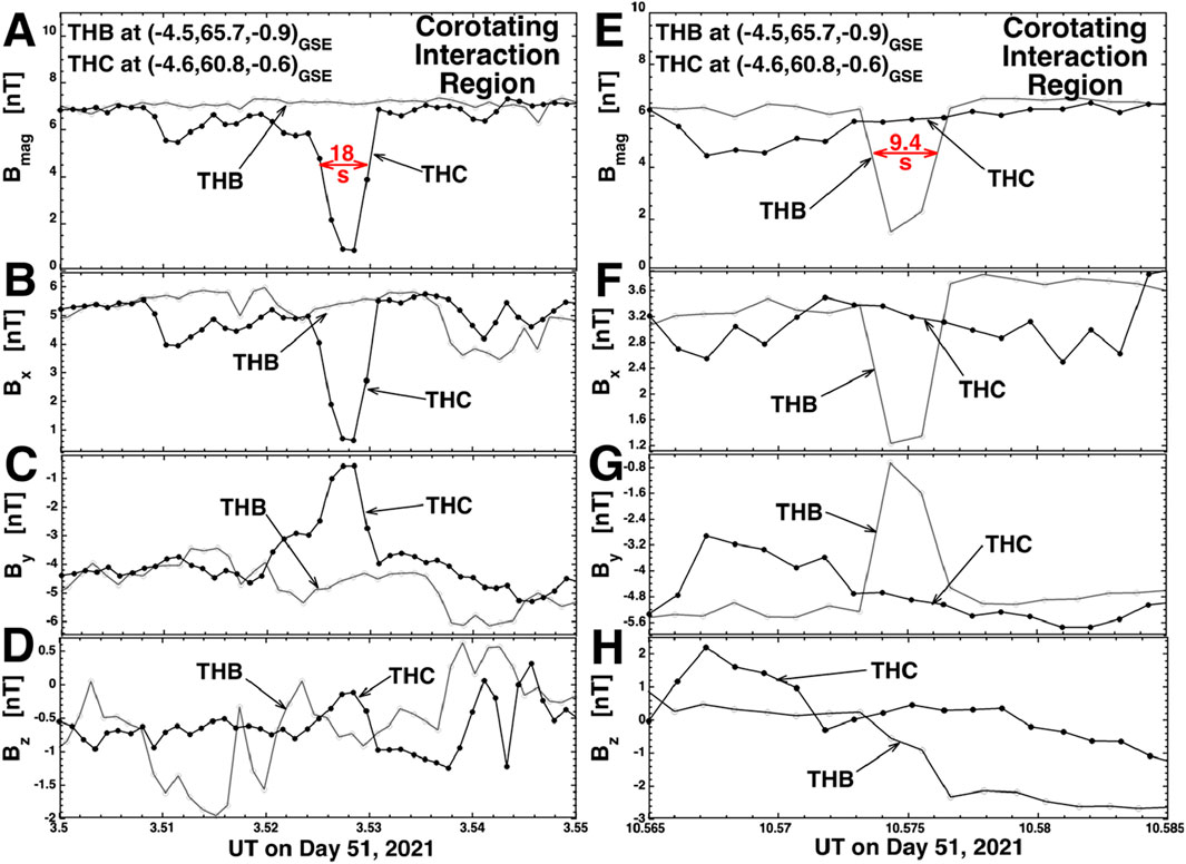
Figure 8. Examples of two small magnetic holes seen by THEMIS THB and THEMIS THC. In each example, only one spacecraft observes the magnetic hole. Magnetic-field measurements from THB are plotted as the gray curve with hollow points and magnetic-field measurements from THB are plotted as the black curve with solid points. The labels of the figure are explained in the text of the paper.

Looking at panel A of Figure 8, with a duration of 18 s and a wind speed of 473 km/s the spatial size of the portion of the magnetic hole penetrated by THC is 1.3 R_E = 8500 km, while the Y separation between THB and THC is 4.9 R_E. Hence, it is quite plausible that this small magnetic hole can hit THC but miss THB. Looking at panel E, with a duration of 9.4 s and a wind speed of 529 km/s the spatial size of the portion of the magnetic hole penetrated by THB is 0.8 R_E = 5000 km, while the Y separation between THB and THC is 4.5 R_E. Hence, it is also quite plausible that this small magnetic hole can hit THB but miss THC.

6 Ubiquitous small-amplitude magnetic-field fluctuations

Small-amplitude small-scale magnetic-field fluctuations seem “ubiquitous” in the solar wind at 1 AU; they are observed outside of the large-amplitude magnetic-field structures and inside of the large-amplitude magnetic-field structures (for example, the inside of the flux tubes in Figure 4). In this study with THB and THC the investigator inspected high-time-resolution plots of the B_x, B_y, and B_z time-series data whenever the THEMIS spacecraft were in the “range of study” depicted in red in Figure 1. At no time did the investigator observe time intervals when there were not low-amplitude magnetic fluctuations. Magnetic clouds are defined by a “smooth” rotation of the magnetic field (e.g., Gosling et al., 1987; Burlaga et al., 1998), yet fluctuations can be detected and analyzed even within magnetic clouds (Smith et al., 2006; Andreeova et al., 2013; Zubair et al., 2023). Sometimes the small-amplitude fluctuations observed by THB seem completely independent of the small-amplitude fluctuations seen by THC; at other times with similar spacecraft separation distances both THEMIS spacecraft observe the same fluctuations. The origin, evolution, lifetime, and physical nature of these small-scale magnetic-field fluctuations is not known.

A case where the small-amplitude fluctuations appear completely different on THB versus THC is shown in panels A–C of Figure 9. This is an interval of FGM measurements in a high-speed stream (toward magnetic sector). The magnetic-field components measured by THC are plotted in black and the components measured by THB are plotted in red. Even with time shifting one time series relative to the other to account for propagation times, the fluctuations in the two time series are different for B_x, B_y, and B_z. This indicates that for this event the small-amplitude magnetic-field fluctuations have spatial scales transverse to the solar-wind flow that are smaller than the spacecraft separations.

Figure 9

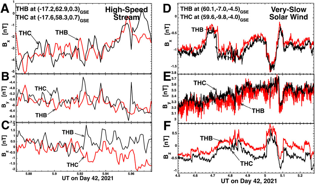
Figure 9. Two examples of the ubiquitous small-amplitude magnetic-field fluctuations seen by THEMIS THB and THEMIS THC. In panels (A–C) the fluctuations as observed by THB and THC are independent and in panels (D–F) the fluctuations as observed by THB and THC are highly correlated. Magnetic-field measurements from THB are plotted as the red curve and magnetic-field measurements from THB are plotted as the black curve.

A case where the small-amplitude magnetic-field fluctuations appear the same on THB and on THC is shown in panels D–F of Figure 9. This is an interval of FGM measurements in very slow solar wind. For all three magnetic-field components the magnetic-field changes observed by THB are see also by THC. (Note in panel F the systematic offset of B_z between THB and THC.) This indicates that the small-amplitude fluctuations for this event have spatial scales larger than the spacecraft separations.

These ubiquitous small-amplitude magnetic-field fluctuations are an integral part of the structure and physics of the solar wind. In future a two-spacecraft statistical study of the small-amplitude magnetic-field fluctuations of the solar wind is warranted to determine when and where they are independent on the two spacecraft and when and where they are the same.

7 Findings

This study examined small-scale magnetic-field structures in the solar wind using measurements at 1 AU from the two THEMIS spacecraft THB and THC in lunar orbit with their unique spacecraft spatial separations of ∼1 R_E to a few R_E. Small-scale magnetic-field structures are separated into four types: discontinuities (current sheets), magnetic flux tubes, magnetic holes, and small-amplitude magnetic-field fluctuations. The findings in this study are the following.

1 The properties of solar-wind discontinuities can vary substantially over distances as small as a few R_E: those few-R_E distances are only a few times thicknesses of the discontinuities.

2 In two-spacecraft tests to gauge the planarity of solar-wind discontinuities, sometimes the discontinuities appear flat on spatial scales of a few R_E and sometimes flatness is not found. When flatness is not found, it could be that the test has failed owing to small-amplitude magnetic-field fluctuations.

3 Magnetic flux tubes are most-easily discerned in the magnetic-field time series measurements when the tubes are bounded by discontinuities. However, flux tubes that are bounded on one side by a discontinuity and on the other side by a broad magnetic ramp are also found.

4 As would be expected for small structures, small flux tubes were sometimes observed on only one of the THEMIS spacecraft when the spacecraft separations were a few R_E.

5 Again, as would be expected for small structures, magnetic holes were sometimes observed on only one of the THEMIS spacecraft when the spacecraft separations were a few R_E.

6 In the THEMIS THB and THC FGM data sets (with spacecraft separations of a few R_E), the ubiquitous small-amplitude magnetic-field fluctuations in the solar wind sometimes appear to be the same at THB and THC and sometimes the fluctuations appear to be completely independent at the two spacecraft positions. The small-amplitude fluctuations appear everywhere, even inside of the small-scale structures such as flux tubes.

Future statistical studies of the various types of solar-wind small-scale magnetic structures are very warranted, particularly if improved instrumentation should come into fruition.

8 Discussion: small-scale structures and the magnetic power spectrum of the solar wind

In a series of papers it has been demonstrated (1) that the amplitude and slope of the solar-wind inertial-range magnetic power-spaectal-density spectrum is determined by the amplitude and occurrence rate of discontinuities (Siscoe et al., 1968; Borovsky, 2010), (2) that the frequency of the spectral breakpoint at the high-frequency end of the inertial range is determined by the thicknesses of discontinuities (Borovsky and Podesta, 2015; Podesta and Borovsky, 2016), and (3) that the spectral slope at frequencies above that breakpoint is influenced by the internal profiles of the discontinuities (Borovsky and Burkholder, 2020). The narrow discontinuities contain Fourier power at all frequencies, much like the Fourier transform of a step function. The Fourier transform of flux tubes or magnetic holes will reflect the properties of the discontinuity boundaries.

It would be very interesting, and it will be the topic of a future study, to examine the Fourier properties of the ubiquitous small-amplitude magnetic-field fluctuations between the discontinuities. Bruno et al. (2001) suggested that the smaller fluctuations between the discontinuities (i.e., inside the flux tubes) are the real turbulent fluctuations of the solar wind. Perhaps they are instability-induced fluctuations (e.g., Bale et al., 2009; Navarro et al., 2014). To properly do this Fourier study multiple intervals of small-amplitude-fluctuation data must be strung together into a larger time series, and to avoid artificial discontinuities in the time series at the boundaries between intervals Gaussian windowing must be used at the boundaries of the intervals. Although the structures of interest are from relatively short time series, more advanced techniques such as Detrended Fluctuations Analysis in the field of space physics (e.g., Veronese et al., 2011) could be applied in future work to more finely study the fluctuation patterns arising from the comprehensive complexity of the solar wind.

Data availability statement

Publicly available datasets were analyzed in this study. This data can be found here: All data used in this study are available at the NASA SPDF/CDAWeb server at https://cdaweb.gsfc.nasa.gov.

Author contributions

JB: Methodology, Conceptualization, Writing – review and editing, Funding acquisition, Writing – original draft, Formal Analysis, Visualization.

Funding

The author(s) declare that financial support was received for the research and/or publication of this article. At the Space Science Institute by the NASA HERMES Interdisciplinary Science Program via grant 80NSSC21K1406, by the NSF Magnetospheric Program via grant AGS-2149822, and by the NASA LWS Program via grant 80NSSC23.

Acknowledgments

The author thanks Vassilis Angelopoulos for helpful conversations.

Conflict of interest

The author declares that the research was conducted in the absence of any commercial or financial relationships that could be construed as a potential conflict of interest.

The author(s) declared that they were an editorial board member of Frontiers, at the time of submission. This had no impact on the peer review process and the final decision.

Generative AI statement

The author(s) declare that no Generative AI was used in the creation of this manuscript.

Any alternative text (alt text) provided alongside figures in this article has been generated by Frontiers with the support of artificial intelligence and reasonable efforts have been made to ensure accuracy, including review by the authors wherever possible. If you identify any issues, please contact us.

Publisher’s note

All claims expressed in this article are solely those of the authors and do not necessarily represent those of their affiliated organizations, or those of the publisher, the editors and the reviewers. Any product that may be evaluated in this article, or claim that may be made by its manufacturer, is not guaranteed or endorsed by the publisher.

References

Angelopoulos, V. (2011). The ARTEMIS mission. Space Sci. Rev. 165, 3–25. doi:10.1007/s11214-010-9687-2

CrossRef Full Text | Google Scholar

Artemyev, A. V., Angelopoulos, V., and Vasko, I. Y. (2019). Kinetic properties of solar wind discontinuities at 1 AU observed by ARTEMIS. J. Geophys. Res. Space Phys. 124, 3858–3870. doi:10.1029/2019ja026597

CrossRef Full Text | Google Scholar

Auster, A. U., Glassmeier, K. H., Magnes, W., Aydogar, O., Baumjohann, W., Constantinescu, D., et al. (2008). The THEMIS fluxgate magnetometer. Space Sci. Rev. 141, 235–264. doi:10.1007/s11214-008-9365-9

CrossRef Full Text | Google Scholar

Bale, S. D., Kasper, J. C., Howes, G. G., Quataert, E., Salem, C., and Sundkvist, D. (2009). Magnetic fluctuation power near proton temperature anisotropy instability thresholds in the solar wind. Phys. Rev. Lett. 103, 211101. doi:10.1103/PhysRevLett.103.211101

PubMed Abstract | CrossRef Full Text | Google Scholar

Barnes, A. (1971). Theoretical constraints on the microscale fluctuations in the interplanetary medium. J. Geophys. Res. 76, 7522–7526. doi:10.1029/ja076i031p07522

CrossRef Full Text | Google Scholar

Bartley, W. C., Bukata, R. P., McCracken, K. G., and Rao, U. R. (1966). Anisotropic cosmic radiation fluxes of solar origin. J. Geophys. Res. 71, 3297–3304. doi:10.1029/jz071i013p03297

CrossRef Full Text | Google Scholar

Borovsky, J. E. (2008). The flux-tube texture of the solar wind: strands of the magnetic carpet at 1 AU? J. Geophys. Res. 113, A08110. doi:10.1029/2007JA012684

CrossRef Full Text | Google Scholar

Borovsky, J. E. (2010). Contribution of strong discontinuities to the power spectrum of the solar wind. Phys. Rev. Lett. 105, 111102. doi:10.1103/PhysRevLett.105.111102

PubMed Abstract | CrossRef Full Text | Google Scholar

Borovsky, J. E. (2012). Looking for evidence of mixing in the solar wind from 0.31 to 0.98 AU. J. Geophys. Res. 117, A06107. doi:10.1029/2012JA017525

CrossRef Full Text | Google Scholar

Borovsky, J. E. (2020a). The magnetic structure of the solar wind: ionic composition and the electron strahl. Geophys. Res. Lett. 47, e2019GL084586. doi:10.1029/2019GL084586

CrossRef Full Text | Google Scholar

Borovsky, J. E. (2020b). On the motion of the heliospheric magnetic structure through the solar wind plasma. J. Geophys. Res. 125, e2019JA027377. doi:10.1029/2019JA027377

CrossRef Full Text | Google Scholar

Borovsky, J. E., and Burkholder, B. L. (2020). On the Fourier contribution of strong current sheets to the high-frequency magnetic power spectral density of the solar wind. J. Geophys. Res. Space Phys. 125, e2019JA027307. doi:10.1029/2019JA027307

CrossRef Full Text | Google Scholar

Borovsky, J. E., and Denton, M. H. (2016). The trailing edges of high-speed streams at 1 AU. J. Geophys. Res. 121, 6107–6140. doi:10.1002/2016JA022863

CrossRef Full Text | Google Scholar

Borovsky, J. E., and Podesta, J. J. (2015). Exploring the effect of current sheet thickness on the high-frequency Fourier spectrum breakpoint of the solar wind. J. Geophys. Res. 120, 9256–9268. doi:10.1002/2015JA021622

CrossRef Full Text | Google Scholar

Borovsky, J. E., and Raines, J. M. (2022). Heliospheric Structure Analyzer (HSA): a simple 1-AU Mission concept focusing on Large-Geometric- factor measurements. Front. Astron. Space Sci. 9, 919755. doi:10.3389/fspas.2022.919755

CrossRef Full Text | Google Scholar

Borovsky, J. E., Halekas, J. S., and Whittlesey, P. L. (2021). The electron structure of the solar wind. Front. Astron. Space Sci. 8, 690005. doi:10.3389/fspas.2021.690005

CrossRef Full Text | Google Scholar

Bruno, R. (2019). Intermittency in solar wind turbulence from fluid to kinetic scales. Earth Space Sci. 6, 656–672. doi:10.1029/2018EA000535

CrossRef Full Text | Google Scholar

Bruno, R., Carbone, V., Veltri, P., Pietropaolo, E., and Bavassano, B. (2001). Identifying intermittency events in the solar wind. Planet. Space Sci. 49, 1201–1210. doi:10.1016/s0032-0633(01)00061-7

CrossRef Full Text | Google Scholar

Burlaga, L. F. (1968). Micro-scale structures in the interplanetary medium. Sol. Phys. 4, 67–92. doi:10.1007/BF00146999

CrossRef Full Text | Google Scholar

Burlaga, L. F. (1969). Directional discontinuities in the interplanetary magnetic field. Sol. Phys. 7, 54–71. doi:10.1007/BF00148406

CrossRef Full Text | Google Scholar

Burlaga, L. F. (1971). Hydromagnetic waves and discontinuities in the solar wind. Space Sci. Rev. 12, 600–657. doi:10.1007/bf00173345

CrossRef Full Text | Google Scholar

Burlaga, L. F., and Ness, N. F. (1969). Tangential discontinuities in the solar wind. Sol. Phys. 9, 467–477. doi:10.1007/BF02391672

CrossRef Full Text | Google Scholar

Burlaga, L., Fitzenreiter, R., Lepping, R., Ogilvie, K., Szabo, A., Lazarus, A., et al. (1998). A magnetic cloud containing prominence material: january 1997. J. Geophys. Res. 103, 277–285. doi:10.1029/97ja02768

CrossRef Full Text | Google Scholar

Fairfield, D. H. (1971). Average and unusual locations of the Earth’s magnetopause and bow shock. J. Geophys. Res. 28, 6700–6716. doi:10.1029/ja076i028p06700

CrossRef Full Text | Google Scholar

Feng, H. Q., Wu, D. J., Lin, C. C., Chao, J. K., Lee, L. C., and Lyu, L. H. (2008). Interplanetary small- and intermediate-sized magnetic flux ropes during 1995–2005. J. Geophys. Res. 113, A12105. doi:10.1029/2008JA013103

CrossRef Full Text | Google Scholar

Gosling, J. T., Asbridge, J. R., Bame, S. J., and Feldman, W. C. (1978). Solar wind stream interfaces. J. Geophys. Res. 83, 1401–1412. doi:10.1029/JA083iA04p01401

CrossRef Full Text | Google Scholar

Gosling, J. T., Baker, D. N., Bame, S. J., Feldman, W. C., Zwickl, R. D., and Smith, E. J. (1987). Bidirectional solar Wind Electron heat flux events. J. Geophys. Res. 92, 8519–8535. doi:10.1029/ja092ia08p08519

CrossRef Full Text | Google Scholar

Greco, A., Chuychai, P., Matthaeus, W. H., Servidio, S., and Dmitruk, P. (2008). Intermittent MHD structures and classical discontinuities. Geophys. Res. Lett. 35, L19111. doi:10.1029/2008gl035454

CrossRef Full Text | Google Scholar

Greco, A., Perri, S., Servidio, S., Yordanova, E., and Veltri, P. (2016). The complex structure of magnetic field discontinuities in the turbulent solar wind. ApJ 823, L39. doi:10.3847/2041-8205/823/2/l39

CrossRef Full Text | Google Scholar

Greenstadt, E. W., Traver, D. P., Coroniti, F. V., Smith, E. J., and Slavin, J. A. (1990). Observations of the flank of the Earth’s bow shock to -110 R_E by ISEE 3/ICE. Geophys. Res. Lett. 17, 753–756. doi:10.1029/GL017i006p00753

CrossRef Full Text | Google Scholar

Greenstadt, E. W., Le, G., and Strangeway, R. J. (1995). ULF waves in the foreshock. Adv. Space Res. 15 (8-9), 71–84. doi:10.1016/0273-1177(94)00087-H

PubMed Abstract | CrossRef Full Text | Google Scholar

Horbury, T. S., Burgess, D., Fränz, M., and Owen, C. J. (2001). Three spacecraft observations of solar wind discontinuities. Geophys. Res. Lett. 28, 677–680. doi:10.1029/2000gl000121

CrossRef Full Text | Google Scholar

Knetter, T., Neubauer, F. M., Horbury, T., and Balogh, A. (2003). Discontinuity observations with Cluster. Adv. Space Res. 32 (4), 543–548. doi:10.1016/s0273-1177(03)00335-1

CrossRef Full Text | Google Scholar

Knetter, T., Neubauer, F. M., Horbury, T., and Balogh, A. (2004). Four-point discontinuity observations using Cluster magnetic field data: a statistical survey. J. Geophys. Res. 109, A06102. doi:10.1029/2003JA010099

CrossRef Full Text | Google Scholar

Lapenta, G., and Brackbill, J. U. (1996). Contact discontinuities in collisionless plasmas: A comparison of hybrid and kinetic simulations. Geophys. Res. Lett. 23, 1713. doi:10.1029/96GL01845

CrossRef Full Text | Google Scholar

Lepping, R. P., and Behannon, K. W. (1986). Magnetic field directional discontinuities characteristics between 0.46 and 1 AU. J. Geophys. Res. 91, 8725. doi:10.1029/JA091iA08p08725

CrossRef Full Text | Google Scholar

Mahin, K. W., Hanson, K., and Morris, J. W. (1980). Comparative analysis of the cellular and Johnson-Mehl microstructures through computer simulation. Acta Metall. 28, 443–453. doi:10.1016/0001-6160(80)90134-0

CrossRef Full Text | Google Scholar

McCracken, K. G., and Ness, N. F. (1966). The collimation of cosmic rays by the interplanetary magnetic field. J. Geophys. Res. 71, 3315–3318. doi:10.1029/jz071i013p03315

CrossRef Full Text | Google Scholar

McFadden, J. P., Carlson, C. W., Larson, D., Ludlam, M., Abiad, R., Elliott, B., et al. (2008). The THEMIS ESA plasma instrument and in-flight calibration. Space Sci. Rev. 141, 277–302. doi:10.1007/s11214-008-9440-2

CrossRef Full Text | Google Scholar

Michel, F. C. (1967). Model of solar wind structure. J. Geophys. Res. 72, 1917–1932. doi:10.1029/jz072i007p01917

CrossRef Full Text | Google Scholar

Moldwin, M. B., Ford, S., Lepping, R., Slavin, J., and Szabo, A. (2000). Small-scale magnetic flux ropes in the solar wind. Geophys. Res. Lett. 27, 57–60. doi:10.1029/1999GL010724

CrossRef Full Text | Google Scholar

Navarro, R. E., Moya, P. S., Muñoz, V., Araneda, J. A., Viñas, A. F., and Valdivia, J. A. (2014). Solar wind thermally induced magnetic fluctuations. Phys. Rev. Lett. 112, 245001. doi:10.1103/PhysRevLett.112.245001

PubMed Abstract | CrossRef Full Text | Google Scholar

Nemecek, Z., Durovcova, T., Safrankova, J., Nemec, F., Matteini, L., Stansby, D., et al. (2020). What is the solar wind frame of reference? Astrophys. J. 889, 163. doi:10.3847/1538-4357/ab65f7

CrossRef Full Text | Google Scholar

Neugebauer, M. (2006). Comment on the abundances of rotational and tangential discontinuities in the solar wind. J. Geophys. Res. 111, A04103. doi:10.1029/2005ja011497

CrossRef Full Text | Google Scholar

Neugebauer, M., and Giacalone, J. (2015). Energetic particles, tangential discontinuities, and solar flux tubes. J. Geophys. Res. Space Phys. 120, 8281–8287. doi:10.1002/2015ja021632

CrossRef Full Text | Google Scholar

Neugebauer, M., Clay, D. R., Goldstein, B. E., Tsurutani, B. T., and Zwickl, R. D. (1984). A reexamination of rotational and tangential discontinuities in the solar wind. J. Geophys. Res. 89, 5395–5408. doi:10.1029/ja089ia07p05395

CrossRef Full Text | Google Scholar

Okabe, A., Boots, B., Sugihara, K., and Chiu, S. N. (2000). “Spatial tessellations: concepts and applications of voronoi diagrams,”, 7. Chichester, England: John Wiley and Sons, 2.

Google Scholar

Owens, M. J., Wicks, R. T., and Horbury, T. S. (2011). Magnetic discontinuities in the near-earth solar wind: evidence of In-Transit turbulence or remnants of coronal structure? Sol. Phys. 269, 411–420. doi:10.1007/s11207-010-9695-0

CrossRef Full Text | Google Scholar

Parker, E. N. (1979). “Cosmical magnetic fields”, 7.2. Oxford: Clarendon Press.

Google Scholar

Paschmann, G., Haaland, S., Sonnerup, B., and Knetter, T. (2013). Discontinuities and alfvénic fluctuations in the solar wind. Ann. Geophys. 31, 871–887. doi:10.5194/angeo-31-871-2013

CrossRef Full Text | Google Scholar

Pecora, F., Greco, A., Hu, Q., Servidio, S., Chasapis, A. G., and Matthaeus, W. H. (2019). Single-spacecraft identification of flux tubes and Current sheets in the solar wind. ApJ 881, L11. doi:10.3847/2041-8213/ab32d9

CrossRef Full Text | Google Scholar

Podesta, J. J., and Borovsky, J. E. (2016). Relationship between the durations of jumps in solar wind time series and the frequency of the spectral break. J. Geophys. Res. Space Phys. 121, 1817–1838. doi:10.1002/2015JA021987

CrossRef Full Text | Google Scholar

Riazantseva, M. O., Zastenker, G. N., and Richardson, J. D. (2005a). The characteristics of sharp (small-scale) boundaries of solar wind plasma and magnetic field structures. Adv. Space Res. 35, 2147. doi:10.1098/rsta.2014.0151

CrossRef Full Text | Google Scholar

Riazantseva, M. O., Khabarova, O. V., Zastenker, G. N., and Richardson, J. D. (2005b). Sharp boundaries of solar wind plasma structures and an analysis of their pressure balance. Cosmic Res. 4 (3), 157–164. doi:10.1098/rsta.2014.0151

CrossRef Full Text | Google Scholar

Roytershteyn, V., Karimabadi, H., and Roberts, A. (2015). Generation of magnetic holes in fully kinetic simulations of collisionless turbulence. Phil. Trans. R. Soc. A 373, 20140151. doi:10.1098/rsta.2014.0151

PubMed Abstract | CrossRef Full Text | Google Scholar

Salohub, A., Šafránková, J., Němeček, Z., Němec, F., and Pi, G. (2022). ULF waves/fluctuations in the distant foreshock: statistical approach. Journal of Geophysical Research. Space Phys. 127, e2022JA030802. doi:10.1029/2022JA030802

CrossRef Full Text | Google Scholar

Shaikh, Z. I., Vichare, G., Bhaskar, A., Raghav, A. N., and Bourouaine, S. (2023). Nature of turbulence inside small-scale magnetic flux ropes near the Sun: Parker solar probe observations. Astrophys. J. 959, 50. doi:10.3847/1538-4357/acfc48

CrossRef Full Text | Google Scholar

Siscoe, G. L., Davis, L., Coleman, P. J., Smith, E. J., and Jones, D. ; E. (1968). Power spectra and discontinuities of the interplanetary magnetic field: mariner 4. J. Geophys. Res. 73, 61–82. doi:10.1029/JA073i001p00061

CrossRef Full Text | Google Scholar

Smith, C. W., Vasquez, B. J., and Hamilton, K. (2006). Interplanetary magnetic fluctuation anisotropy in the inertial range. J. Geophys. Res. 111, A09111. doi:10.1029/2006JA011651

CrossRef Full Text | Google Scholar

Soding, A., Neugebauer, F. M., Tsurutani, B. T., Ness, N. F., and Lepping, R. P. (2001). Radial and latitudinal dependencies of discontinuities in the solar wind between 0.3 and 19 AU and −80 and +10 degrees. Ann. Geophys. 19, 667. doi:10.5194/angeo-19-667-2001

CrossRef Full Text | Google Scholar

Sonnerup, B. (2022). Reflections by Bengt Ulf Östen sonnerup. Front. Astron. Space Sci. 9, 943401. doi:10.3389/fspas.2022.943401

CrossRef Full Text | Google Scholar

Tsurutani, B. T., and Ho, C. M. (1999). A review of discontinuties and Alfvén waves in interplanetary space. Rev. Geophys. 3, 517. doi:10.1029/1999RG900010

CrossRef Full Text | Google Scholar

Turner, J. M., Burlaga, L. F., Ness, N. F., and Lemaire, J. F. (1977). Magnetic holes in the solar wind. J. Geophys. Res. 82, 1921–1924. doi:10.1029/ja082i013p01921

CrossRef Full Text | Google Scholar

Vasquez, B. J., and Hollweg, J. V. (2001). Evolution and dissipation of imbedded rotational discontinuities and Alfvén waves in nonuniform plasma and the resultant proton heating. J. Geophys. Res. 106, 5661–5681. doi:10.1029/2000JA000268

CrossRef Full Text | Google Scholar

Vasquez, B. J., Abramenko, V. I., Haggerty, D. K., and Smith, C. W. (2007). Numerous small magnetic field discontinuities of Bartels rotation 2286 and the potential role of Alfvénic turbulence. J. Geophys. Res. 112, A11102. doi:10.1029/2007JA012504

CrossRef Full Text | Google Scholar

Veronese, T. B., Rosa, R. R., Bolzan, M. J. A., Rocha Fernandez, F. C., Sawant, H. S., and Karlickey, M. (2011). Fluctuation analysis of solar radio bursts associated with geoeffective X-class flares. J. Atmos. Solar-Terr. Phys. 73, 1311–1316. doi:10.1016/j.jastp.2010.09.030

CrossRef Full Text | Google Scholar

Weaire, D., and Hutzler, S. (1999). The physics of foams. Oxford: Clarendon Press.

Google Scholar

Winterhalter, D., Neugebauer, M., Smith, E. J., Bame, S. J., and Balogh, A. (1994). Ulysses field and plasma observations of magnetic holes in the solar wind and their relation to mirror-mode structures. J. Geophys. Res. 99, 23371–23381. doi:10.1029/94ja01977

CrossRef Full Text | Google Scholar

Winterhalter, D., Smith, E. J., Neugebauer, M., Goldstein, B. E., and Tsurutani, B. T. (2000). The latitudinal distribution of solar wind magnetic holes. Geophys. Res. Lett. 27, 1615–1618. doi:10.1029/1999gl003717

CrossRef Full Text | Google Scholar

Xu, F., and Borovsky, J. E. (2015). A new four-plasma categorization scheme for the solar wind. J. Geophys. Res. 120, 70–100. doi:10.1002/2014JA020412

CrossRef Full Text | Google Scholar

Yu, L., Huang, S. Y., Yuan, Z. G., Jiang, K., Xiong, Q. Y., Xu, S. B., et al. (2021). Characteristics of magnetic holes in the solar wind revealed by Parker solar probe. Astrophys. J. 908, 56. doi:10.3847/1538-4357/abb9a8

CrossRef Full Text | Google Scholar