The importance of GR’s principle of equivalence for kinematically determined Friedmann–Lemaître–Robertson–Walker universes

The Einstein equations and the Friedmann–Lemaître–Robertson–Walker (FLRW) metric are the foundation of modern cosmology. Whereas the geometric interpretation of the Einstein equations describes the action of gravity as the curvature of space by matter, the FLRW metric is built on Milne’s concept of a kinematically determined universe. Applying the FLRW metric to the Einstein equations yields the Friedmann equation which describes the expansion history of the universe in the reference frame of observers co-moving with the expansion, who, as a consequence of the equivalence principle, are free-falling, co-moving observers and perceive flat space in their local inertial frame. We use this fact to propose an extension to $\mathrm{\Lambda }$CDM, incorporating the initial conditions of the background universe, comprising the initial energy densities and the initial post-big bang expansion rate. The observed late-time accelerated expansion is then attributed to a kinematic effect akin to a dark energy (DE) component. Choosing the same ${\mathrm{\Omega }}_{m,0}\simeq 0.3$ as $\mathrm{\Lambda }$CDM, its equation of state parameter is $w_{de}\simeq -0.8$. The expansion history of this model displays the typical s-shape in the evolution of the scale factor, which is known from the $\mathrm{\Lambda }$CDM concordance model.

1 Introduction

It is useful to begin the discussion about the significance of the equivalence principle of general relativity (GR) for understanding kinematically determined universes by describing the historical context. Einstein (1905) presented his special relativity theory (SRT), which connects space and time and applies to inertial systems. Some years later, based on the equivalence of inertial mass and gravitational mass, Einstein (1915) presented the theory of GR with its geometric interpretation of gravity, where gravity curves space. This indicates that in the absence of a gravitating mass (or more precisely, gravitating energy density), space is flat, and Euclidean geometry applies. Gravitating masses curve space, and the curvature of space depends on the spatial distribution of the masses. The mathematical framework of the theory is based on Riemannian spaces, which led to Einstein’s field equations for gravity, introduced in Section 2, Equation 1. Solving these equations for a specific distribution of energy or masses, respectively, yields the corresponding metric $g_{\mu \nu }$, describing the curvature of space. For example, the well-known Schwarzschild metric describes the curvature of space due to a single-point mass (Schwarzschild, 1916).

In 1917, Einstein applied his field equations to the universe, assuming a homogeneous and isotropic distribution of matter, according to the cosmological principle (Einstein, 1917). To provide a static solution to the field equations, he added the cosmological constant $\mathrm{\Lambda }$ to the left-hand side of the equations, which can be regarded as a modification of the law of gravity. In contrast, in the current $\mathrm{\Lambda }$ cold dark matter ($\mathrm{\Lambda }$CDM) concordance model, $\mathrm{\Lambda }$ is considered an additive type of energy, contributing to the total energy content of the universe, i.e., to the energy–momentum tensor on the right-hand side, as any other cosmic component of the model.

In the same year, de Sitter (1916), de Sitter (1917) found the expanding solution $H=\sqrt{\mathrm{\Lambda }/3}$ in empty space. This surprising result displayed, apart from the expansion, some strange properties which were later explained by Lemaître, because of de Sitter’s choice to apply the Schwarzschild metric. In 1924, Friedmann derived his solutions to Einstein’s field equations for universes with constant curvature, without restriction to specific physical or astronomical assumptions, apart from the cosmological principle, and found two differential equations, known as the first and second Friedmann equations (Friedmann, 1924), which describe the expansion history of model universes. Friedmann deduced that the “size” of the universe is not constant, but either expanding or contracting, depending on the amount of matter. Without the knowledge of Friedmann’s works, in 1927, Lemaître developed the most comprehensive and systematic set of cosmological solutions to the general relativistic field equations, also assuming the cosmological principle. It was the first time that the energy content of the universe was divided into matter and radiation components. Furthermore, his work constituted a systematic compilation of possible world models with different values for $\mathrm{\Lambda }$ and curvature. He concluded that the universe originated from a structure he called the “primeval atom,” in a unique event, which nowadays is called the big bang. Yet, already in 1927, Lemaître had predicted an expanding universe, 2 years before Hubble observed the expansion of the universe (Hubble, 1929). Additionally, Lemaître (1927) postulated that there is no center of gravity in the universe, a fact rarely mentioned in the literature, even though it is only this assumption which leads to a homogeneous and isotropic gravitational field of a universe of finite size, under the premise of the cosmological principle.

(Milne, 1932) presented the idea of a kinematically determined universe, which was based on SRT and where the recession velocities of galaxies, meanwhile discovered by Hubble (1929), were assumed to be a physical velocity. Later, the Milne model has been ruled out for several reasons and hence is not being considered a viable model (e.g., Davis and Lineweaver, 2004; Chodorowski, 2005) as it does not agree with observations. Nevertheless, the Milne model inspired, independently of each other, Robertson and Walker to transfer the idea of a kinematically determined universe into GR.

The key concept of a kinematically determined universe is that starting with an initial (or in the words of Lemaître, the primeval) expansion rate, gravity is working against the momentum of expansion and decelerates the expansion rate. In fact, Lemaître’s original postulation of the absence of a center of gravity in the universe lends the expansion rate $H$ as the appropriate quantity to describe the expansion of the universe. In contrast to “the radius,” which is only defined by referencing to “the center of the universe,” the expansion rate is well defined for every point in the universe without any choice of a particular coordinate system. Finally, the concept of a kinematically determined universe perfectly explains the surprising de Sitter (1916), de Sitter (1917) solution for empty space as the absence of gravity in empty space keeps the expansion rate constant, just in the same way as the negative pressure exposed by $\mathrm{\Lambda }$ balances the attractive force of gravity. The term “accelerated expansion” for the observed late stages of the evolution of the universe is thus a “misnomer” since the rationale is the constant expansion rate—either due to the absence of gravity or due to balancing of gravity. As we elaborate below, both scenarios are described using an identical mathematical formalism, which can be readily observed by inspecting the second Friedmann equation; see Section 2, Equation 6.

The works of Robertson (1935), Robertson (1936a), Robertson (1936b), and Walker (1937) were based on preceding works by Friedmann (1922), Friedmann (1924), and Lemaître (1927) and applied the Riemannian formalism of curved surfaces to describe the dynamics of expansion of the universe in the reference frame of a free-falling observer, moving on a geodesics, by a metric that can be applied to Einstein’s field equations. The metric is therefore called the Friedmann–Lemaître–Robertson–Walker (FLRW) metric; see Section 2, Equation 2. It includes the curvature index $k$, whose value determines the geometry of a model universe: $+1$ (closed universe), 0 (flat universe), and $-1$ (open universe). The FLRW metric is the foundation of modern cosmology and the $\mathrm{\Lambda }$CDM concordance model, contributing to its tremendous success. It is important to note that the definition of the curvature index refers to the critical density, although the density is not part of the metric: $+1$ (density $>$ critical density), 0 (density $=$ critical density), and $-1$ (density $<$ critical density).

Applying the FLRW metric to the Einstein equations yields the Friedmann equation; see Section 2, Equation 4 and Section 3. In this equation, the curvature index reappears in a term called the curvature term, describing the geometry of a model universe. Customarily, this is also interpreted as the curvature of space in the model universe. In the Friedmann equation, the density also appears, but there is no “recipe” that guarantees the physically correct correspondence between the choice of $k$ and the density in the Friedmann equation. The Friedmann equation normalized to critical density (Equation 14)¹ does not avoid the definition of physically implausible model universes as we exemplify by the following examples.

The first example is the Einstein–de Sitter universe, which includes matter at critical density as the only component. According to Equation 14, no curvature term appears, and the universe is assumed to be flat. Interpreting the geometry as the curvature of space indicates that there is no gravitating mass in the universe. This is contradicting the definition of the mass density in the model universe. The second example is an empty model universe, which according to Equation 14 includes a curvature term² at critical density. Again, interpreting the geometry as the curvature of space indicates that there is curved space in the model universe, although the universe is empty—again a contradiction to its original definition.

Let us turn to a more realistic model and discuss the $\mathrm{\Lambda }$CDM concordance model, the most important representative of FLRW universes. The components of the model are radiation, matter—baryonic and CDM—and the cosmological constant $\mathrm{\Lambda }$. Curvature does not appear as a flat geometry of space is suggested by observations, mainly of the cosmic microwave background (CMB). Figure 1 displays the well-known evolution of the expansion rate of the $\mathrm{\Lambda }$CDM concordance model computed using the Planck 2020 values (Planck-Collaboration, 2020).

Figure 1

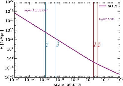
Figure 1. Expansion history of the $\mathrm{\Lambda }$CDM model computed using the Planck 2020 cosmological parameters. The vertical lines in blue bracket the epoch of big bang nucleosynthesis between neutron–proton freeze-out at $a_{\text{n/p}}\sim 1.3\cdot 10^{-10}$ and nuclei production at $a_{\text{nuc}}\sim 3.3\cdot 10^{-9}$, and the vertical lines in red indicate the time of matter–radiation equality $a_{\text{eq}}$, followed by recombination $a_{\text{rec}}$.

We observe a deceleration in the expansion rate $H$ in the course of the expansion of the universe, caused by gravity of the (attractive) components (see e.g., Peacock, 1999). It is important to note that no curvature term appears in $\mathrm{\Lambda }$CDM and space is considered flat. Hence, there should be no deceleration. On the other hand, there are gravitating energy densities in the universe, which should cause a curvature of space. This suggests that there is some “inconsistency” in $\mathrm{\Lambda }$CDM’s flat universe interpretation. We present an approach to resolve this inconsistency and discuss the consequences in the following sections. In a follow-up paper, we apply the concepts presented here onto nonlinear structure formation and investigate the impact of the formation of the cosmic web.

This paper is organized as follows. In Section 2, we recapitulate the basic equations for the evolution of the background universe in FLRW models. Section 3 investigates the flat universe interpretation for the general case of FLRW universes, followed by a discussion of the initial conditions (ICs) of the background universe. Section 4 proposes a $\mathrm{\Lambda }$CDM extension such that the cosmological model incorporates the post-big bang initial conditions of the early universe. Finally, in Section 5, we summarize the presented concepts, results, and implications, also in light of cosmological observations.

2 Basic equations for the expansion history in FLRW models

First, we recapitulate the well-known equations describing the evolution of the homogeneous and isotropic background universe that we need in our model. As gravity is the only force acting on cosmological length scales, it determines the evolution of the background universe and is described using Einsteins’ field equations:

$R_{\mu \nu }-\frac{1}{2}{g}_{\mu \nu }\mathcal{R}=\frac{8\pi G}{c^4}{T}_{\mu \nu },(1)$

with the Ricci tensor $R_{\mu \nu }$ and the Ricci scalar $\mathcal{R}$. The left-hand side (lhs) of the equation is often summarized as $E_{\mu \nu }$, the Einstein tensor. The right-hand side (rhs) contains the energy–momentum tensor $T_{\mu \nu }$, which includes the cosmic inventory of given cosmological models. The energy–momentum tensor $T_{\mu \nu }$ determines the curvature of space, expressed by the metric $g_{\mu \nu }$, which is also included in the Ricci tensor $R_{\mu \nu }$ and the Ricci scalar $\mathcal{R}$. Cosmological models differ in their assumptions on the nature and amount of the cosmic components encoded in $T_{\mu \nu }$. As such, all models are subject to observational constraints.

The geometry of a universe with constant curvature is described by applying the Riemannian formalism of curved surfaces and was developed by Robertson (1935), Robertson (1936a), Robertson (1936b), and Walker (1937) based on Milne’s idea of a kinematically determined universe (Milne, 1932) and preceding works by Friedmann (1922), Friedmann (1924), and Lemaître (1927). In spherical coordinates $(r,\theta ,\varphi )$, the line element of the metric reads as

$d{s}^2=c^{2}d{t}^2-R^2(t)\left(\frac{d{r}^2}{1-k{r}^2}+r^{2}d{\mathrm{\Omega }}^2\right),(\mathrm{2a})$

$d{\mathrm{\Omega }}^2=d{\theta }^2+{\sin }^2\theta d{\varphi }^2,(\mathrm{2b})$

with the curvature index $k$ and its values $+1$ (closed universe), 0 (flat universe), and $-1$ (open universe). The spatial coordinates $(r,\theta ,\varphi )$ are defined in the co-moving frame, where $r$, $\theta$, and $\varphi$ remain “fixed,” corresponding to the assumption of spaces of constant global curvature (the geometry of the universe). $R(t)$ is the “radius of curvature,” as described by Kolb and Turner (1990), at cosmic time $t$ (for $k=\pm 1$), with the dimension of length. Robertson calls this space an “auxiliary space,” and Walker calls it a “Riemannian space,” in contrast to Friedmann, who identifies it as the physical space of the universe.

Applying the FLRW metric Equation 2 to the metric tensor $g_{\mu \nu }$ in Einstein Equation 1, the energy–momentum tensor $T_{\mu \nu }$ then takes a perfect-fluid form, which reads

$T^{\mu \nu }=\left(\rho +\frac{p}{c^2}\right)u^{\mu }{u}^{\nu }-g^{\mu \nu }p,(3)$

where $u^{\mu }$ and $u^{\nu }$ is the four-velocity. The time–time component of the solution to Einstein Equation 1 yields the (first) Friedmann equation in the classical version, as derived by Friedmann (1922), see Section 3 and, for example, Kolb and Turner (1990):

$H^2\left(t\right)=\frac{8\pi G}{3c^2}\rho -\frac{k{c}^2}{a^2\left(t\right)},(4)$

which describes the dynamics of the evolution of the background universe in the reference frame of a free-falling observer, co-moving with the expansion³, moving on a geodesic (in a possibly curved space). Here, $\rho$ refers to the entire energy density of the universe; $k$ is the curvature index, defined in Equation 2 determining the geometry, with $k=+1$ for a closed (supercritical, density greater than the critical density) universe, $k=-1$ for an open (subcritical, density less than the critical density) universe, and $k=0$ for a flat geometry with critical density. In the following sections, we use the notion “geometry” for the curvature of the universe as determined by the FLRW metric (Equation 2) and the Friedmann Equation 4, respectively. $a$ denotes the scale factor, with the dimension of length, which owing to the symmetries imposed by the isotropy and homogeneity of the background universe is only a function of cosmic time $t$ and is defined as the “size” of an expanding or contracting universe, relative to its present-day size $|a_0|=1$. $H$ is the Hubble parameter (we use the term expansion rate interchangeably) defined as

$H\left(t\right)\equiv \frac{\dot{a}}{a},(5)$

where the dot refers to the derivative with respect to cosmic time $t$. The space–space component yields the second Friedmann equation as

$\frac{\ddot{a}}{a}=-\frac{4\pi G}{3c^2}\left(\rho +3p\right),(6)$

which Friedmann called the deceleration equation. In the recent literature, it is referred to as the acceleration equation.

Now, let us introduce the cosmic inventory that features the current concordance $\mathrm{\Lambda }$CDM model. In addition, we introduce some standard notions and equations that we need in the paper. The energy densities of interest include “CDM,” baryons (“b”), and radiation (“r”) (including photons and neutrinos). In the formulae, we also include the cosmological constant $\mathrm{\Lambda }$, empirically added to the cosmic inventory to explain the flatness of space, confirmed by the observations of the CMB, using the balloon-based BOOMERanG experiment (de Bernardis et al., 2000; MacTavish et al., 2006) as well as observations with increasing accuracy by the space missions COBE (Smoot et al., 1992), WMAP (Hinshaw et al., 2013), and Planck (Planck-Collaboration, 2020).

To study a variety of cosmological models, it has become customary to put “curvature” and the cosmological constant “$\mathrm{\Lambda }$” into the energy–momentum tensor $T_{\mu \nu }$ by operationally defining “effective” energy densities for them, namely, ${\rho }_k=-3k{c}^2/(8\pi G{a}^2)$ for curvature (“k”) and ${\rho }_{\mathrm{\Lambda }}=\mathrm{\Lambda }{c}^2/(8\pi G)$ for the cosmological constant.

We stress that although ${\rho }_k$ represents a geometric quantity, it has morphed into a “substance” or cosmic inventory, described by $T_{\mu \nu }$, upon this standard operational procedure⁴. Nevertheless, it is rightfully not regarded as a physical constituent of the universe (see Section 3.1) but simply a mathematical formalism, contributing an effective or artificial contribution to $T_{\mu \nu }$. On the other hand, in $\mathrm{\Lambda }$CDM, $\mathrm{\Lambda }$ is usually regarded as a real physical cosmic inventory, which contributes to $T_{\mu \nu }$, basically in the same manner as matter and radiation.

The Friedmann equation in modern language reads as

$\begin{array}{c}\hfill H^2\left(t\right)=\frac{8\pi G}{3c^2}\left[{\rho }_r\left(t\right)+{\rho }_b\left(t\right)+{\rho }_{\text{CDM}}\left(t\right)+\right.\\ \hfill \left.{\rho }_k\left(t\right)+{\rho }_{\mathrm{\Lambda }}\left(t\right)\right],\end{array}(7)$

with the time-dependent background energy densities for radiation $({\rho }_r)$, baryons $({\rho }_b)$, CDM $({\rho }_{\text{CDM}})$, the curvature $({\rho }_k)$, and the cosmological constant $({\rho }_{\mathrm{\Lambda }})$. $H(t)$ is the Hubble parameter, and its present-day value⁵, the Hubble constant, is denoted as $H_0$. The critical density, defining a flat universe (i.e., a universe with flat geometry), is given by

${\rho }_{\text{crit},t}=\frac{3H^2\left(t\right)c^2}{8\pi G},(8)$

which is derived from Equation 4 with a vanishing curvature term. It is convenient to introduce the so-called density parameters or cosmological parameters as

${\mathrm{\Omega }}_{i,t}=\frac{{\rho }_i\left(t\right)}{{\rho }_{\text{crit},t}},(9)$

where $i=$ CDM, b, r, etc., which are nothing but the background energy densities relative to the critical density (Equation 8).

To customarily solve the Friedmann equation, the energy conservation equation is applied (for each component, $i=$CDM, b, r, …), which reads

$\frac{\partial {\rho }_i}{\partial t}+3H\left({\rho }_i+p_i\right)=0,(10)$

where ${\rho }_i$ and $p_i$ stand for the background energy densities and pressures⁶, respectively. The energy densities and pressures are each related by their respective equation of state (EoS):

$p_i\left(t\right)=w_i\left(t\right){\rho }_i\left(t\right),(11)$

where $w_i$ is often called the EoS parameter, which can also change with time, in general. However, in $\mathrm{\Lambda }$CDM, $w_i$ is assumed to be a constant⁷ for every component $i=$CDM, b, r, $\mathrm{\Lambda }$, and k. Assuming a constant EoS parameter $w_i$ and substituting Equation 11 in Equation 10, it follows that $\dot{{\rho }_i}/{\rho }_i=-3(1+w_i)\dot{a}/a$, which is readily integrated to yield the well-known relationship:

${\rho }_i\left(a\right)={\mathrm{\Omega }}_{i,0}{\rho }_{\text{crit},0}{a}^{-3\left(1+w_i\right)},(12)$

which describes the evolution of the background energy densities as a function of the scale factor $a$ for the constant $w_i$. The background evolution of the standard cosmic components is thus given as

${\rho }_r(a)={\mathrm{\Omega }}_{r,0}{\rho }_{\text{crit},0}/a^4,(\mathrm{13a})$

${\rho }_m(a)={\mathrm{\Omega }}_{m,0}{\rho }_{\text{crit},0}/a^3,(\mathrm{13b})$

${\rho }_k(a)={\mathrm{\Omega }}_{k,0}{\rho }_{\text{crit},0}/a^2,(\mathrm{13c})$

${\rho }_{\mathrm{\Lambda }}={\mathrm{\Omega }}_{\mathrm{\Lambda },0}{\rho }_{\text{crit},0},(\mathrm{13d})$

where Equation 13a refers to the radiation component (its EoS parameter in Equation 11 is $w_r=1/3$), Equation 13b refers to baryonic matter and CDM $(w_m=0)$, Equation 13c refers to the curvature $(w_k=-1/3)$, and Equation 13d refers to the cosmological constant $\mathrm{\Lambda }$ $(w_{\mathrm{\Lambda }}=-1)$.

The Friedmann equation for the $\mathrm{\Lambda }$CDM model (Equation 7) can be alternatively written as an algebraic closure condition. In the present study, it reads

$1={\mathrm{\Omega }}_{r,0}+{\mathrm{\Omega }}_{b,0}+{\mathrm{\Omega }}_{\text{CDM},0}+{\mathrm{\Omega }}_{k,0}+{\mathrm{\Omega }}_{\mathrm{\Lambda },0}.(14)$

In other words, Equation 14 is the normalization of Friedmann Equation 7 to the critical density. In the $\mathrm{\Lambda }$CDM model, ${\mathrm{\Omega }}_{k,0}=0$ is prescribed such that $\mathrm{\Lambda }$ closes the universe to critical density, defining it a flat universe, which we elaborate in the next section.

3 The flat universe interpretation

The $\mathrm{\Lambda }$CDM model is a member of the broader family of FLRW cosmological models. Furthermore, a flat space in the universe is assumed on the grounds of the curvature of space, as measured, for example, by the observations of the CMB—the flat universe interpretation, where the curvature term in Friedmann Equation 4 is customarily interpreted to express the geometry of the universe. We will now reassess this interpretation.

3.1 Curvature in FLRW universes

Let us elaborate on the curvature term appearing in Friedmann Equation 4, which is connected to the curvature in the FLRW metric (Equations 2a,b). To this end, we now summarize the derivation of Friedmann Equation 4, see, for example, Kolb and Turner (1990). As mentioned above, Equation 4 is derived by applying the FLRW metric (Equations 2a,b) to the metric tensor $g_{\mu \nu }$ in Einstein Equation 1. The energy–momentum tensor (Equation 3) reads

$T_{\mu \nu }=diag\left(\rho ,-p,-p,-p\right),(15)$

The non-zero components of the Ricci tensor $R_{\mu \nu }$ for the FLRW metric (Equation 2) are determined as follows:

the time–time component as

$R_{00}=-3\frac{\ddot{a}}{a},(16)$

the space–space component as

$R_{ij}=-\left[\frac{\ddot{a}}{a}+2\frac{{\dot{a}}^2}{a^2}+\frac{2k}{a^2}\right]g_{ij},(17)$

and the Ricci scalar $\mathcal{R}$ as

$\mathcal{R}=-6\left[\frac{\ddot{a}}{a}+\frac{{\dot{a}}^2}{a^2}+\frac{k}{a^2}\right].(18)$

Using Equation 16 and Equation 18, the time–time component of the solution to Einstein Equation 1 yields

$\frac{{\dot{a}}^2}{a^2}+\frac{k}{a^2}=\frac{8\pi G}{3c^2}\rho ,(19)$

where $\rho$ is the energy density. In the above equation, the left-hand side stems from the Ricci scalar $\mathcal{R}$ (Equation 18), and the right-hand side $\rho$ comes from the time–time component of the energy–momentum tensor (Equation 15). Thus, the term $k/a^2$ does not contribute to $T_{\mu \nu }$ and has no impact on $g_{\mu \nu }$ in the solution to Equation 1 for a given choice of $T_{\mu \nu }$. Equation 19 is readily rewritten to (first) Friedmann Equation 4.

This suggests that the curvature term should not be confused with a contribution to the energy–momentum tensor, which determines the Riemann tensor in Einstein Equation 1. It is these equations which ought to determine the global curvature of space in the universe. We now reassess the interpretation of the curvature term in Equation 4 as the curvature of space in the universe using the Einstein–de Sitter (EdS) model (see also Section 1).

First, let us start from Einstein Equation 1 only, which describes the curvature of space, determined by the energy–momentum tensor $T_{\mu \nu }$ that describes the distribution of energy (or matter) in the universe. Applying $T_{\mu \nu }$ and solving Einstein Equation 1 yield the metric tensor $g_{\mu \nu }$, which describes the global curvature of space in the universe. Considering the EdS universe, we apply $T_{\mu \nu }=diag(\mathrm{1,0,0,0})$ with the density in units of critical density and zero pressure for pressureless matter, which yields a non-flat metric tensor $g_{\mu \nu }$. This is easily observed in a type of cross-check by solving the Friedmann equation for the EdS universe $H^2=(8\pi G/3c^2){\rho }_{\text{crit}}$, which yields $H^2(a)\propto a^{-3}$, given by Equation 13b. Thus, we observe a deceleration in the expansion rate $H$ during the expansion of the EdS universe, which is caused by gravity (see, e.g., Peacock, 1999). It is important to note that no curvature term appears in Equation 4 for the EdS universe. So there is curvature of space, although no curvature term exists in Equation 4 (i.e., there is curved space in a universe with flat geometry).

Now, the other direction follows the steps of the derivation of Friedmann Equation 4, as described above, and reverses the procedure of step 1. One starts by specifying the metric tensor $g_{\mu \nu }$ corresponding to the curvature term of Equation 4. Applying this metric tensor $g_{\mu \nu }$ to Einstein Equation 1 yields $T_{\mu \nu }$ with the corresponding energy densities⁸. The obtained energy–momentum tensors are checked for agreement with those we used in the previous step. Again, using the example of the EdS universe, we observe that the curvature term in Equation 4 vanishes for the EdS universe, and the corresponding metric tensor $g_{\mu \nu }$ describes flat space, which yields the energy–momentum tensor $T_{\mu \nu }=diag(\mathrm{0,0,0,0})$ of empty space. This is different from $T_{\mu \nu }=diag(\mathrm{1,0,0,0})$ for space at critical density in the EdS universe. Thus, in general, the curvature term does not express the spatial curvature⁹. This is addressed by Robertson (1936a), by using an “auxiliary” (mathematical) space associated with the FLRW metric (Equations 2a,b) (based on Riemannian geometry), which categorizes the dynamics of expansion of the background universe via the curvature index $k\in \left\{-1,+\mathrm{1,0}\right\}$ as open (negative curvature), closed (positive curvature), and flat (no curvature), based on the energy density of the background universe relative to the critical density¹⁰. Walker (1937) used the term “Riemannian space” for the space connected to the metric.

However, with regard to $\mathrm{\Lambda }$CDM, the question arises about how it is possible that observations of the CMB report the flatness of space, given that the universe is not empty. Friedmann Equation 4 describes the dynamics of the expansion of the background universe, expressed by the evolution of the expansion rate $H(t)$ in the local reference frame of observers co-moving with the expansion, moving on geodesics, that is, freely falling FLRW observers. The expansion rate $H(t)$ is determined by the two contributing terms describing the evolution of the density and the curvature, determined by Equation 13. A stringent consequence of GR’s equivalence principle is that observers, freely falling in a gravitational potential, reside in a local inertial system, during the entire evolution of the universe, where special relativity (SR) applies, that is, they perceive flat space [see, e.g., Weinberg (1972), Weinberg (2008), Peacock (1999), or Fließbach (2016)]. Moreover, a consequence of this is that space appears flat to co-moving FLRW observers, regardless of the energy density of the model universe. Thus, space appears flat to co-moving observers in open, closed, and flat geometries, justifying ${\rho }_k=0$ and ${\mathrm{\Omega }}_{k,0}=0$ in the $\mathrm{\Lambda }$CDM model, providing the reason for the observation of the flatness of space, not necessarily connected to the critical density. This again suggests that the curvature term in the Friedmann equations (Equation 4 and Equation 7) does not express the global spatial curvature, as determined by Einstein Equation 1 but the curvature of the auxiliary Riemannian space defined by Robertson (1936b) and Walker (1937). Nevertheless, the interpretation of the curvature term in Equation 4 is still a pending question as the term is not related to ${\rho }_k$ and ${\mathrm{\Omega }}_{k,0}$, which express the observed flatness of space by us as free-falling FLRW observers. We fulfill the criterion of being co-moving FLRW observers not strictly (Peacock, 1999) but to a very high degree (details in a follow-up paper).

Equations 4, 6, 10 describe the expansion history of the background universe. These equations are not independent of each other. It is well known that first Friedmann Equation 4 is the result of the integration of second Friedmann Equation 6. We multiply Equation 6 by the scale factor $a$ to derive

$\ddot{a}=-\frac{4\pi G}{3c^2}\left(\rho +3p\right)a,(20)$

which we integrate with respect to time, at which we consider the energy conservation Equation 10, yielding

${\dot{a}}^2=\frac{8\pi G{a}^2}{3c^2}\rho -k{c}^2,(21)$

where $k$ appears as an integration constant. Dividing by $a^2$ recovers first Friedmann Equation 4, being an ordinary differential equation. Therefore, the integration constant $k$ can be determined from the ICs, which we elaborate next.

3.2 The initial conditions of FLRW universes

Customarily, the geometry (open, closed, or flat) of a model universe is explained based on the energy density of the background universe relative to the critical density. We present a more general definition based on the ICs of the background universe, comprising the initial densities in the early universe and the initial (post-big bang) expansion rate.

The expansion rate for a universe at critical density is described by the Friedmann equation with the vanishing curvature term as

$H^2\left(t\right)=\frac{8\pi G}{3c^2}{\rho }_{\text{crit},t}.(22)$

This relationship between the expansion rate $H$ and ${\rho }_{\text{crit}}$ holds true for the entire cosmic time, especially in the very first moments after the big bang. More precisely, the initial boost in the expansion rate is supposed to be provided immediately after the big bang. By the time we can apply GR, we can define an initial expansion rate $H_{\text{ini}}$ (in the language of Lemaître, we could call it here “the primeval expansion rate”). At this cosmic point in time, when it becomes meaningful to apply the Friedmann equation, the universe experienced its first deceleration phase (see, e.g., Harrison, 2000), and the metric would appear flat to a co-moving FLRW observer.

On the other hand, we can express the critical density for a flat universe as

${\rho }_{\text{crit,ini}}=\frac{3H_{\text{ini}}^2{c}^2}{8\pi G},(23)$

which is simply the rearrangement of Equation 22 to express ${\rho }_{\text{crit}}$ at the considered initial point in time. This defines the “critical expansion rate,” for a given initial density as

$H_{\text{crit,ini}}^2=\frac{8\pi G}{3c^2}{\rho }_{\text{ini}}.(24)$

We can interpret this relationship as follows. Given an arbitrary initial energy density ${\rho }_{\text{ini}}$ of a universe, originating from the big bang, the primeval expansion rate $H_{\text{ini}}$ has to be specifically fine-tuned to fulfill the criterion (Equation 24) describing a universe with flat geometry, that is, $H_{\text{ini}}=H_{\text{crit,ini}}$.

However, there are no comprehensible arguments for why the big bang should be restricted to this exclusive fine-tuned value for $H_{\text{ini}}$. If $H_{\text{ini}}$ is less than $H_{\text{crit,ini}}$ (or in other words, ${\rho }_{\text{ini}}$ is higher than ${\rho }_{\text{crit,ini}}$, fulfilling Equation 24), the evolution of the universe is described by a closed geometry. An open geometry is determined by $H_{\text{ini}}$ greater than $H_{\text{crit,ini}}$ (or ${\rho }_{\text{ini}}$ being lower than ${\rho }_{\text{crit,ini}}$, fulfilling Equation 24).

Limiting ourselves to a flat geometry and given the energy densities as deduced by the measurements of the CMB [e.g., by Planck-Collaboration (2020)] in $\mathrm{\Lambda }$CDM, it thereby ignores from the outset a broad range of possible initial expansion rates $H_{\text{ini}}$. Hence, the assumption of a flat geometry in the FLRW metric does not cover those initial expansion rates $H_{\text{ini}}$, which would lead to subcritical and supercritical universes, where, as shown in Section 3.1, freely falling, co-moving observers likewise perceive flat space.

4 Incorporating the post-big bang initial conditions

In Section 3.1, we argue that a prospective observation of flat space does not necessarily imply a universe at critical density since the curvature terms ${\rho }_k$ and ${\mathrm{\Omega }}_k$ in Equations 7, 14, respectively, vanish in the local inertial frame of co-moving FLRW observers, giving the reasons for the flatness of space as measured by the observations of the CMB. To interpret the curvature term in Equation 4, we associate the general concept of dark energy (DE) with the geometry of the FLRW metric (Equations 2a,b) and use the subscript “de” for the quantities describing the dynamics of expansion in the following section.

In Section 3.2, we argue that the ICs of the background universe are given by the initial expansion rate $H_{\text{ini}}$ and the initial densities. Based on the CMB measurements, within the $\mathrm{\Lambda }$CDM model, the initial densities are determined to high precision (see also Foidl and Rindler-Daller, 2024). For this reason, it is sufficient to incorporate $H_{\text{ini}}$ into the $\mathrm{\Lambda }$CDM formalism. Let us proceed in our approach by considering the following parameters:

$1={\mathrm{\Omega }}_{r,0}+{\mathrm{\Omega }}_{b,0}+{\mathrm{\Omega }}_{\text{CDM},0}+{\mathrm{\Omega }}_{k,0}+{\mathrm{\Omega }}_{\text{de},0},(25)$

where the operationally defined density parameter of the geometrical curvature ${\mathrm{\Omega }}_{\text{de}}$ takes the place of ${\mathrm{\Omega }}_{\mathrm{\Lambda }}$. For the sake of completeness, we include ${\mathrm{\Omega }}_{k,0}(=0)$ in the equation to express the perceived flatness of space. In the same way as in $\mathrm{\Lambda }$CDM, ${\mathrm{\Omega }}_{k,0}=0$ describes the flatness of space but based on novel arguments as it appears to us in our local reference frame as co-moving FLRW observers.

To proceed with our approach, in an inflationary big bang cosmology, we allow for the following simplification. We analyze the evolution of cosmological models by the time inflation has ended, and we call the expansion rate at the end of inflation “primordial expansion rate” (in analogy to the primordial power spectrum in structure formation). Detailed information of the exact evolution of $H$ prior to this point is not required.

We recognize from Equation 25 that

${\mathrm{\Omega }}_{\text{de},0}=1-{\mathrm{\Omega }}_{\text{phys},0},(26)$

where ${\mathrm{\Omega }}_{\text{phys},0}$ denotes the sum total of the density parameters (${\mathrm{\Omega }}_{\text{CDM},0}$, ${\mathrm{\Omega }}_{b,0}$, and ${\mathrm{\Omega }}_{r,0}$) of all physical contributions to the energy budget of the universe (CDM, baryons, and radiation; without considering the operationally defined contributions to the energy–momentum tensor $T_{\mu \nu }$).

We want to use the EoS parameter $w_{\text{de}}$ of ${\rho }_{\text{de}}$ to parameterize the dynamics of the expansion, determined by the curvature term in Equation 4, as a function of the sum total of the energy densities of the cosmic components in the universe ${\mathrm{\Omega }}_{\text{phys}}$, that is, relate it to Equation 25. This retains the customary $\mathrm{\Lambda }$CDM formalism, although we are only left to adapt the computation of $w_{\text{de}}$, instead of using the constant EoS parameter $w_{\mathrm{\Lambda }}=-1$ of the $\mathrm{\Lambda }$CDM model.

To this end, we carried out a change in variable $\rho$ in Equation 4 to ${\mathrm{\Omega }}_{\text{phys}}$: we multiply Equation 4 by $a^2(t)$, divide it by 2, and use the total amount of energy $(4\pi /3){\rho }_{\text{phys}}{a}^3$ in the sphere of “radius” (scale factor) $a$, in units of the critical density (see Equation 26), instead of the respective energy density ${\rho }_{\text{phys}}$, which yields

$\frac{1}{2}{\dot{a}}^2\left(t\right)-\frac{G{\mathrm{\Omega }}_{\text{phys}}}{a}=\kappa ,(27)$

with the constant $\kappa$.

We now use Equation 27 to determine $w_{\text{de}}$ as follows. Since $\kappa$ is a constant, the evolution of the first term is determined by the evolution of the second term, given by

$\frac{d}{da}\left(\frac{G{\mathrm{\Omega }}_{\text{phys}}}{a}\right)\propto -\frac{{\mathrm{\Omega }}_{\text{phys}}}{a^2},(28)$

where we use the fact that all the cosmic components of interest evolve smoothly with respect to the scale factor $a$, as observed by the power laws in Equation 13, just as in $\mathrm{\Lambda }$CDM. Moreover, this is unsurprisingly equivalent to Equation 13c, which is derived from Equation 12. In what follows, we do not need detailed prefactors. We use the right-hand side of Equation 28 in Equation 12, which yields

${\rho }_{\text{de}}\propto a^{-2{\mathrm{\Omega }}_{\text{phys},0}}.(29)$

To transform the variables back to the customarily used energy density ${\rho }_{\text{de}}$, we equate the exponents in Equation 12, 29 by $-3(1+w_{\text{de}})=-2{\mathrm{\Omega }}_{\text{phys},0}$. Rearranged to express $w_{\text{de}}$, it reads as

$w_{\text{de}}=\frac{2}{3}{\mathrm{\Omega }}_{\text{phys},0}-1,(30)$

where $w_{\text{de}}$ is a constant.

The significant property of Equation 30 is that in general, it does not yield the EoS of a cosmological constant. Only for an empty universe, we get exactly $w_{\text{de}}=-1$. In fact, this is in good accordance with the original empty de Sitter universe solution (de Sitter, 1917) and the expectations from a kinematically determined universe: if the universe is empty, there is no global curvature of space and hence no deceleration but rather $H=const$, resulting in an exponential growth of the scale factor.

However, as soon as we have physical components, ${\mathrm{\Omega }}_{\text{phys},0}>0$, the EoS parameter in Equation 30 fulfills $w_{\text{de}}>-1$. If we choose the same matter content as the $\mathrm{\Lambda }$CDM concordance model, that is, using ${\mathrm{\Omega }}_{\text{phys},0}\approx {\mathrm{\Omega }}_{m,0}\simeq 0.3$, Equation 30 yields $w_{\text{de}}\simeq -0.8$; thus, there is a weak deceleration compared to a model with $w_{\mathrm{\Lambda }}=-1$. Still, the two EoS parameters are close numerically and in terms of their phenomenological impact onto the expansion history (which we present in detail in a follow-up paper).

On the other hand, a universe at critical density, that is, ${\mathrm{\Omega }}_{\text{phys},0}=1$, yields $w_{\text{de}}=-1/3$, which is the EoS parameter of the spatial curvature used in the FLRW formalism and restricted to the fine-tuned case of a universe at critical density. This is exactly what we expect.

To retain $\mathrm{\Lambda }$CDM’s formalism and Equation 12, we make a distinction of cases. We apply the constant value of $w_{\text{de}}=-1/3$ to flat and closed geometries, as is also the case in $\mathrm{\Lambda }$CDM (with $w_k=-1/3$). For open geometries, we apply Equation 30. In summary, we have

$w_{\text{de}}=-\frac{1}{3}-\mathrm{\Theta }({\mathrm{\Omega }}_{\text{de},0})\frac{2}{3}{\mathrm{\Omega }}_{\text{de},0},(\mathrm{31a})$

$\begin{array}{l}\hfill \\ \hfill {\mathrm{\Omega }}_{\text{de},0}& =1-{\mathrm{\Omega }}_{\text{phys},0},\hfill \end{array}(\mathrm{31b})$

where in Equation 31a $\mathrm{\Theta }$ is the Heaviside function. The EoS parameter $w_{\text{de}}$ is a function of ${\mathrm{\Omega }}_{\text{de},0}$ (see Equation 31b) and therefore a constant for a given sum total of physical energy densities. The Heaviside function separates the two regimes of super- and subcritical model universes. The first term corresponds to deceleration due to the critical density. The factor after the Heaviside function applies to subcritical universes only, where $w_{\text{de}}$ falls below $-1/3$; that is, a decreasing EoS parameter implies less deceleration as it should. In addition, we retain ${\mathrm{\Omega }}_{k,0}=0$ to express the perceived flatness of space in our local inertial frame as co-moving FLRW observers, just the same way as in $\mathrm{\Lambda }$CDM. This is essential to the linear perturbation theory applied in $\mathrm{\Lambda }$CDM, for example, in the calculation of the CMB temperature spectrum, as the notion “curvature” herein refers to spatial curvature in the Einstein equations (see, e.g., Ma and Bertschinger, 1995; Weinberg, 2008; Coles and Lucchin, 2002; Mukhanov 2005; Dodelson, 2003; Peebles, 1993), and not to the geometry of the FLRW metric. A description of how the spatial curvature affects the CMB temperature spectrum can be found in many textbooks covering structure formation (see the aforementioned references). However, there is a degeneracy for the impact of spatial curvature on the CMB spectrum with the cosmological constant $\mathrm{\Lambda }$ or dark energy, respectively (see, e.g., Hu and Dodelson, 2002). We will explain this point in a follow-up paper.

Finally, the Friedmann Equation 32a reads

$H^2(t)=\frac{8\pi G}{3c^2}\left[{\rho }_r(t)+{\rho }_b(t)+{\rho }_{\text{CDM}}(t)\right.\left.+{\rho }_{\text{de}}(t)\right],(\mathrm{32a})$

${\rho }_{\text{de}}(a)={\mathrm{\Omega }}_{\text{de},0}{\rho }_{\text{crit},0}{a}^{-3(1+w_{\text{de}})},(\mathrm{32b})$

where Equation 32b now describes the evolution of ${\rho }_{\text{de}}$ as a function of scale factor $a$ for a constant $w_{\text{de}}$, given by Equation 31. The present-day critical density ${\rho }_{\text{crit},0}$ is defined in Equation 8.

Figure 2 finally displays the time evolution of the scale factors of model universes with various matter densities, color-coded by density parameter ${\mathrm{\Omega }}_m$, whose value refers to the present, within our $\mathrm{\Lambda }$CDM extension. The red curves indicate universes with closed geometry; the yellow curve has exactly the critical density, that is, the EdS universe, which separates the supercritical from the subcritical universes, which go from light green to deep blue for the empty universe.

Figure 2

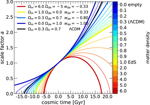
Figure 2. Expansion histories of model universes with the kinematical DE component. The color-coded curves display the expansion history of individual model universes applying Equations 4, 31 for models with supercritical density (dark red), the EdS model (yellow), and the empty de Sitter universe (dark blue). The black curve indicates the expansion history of the $\mathrm{\Lambda }$CDM model with ${\mathrm{\Omega }}_m=0.3$ and ${\mathrm{\Omega }}_{\mathrm{\Lambda }}=0.7$, assuming a cosmological constant, i.e., $w_{\mathrm{\Lambda }}=-1$. We see a great similarity comparing $\mathrm{\Lambda }$CDM to the model shown for the same matter density and ${\mathrm{\Omega }}_{\text{de}}=0.7$ (thick light blue curve). This model displays the same characteristic s-shape, indicating the transition from decelerated to accelerated expansion because of $w_{\text{de}}=-0.8$ being “close” to a cosmological constant, given the relatively low energy density observed in the universe.

The curves between the yellow and the dark blue curves depict the evolution of subcritical models with matter densities between the EdS model with critical density (solid yellow curve) and the empty model (solid dark blue curve). We can observe that the cosmological models transition uniformly between these two limiting model cases, corresponding to decreasing mass density and “approaching” the exponential curve of the empty model, exactly as expected for kinematically determined universes in GR. In fact, a universe filled with a cosmological constant to critical density displays the same evolution as the expectations for an empty universe, in the former by negative pressure balancing gravity¹¹ and in the latter by vanishing gravity in an empty universe.

The black solid curve indicates the evolution of the $\mathrm{\Lambda }$CDM model with ${\mathrm{\Omega }}_m=0.3$ and the cosmological constant ${\mathrm{\Omega }}_{\mathrm{\Lambda }}=0.7$. Comparing it to the solution obtained by our $\mathrm{\Lambda }$CDM extension with ${\mathrm{\Omega }}_{\text{de}}=0.7$ and $w_{\text{de}}=-0.8$ for a model universe with an identical amount of matter ${\mathrm{\Omega }}_m=0.3$ (thick solid light blue curve), we recognize the similarity between both models. Both display the typical s-shape in the evolution of the scale factor, indicating the transition from decelerated to accelerated expansion, known from $\mathrm{\Lambda }$CDM. However, there is a difference in the age between the two world models. We discuss this finding and other features, along with the results of further calculations in detail in a follow-up paper. Moreover, the evolution of supercritical model universes with matter densities above the critical density also matches the expectation. They display no deviations from conventional computations, with respect to the evolution of their scale factors.

Our approach shows a significant difference compared to the cosmological constant $\mathrm{\Lambda }$, which is considered a physical content of the universe. However, unlike the cosmological constant $\mathrm{\Lambda }$, ${\rho }_{\text{de}}$ here does not contribute to the energy budget of the universe; instead, it refers to a kinematic effect, described by an effective DE component emerging from the geometry of the FLRW metric. As such, it is considered an operational contribution to the energy–momentum tensor and is not regarded as a physical contribution to the universe, as depicted in Equation 19, just in the same way as ${\rho }_k$ in $\mathrm{\Lambda }$CDM obviously. Although it seems to be only a minor modification, it brings a significant difference compared to the $\mathrm{\Lambda }$CDM model as the universe, in this approach, is considered an open universe with subcritical energy density and the sum total of the energy densities of the physical contributions (radiation and matter) to the energy budget of the universe is below critical density. Finally, ${\mathrm{\Omega }}_{k,0}=0$ refers to the perceived flatness of space in the local inertial system of the co-moving FLRW observer, in contrast to $\mathrm{\Lambda }$CDM, where it is interpreted as the global flatness of space.

5 Summary and conclusion

We first presented the historical context of the foundation of modern cosmology: the Einstein equations and the FLRW metric. The geometric interpretation of gravity describes it as the dynamical curvature of space by gravitating masses (more precisely, gravitating energy densities¹²). Based on Milne’s idea of a kinematically determined universe, Robertson and Walker derived the FLRW metric. Applying this metric to the Einstein equations yields the Friedmann equation, which describes the evolution of the expansion history of a kinematically determined universe in the reference frame of observers co-moving with the expansion: they move on geodesics; i.e., they are free-falling. The expansion of the universe started with a very high expansion rate, which is continuously decelerated due to the action of gravity: the kinematic determination of the evolution of the universe. We presented three examples of model universes, which suggested that there might be some “incompleteness” in $\mathrm{\Lambda }$CDM’s flat universe interpretation. Our proposal to solve this incompleteness includes the following novelties:

a. We take the concept of a kinematically determined universe, the equivalence principle, and the concept of the co-moving FLRW observer at face value and find that the FLRW metric and the curvature of space are two individual aspects of the geometry of the universe, where we identify the geometry given by the FLRW metric with a kinematic DE component.

b. In the FLRW formalism, the density parameters of subcritical and supercritical universes are also normalized to critical density by considering the suitable amount of spatial curvature. In contrast to this, we consider the consequence of the equivalence principle that irrespective of the geometry (open, closed, or flat) of a universe, co-moving FLRW observers in their reference frame always perceive flat space. Thus, co-moving (i.e., free-falling) observers in subcritical universes, supercritical universes, or universes at critical density likewise perceive spatial flatness.

c. The FLRW formalism and therefore also $\mathrm{\Lambda }$CDM consider the energy densities in the early universe as the initial conditions determining the expansion history of the universe. In contrast, we consider these initial energy densities in relation to the post-big bang expansion rate as the initial conditions as a consequence of the kinematic determination of the universe. The relationship between these two quantities determines the geometry of the universe, as described by the curvature of the FLRW metric.

Owing to the different evolution of ${\rho }_{\text{de}}$ in our approach versus $\mathrm{\Lambda }$ in $\mathrm{\Lambda }$CDM, there is a difference in the age of the models, namely, 13.04 Gyr versus 13.8 Gyr, respectively. We checked to see that the younger age of our model is not in conflict with age estimates of the oldest known stars. It is also not in conflict with the very early galaxies found through the James Webb Space Telescope since the redshift determinations of these galaxies require a cosmological model to convert redshift into age. In our model, these galaxies would be correspondingly younger than those in a $\mathrm{\Lambda }$CDM universe. In a follow-up paper, we present an in-depth comparison with observations.

We first motivated our approach presented in this article by placing the key concepts of modern cosmology in a historical context. We now want to complete this view of the historical context. Although Robertson and Walker showed that observers co-moving with the expansion of the universe move on geodesics, they neither emphasized that they are in a locally flat space nor discussed the consequences. Unlike Friedmann, however, they describe the curvature of an auxiliary Riemannian space, not the physical space of the universe. In the closing statement of his works (Friedmann, 1922; Friedmann, 1924), Friedmann concluded that it is not possible to determine, based on the Einstein equations alone, whether the universe is finite (i.e., has supercritical density) or infinite (i.e., has critical or subcritical density) and that supplementary assumptions are required. Lemaître concluded that the universe originated from an event nowadays known as the big bang and has been expanding ever since; this is precisely this supplementary assumption Friedmann referred to. Considering the concept of a kinematically determined universe, we presented the idea that not only the initial density but also its relationship with the initial expansion rate determines the expansion history of the universe. This led to a very natural explanation for the phenomenology of a late-time accelerated expansion as a kinematic effect, which we incorporated into the FLRW formalism as a kinematical DE component.

Data availability statement

The original contributions presented in the study are included in the article/supplementary material, further inquiries can be directed to the corresponding authors.

Author contributions

HF: Conceptualization, Investigation, Methodology, Software, Visualization, Writing – original draft, Writing – review and editing. TR-D: Formal Analysis, Funding acquisition, Supervision, Writing – original draft, Writing – review and editing.

Funding

The author(s) declare that financial support was received for the research and/or publication of this article. TR-D acknowledges the support by the Austrian Science Fund FWF through the FWF Single-Investigator Grant (FWF-Einzelprojekt; grant no. P36331-N) and the hospitality of the Wolfgang Pauli Institute.

Acknowledgments

The authors are grateful to Glenn van de Ven, Paul Shapiro, Dragan Huterer, Oliver Hahn, and Bodo Ziegler for helpful and valuable discussions, concerning an earlier version of this manuscript.

Conflict of interest

The authors declare that the research was conducted in the absence of any commercial or financial relationships that could be construed as a potential conflict of interest.

Generative AI statement

The author(s) declare that no Generative AI was used in the creation of this manuscript.

Any alternative text (alt text) provided alongside figures in this article has been generated by Frontiers with the support of artificial intelligence and reasonable efforts have been made to ensure accuracy, including review by the authors wherever possible. If you identify any issues, please contact us.

Publisher’s note

All claims expressed in this article are solely those of the authors and do not necessarily represent those of their affiliated organizations, or those of the publisher, the editors and the reviewers. Any product that may be evaluated in this article, or claim that may be made by its manufacturer, is not guaranteed or endorsed by the publisher.

Footnotes

¹In fact, this normalization is just a convention.

²The curvature term is not regarded as a physical constituent of the universe; see Section 2. Hence, the model universe is empty.

³The co-moving observer is called fundamental observer by Robertson (1935). This term is also sometimes used in the literature.

⁴This goes back to a proposal by Zeldovich to simplify cosmological equations; see Zeldovich and Novikov (1983).

⁵The literature has adopted the notational subscript “0” to denote present-day values and not the values at $t=0$.

⁶This equation assumes that there is no transformation between different components.

⁷However, for a detailed study of phase transitions in the early universe, it is important to include a variable EoS of the radiation component to take into account the reduction in relativistic degrees of freedom in the wake of the universe’s expansion.

⁸In general, this solution is not unique.

⁹To falsify the assumption that the curvature term in Equation 4 expresses the curvature of space, one contradicting example is sufficient.

¹⁰As already mentioned in Section 1, the definition of $k$ refers to the density, although the density does not appear in the metric. In the FLRW formalism, this is addressed by normalized Friedmann Equation 14, relating density and curvature. Consequently, in the FLRW formalism, the density parameters of subcritical and supercritical universes are also normalized to critical density, for example, by considering the suitable amount of curvature. Remember that the curvature is not regarded as a physical contribution to the energy budget of the universe.

¹¹Of course, this scenario also applies to the inflationary phase of the universe, with $p\approx -\rho$ of the inflaton field dominating the universe, resulting in an exponential growth of the scale factor.

¹²The cosmological constant, for example, is not a gravitating type of energy as its negative pressure counteracts the effect of gravity.

References

Chodorowski, M. J. (2005). Cosmology under Milne’s shadow. Publ. Astron. Soc. Aust. 22, 287–291. doi:10.1071/AS05016

CrossRef Full Text | Google Scholar

Coles, P., and Lucchin, F. (2002). Cosmology: the origin and evolution of cosmic structure, second edition. Wiley-VCH, July.

Google Scholar

Davis, T. M., and Lineweaver, C. H. (2004). Expanding confusion: common misconceptions of cosmological Horizons and the superluminal expansion of the universe. Publ. Astron. Soc. Aust. 21, 97–109. doi:10.1071/AS03040

CrossRef Full Text | Google Scholar

de Bernardis, P., Ade, P. A. R., Bock, J. J., Bond, J. R., Borrill, J., Boscaleri, A., et al. (2000). A flat universe from high-resolution maps of the cosmic microwave background radiation. Nature 404, 955–959. doi:10.1038/35010035

PubMed Abstract | CrossRef Full Text | Google Scholar

de Sitter, W. (1916). On Einstein's theory of gravitation and its astronomical consequences. First paper. MNRAS 76, 699–728. doi:10.1093/mnras/76.9.699

CrossRef Full Text | Google Scholar

de Sitter, W. (1917). On the relativity of inertia. Remarks concerning Einstein’s latest hypothesis. K. Ned. Akad. Wet. Proceedings Series B Phys. Sci. 19, 1217–1225.

Google Scholar

Dodelson, S. (2003). Modern cosmology. Academic Press.

Google Scholar

Einstein, A. (1905). Zur Elektrodynamik bewegter Körper. Ann. Phys. 322, 891–921. doi:10.1002/andp.19053221004

CrossRef Full Text | Google Scholar

Einstein, A. (1915). “Die Feldgleichungen der Gravitation,” in Sitzungsberichte der Königlich Preußischen Akademie der Wissenschaften, 844–847.

Google Scholar

Einstein, A. (1917). “Kosmologische Betrachtungen zur allgemeinen Relativitätstheorie,”. Sitzungsberichte Königlich Preußischen Akad. Wiss. 142–152.

Google Scholar

Fließbach, T. (2016). Allgemeine relativitätstheorie. Springer Spektrum. doi:10.1007/978-3-662-53106-8

CrossRef Full Text | Google Scholar

Foidl, H., and Rindler-Daller, T. (2024). A proposal to improve the accuracy of cosmological observables and address the Hubble tension problem. A&A 686, A210. doi:10.1051/0004-6361/202348955

CrossRef Full Text | Google Scholar

Friedmann, A. (1922). Über die Krümmung des Raumes. Z. fur Phys. 10, 377–386. doi:10.1007/BF01332580

CrossRef Full Text | Google Scholar

Friedmann, A. (1924). Über die Möglichkeit einer Welt mit konstanter negativer Krümmung des Raumes. Z. fur Phys. 21, 326–332. doi:10.1007/BF01328280

CrossRef Full Text | Google Scholar

Harrison, E. R. (2000). Cosmology. The science of the universe. Cambridge University Press.

Google Scholar

Hinshaw, G., Larson, D., Komatsu, E., Spergel, D. N., Bennett, C. L., Dunkley, J., et al. (2013). Nine-year Wilkinson microwave anisotropy probe (WMAP) observations: cosmological parameter results. ApJS 208, 19. doi:10.1088/0067-0049/208/2/19

CrossRef Full Text | Google Scholar

Hu, W., and Dodelson, S. (2002). Cosmic microwave background anisotropies. ARA&A 40, 171–216. doi:10.1146/annurev.astro.40.060401.093926

CrossRef Full Text | Google Scholar

Hubble, E. (1929). A relation between distance and radial velocity among extra-galactic nebulae. Proc. Natl. Acad. Sci. 15, 168–173. doi:10.1073/pnas.15.3.168

PubMed Abstract | CrossRef Full Text | Google Scholar

Kolb, E. W., and Turner, M. S. (1990). The early universe, 69. Boca Raton, FL: Taylor & Francis Group

Google Scholar

Lemaître, G. (1927). Un univers homogène de masse constante et de rayon croissant rendant compte de la vitesse radiale des nébuleuses extra-galactiques. Ann. la Société Sci. Brux. 47, 49–59.

Google Scholar

Ma, C.-P., and Bertschinger, E. (1995). Cosmological perturbation theory in the synchronous and conformal newtonian gauges. ApJ 455, 7. doi:10.1086/176550

CrossRef Full Text | Google Scholar

MacTavish, C. J., Ade, P. A. R., Bock, J. J., Bond, J. R., Borrill, J., Boscaleri, A., et al. (2006). Cosmological parameters from the 2003 flight of BOOMERANG. ApJ 647, 799–812. doi:10.1086/505558

CrossRef Full Text | Google Scholar

Milne, E. A. (1932). World structure and the expansion of the universe. Nat. 130 (3270), 9–10. doi:10.1038/130009a0

CrossRef Full Text | Google Scholar

Mukhanov, V. (2005). Physical foundations of cosmology. Cambridge University Press. doi:10.2277/0521563984

CrossRef Full Text | Google Scholar

Peacock, J. A. (1999). Cosmological physics. Cambridge University Press. doi:10.1017/CBO9780511804533

CrossRef Full Text | Google Scholar

Peebles, P. J. E. (1993). Principles of physical cosmology. Princeton University Press.

CrossRef Full Text | Google Scholar

Planck-Collaboration Akrami, Y., Arroja, F., Ashdown, M., Aumont, J., Baccigalupi, C., et al. (2020). Planck 2018 results. I. Overview and the cosmological legacy of Planck. A&A 641, A1. doi:10.1051/0004-6361/201833880

CrossRef Full Text | Google Scholar

Robertson, H. P. (1935). Kinematics and world-structure. ApJ 82, 284. doi:10.1086/143681

CrossRef Full Text | Google Scholar

Robertson, H. P. (1936a). Kinematics and world-structure ii. ApJ 83, 187. doi:10.1086/143716

CrossRef Full Text | Google Scholar

Robertson, H. P. (1936b). Kinematics and world-structure iii. ApJ 83, 257. doi:10.1086/143726

CrossRef Full Text | Google Scholar

Schwarzschild, K. (1916). “On the gravitational field of a mass point according to Einstein’s theory,” in Sitzungsberichte der Königlich Preussischen Akademie der Wissenschaften zu Berlin. 189–196.

Google Scholar

Smoot, G. F., Bennett, C. L., Kogut, A., Wright, E. L., Aymon, J., Boggess, N. W., et al. (1992). Structure in the COBE differential microwave radiometer first-year maps. ApJ 396, L1. doi:10.1086/186504

CrossRef Full Text | Google Scholar

Walker, A. G. (1937). On Milne’s theory of world-structure. Proc. Lond. Math. Soc. 42, 90–127. doi:10.1112/plms/s2-42.1.90

CrossRef Full Text | Google Scholar

Weinberg, S. (1972). Gravitation and cosmology: principles and applications of the general theory of relativity. John Wiley and Sons, Inc.

Google Scholar

Weinberg, S. (2008). Cosmology. Oxford, UK: Oxford University Press.

Google Scholar

Zeldovich, I. B., and Novikov, I. D. (1983). “Relativistic astrophysics,”, Vol. 2. Revised: University of Chicago Press.

Google Scholar