Modeling ring current proton distribution using MLP, CNN, LSTM, and transformer networks

Li, Jinxing; Bortnik, Jacob; Wang, Qiushuo; Wu, Yingnian; Lizarraga, Andrew; Angel, Mirana; Wang, Beibei; Wen, Qianzhuang; Jiang, Jeffrey

doi:10.3389/fspas.2025.1629056

ORIGINAL RESEARCH article

Front. Astron. Space Sci., 01 October 2025

Sec. Space Physics

Volume 12 - 2025 | https://doi.org/10.3389/fspas.2025.1629056

This article is part of the Research TopicPredicting Near-Earth Space Environment: New Perspective and Capabilities in the AI AgeView all 4 articles

Modeling ring current proton distribution using MLP, CNN, LSTM, and transformer networks

Jinxing Li¹*^†

Jacob Bortnik¹^†

Qiushuo Wang¹^†

Yingnian Wu²

Andrew Lizarraga²

Mirana Angel³

Beibei Wang⁴^†

Qianzhuang Wen⁵^†

Jeffrey Jiang⁶

¹Department of Atmospheric and Oceanic Sciences, University of California, Los Angeles, CA, United States
²Department of Statistics and Data Science, University of California, Los Angeles, CA, United States
³University of California, Irvine, CA, United States
⁴CreatiAI, Los Angeles, CA, United States
⁵University of California, Riverside, CA, United States
⁶The Hun School of Princeton, Princeton, NJ, United States

This study aims at developing ring current proton flux models using four neural network architectures: a multilayer perceptron (MLP), a convolutional neural network (CNN), a long short-term memory (LSTM) network, and a Transformer network. All models take time sequences of geomagnetic indices as inputs. Experimental results demonstrate that the LSTM and Transformer models consistently outperform the MLP and CNN models by achieving lower mean squared errors on the test set, possibly due to their intrinsic capability to process temporal sequential input data. Unlike MLP and CNN models, which require a fixed input history length even though proton lifetime varies with altitude, the LSTM and Transformer models accommodate variable-length sequences during both training and inference. Our findings indicate that the LSTM and Transformer architectures are well suited for modeling ring current proton behavior when GPU resources are available, and the Transformer slightly underperforms the LSTM model due to the restriction on the number of total heads. For resource-constrained environments, however, the MLP model offers a practical alternative, with faster training and inference times, while maintaining competitive accuracy.

1 Introduction

The Earth’s magnetosphere is a highly dynamic system, and ring current ions are one of the most significant components of the magnetospheric environment. Accurate modeling of ring current dynamics is therefore crucial for space weather forecasting. Early studies with Explorer-45 captured the intensification and decay of ring current ions, and identified that the ring current lifetime is subject to charge exchange (Smith et al., 1981). AMPTE/CCE measurements with composition distributions clarified the relative roles of H+ and O+ in the ring current (Hamilton et al., 1988). Energetic neutral atom (ENA) imagers from the IMAGE and TWINS missions showed the influence of interplanetary magnetic field and geomagnetic field variation on global ring current ion dynamics (Brandt et al., 2002; Fok et al., 2010). Van Allen Probes measured ring current ion distributions with species-, energy-, and pitch-angle-resolutions throughout storm phases (e.g., Yue et al., 2017a; Yue et al., 2017b; Yue et al., 2018).

Ring current dynamics directly drive magnetic field variations, which can be measured on the ground. The intensity of the globally symmetrical equatorial electrojet is commonly quantified by the disturbance storm time (Dst) index (hourly cadence) or the Sym-H index (minute cadence), which are the most commonly used indices that define geomagnetic storms (e.g., Mayaud, 1980; Iyemori, 1990).

Over the past decade, driven by the development of machine learning algorithms and growing satellite data, machine learning techniques have been increasingly applied to space weather modeling. Three categories of geospace weather models have emerged (e.g., Camporeale, 2019). 1) Nowcast models, which rely on the geomagnetic indices, including the Sym-H and auroral electrojet (AE) indices, as the input, and predict the current state of space environment, providing an instantaneous “snapshot” of global geospace conditions (e.g., Bortnik et al., 2016; 2018; Chu et al., 2017; Zhelavskaya et al., 2017; Shprits et al., 2019; Landis et al., 2022). 2) Short-term forecasts, which rely on the solar wind measurements at the L1 point, offering a brief lead time (∼1 h) that can be critical for satellite operator alerts (e.g., Lundstedt et al., 2002; Bernoux et al., 2021; Sierra-Porta et al., 2024). 3) 1–3 days forecast models, leveraging remote solar imagery or coronal data (such as the Parker Solar Probe measurements), which would be most practical for mission planning and decision making (e.g., Huang et al., 2018; Hu et al., 2022; Wang et al., 2025; Lin et al., 2024).

Li et al. (2023) presented a nowcast model for global and time-varying distribution ring current proton fluxes at different energy levels based on Van Allen Probe observations and artificial neural networks, demonstrating a high correlation and a small error between model predictions and satellite measurements. The present study continues to advance nowcast modeling of ring current proton fluxes, which is practical and important for situational awareness. The input includes the spatial location and time sequence of geomagnetic indices, represented as an N × M shaped matrix, i.e., N time steps and M features, and in the current study, M = 4, since we will use four geomagnetic indices: Sym-H, Asy-H, Asy-D and SME. The output is a single value, i.e., proton flux at a specific location and energy. We investigate how the choice of neural network architecture affects the model’s ability to accurately predict the ring current dynamics. Four networks are experimented with: a multilayer perceptron (MLP), a convolutional neural network (CNN), a long short-term memory (LSTM) network, and an encoder-only Transformer.

The MLP neural network is often referred to as feedforward neural network (FNN), or fully connected network (FCN), and sometimes simply termed artificial neural network (ANN) although ANN is also used more broadly to denote any neural network. It has been widely used and has gained tremendous success in modeling space plasma density (e.g., Bortnik et al., 2016; Chu et al., 2017; Zhelavskaya et al., 2017), energetic electron distributions (e.g., Chu et al., 2021; Ma et al., 2021), ion distributions (e.g., Li et al., 2023; Wang et al., 2024) and waves (Chu et al., 2024; Huang et al., 2024; Bortnik et al., 2018). The MLP neural network flattens the N × M-shaped input into a one-dimensional vector. While MLPs have demonstrated success in predicting space environment, their reliance on fixed-length input windows limits their ability to capture multiscale temporal dependencies—critical for ion flux variations that evolve from hours to tens of days across L-shells.

The CNN exploits structured input by using a convolutional filter that enables pattern recognition (LeCun et al., 1998) and has been a standard in image classification and segmentation (e.g., Krizhevsky et al., 2012). Geomagnetic storm and substorm events can be identified by short-term patterns in the geomagnetic indices. In this study, the CNN treats the N × M-shaped input as a 2D image. By applying convolution operations across the time dimension, the CNN can effectively identify the storm phase and the occurrence time, similar to its ability in pattern recognition and semantic segmentation (Long et al., 2015). However, CNNs are inherently limited in capturing very long-term dependencies unless the convolutional kernels or network depth are increased to enlarge the receptive field. Thus, while CNNs excel at recognizing immediate precursors to ring current changes, they might miss more subtle effects of prolonged conditions.

Recurrent neural networks (RNN) offer another approach, explicitly crafted to handle temporal sequential data. The LSTM network, a type of RNN, processes the input as an ordered time series: at each time step, it takes the feature vector and updates an internal hidden state that carries information forward (Hochreiter and Schmidhuber, 1997). Through its input, output, and forget gates, the LSTM can learn to retain pertinent information over long sequences or discard it when it becomes irrelevant. This capability is particularly relevant for the ring current problem. For instance, the partial ring current can build up over several hours during the main phase of a storm and then decay gradually over a day. An LSTM can remember the contributions from many hours ago that still affect the current flux level, and is naturally suited to capture both fast and slow dynamics within one framework.

The LSTM model processes input sequences iteratively, which makes both training and inference relatively slow. In contrast, the Transformer architecture (Vaswani et al., 2017) replaces recurrence with self-attention, allowing the entire sequence to be processed in parallel and thereby greatly accelerating computation on GPUs. Transformers have since been widely adopted in natural language processing (Brown et al., 2020), computer vision (Dosovitskiy et al., 2021), and scientific research (Zhao et al., 2023). In this study, we employ a customized encoder-only Transformer (Devlin et al., 2018) composed of self-attention and feedforward layers, while omitting the embedding and softmax layers typically used in language models.

This study aims to systematically compare these four neural network architectures for modeling ring current proton flux. We evaluate each model’s performance in terms of prediction accuracy and its computational efficiency (both training time and run-time considerations). We seek to elucidate how the structure of an ML model influences its ability to capture the physics of the ring current. By benchmarking MLP, CNN, LSTM, and Transformer models on the ring current nowcast problem, we provide insight into the strengths and weaknesses of each approach, helping pave the way toward more advanced machine-learning-based space weather forecasting tools in the future.

2 Dataset

The input of the models includes the Sym-H, the Asy-H, and Asy-D indices (Wanliss and Showalter, 2006). Here, Sym and Asy stand for “symmetric” and “asymmetric” disturbances, respectively, and H and D stand for the horizontal and east-west components, respectively, of the magnetic field measured on the ground. The ring current particles can also be injected during substorms (e.g., Sandhu et al., 2018), which can be indicated by the auroral electrojet (AE) index. This study uses the SuperMag version of AE index, known as the SME index (Gjerloev, 2009; Newell and Gjerloev, 2011).

NASA’s Van Allen Probe (Mauk et al., 2013) provides the ring current proton fluxes. The Radiation Belt Storm Probes Ion Composition Experiment (RBSPICE) instruments (Mitchell et al., 2013) measured proton fluxes over an energy range of 45–600 keV, and is used as the target data in the present study. We resampled the 1-min geomagnetic indices and 30-s proton fluxes to a common 5-min cadence by averaging within non-overlapping windows for model training and inference.

We use the time sequence of Sym-H, Asy-H, Asy-D and SME index as the predictor, as they are expected to best predict proton fluxes (Li et al., 2023). The input of the model also includes satellite coordinates, specifically, the L, cosθ, sinθ and Lat, where θ is the azimuthal angle with 0° directed towards the midnight. We use cosθ and sinθ instead of using x, y, and z to eliminate periodic discontinuities and preserve complete directional information, which is a common practice in machine learning. The model output is the omnidirectional proton flux at each energy channel from 45 keV to 598 keV, and we use the logarithmic value (the log10 of flux in units of keV⁻¹s⁻¹cm⁻²) in the training as they span several magnitudes. We split the data set into contiguous 2-day segments to ensure a large number of chunks (∼1,278 in this study), similar to the work by Ma et al. (2021). The data throughout 2017 is set aside to be the test set (∼15%) to enable an intuitive evaluation of model performance, and we partition the remaining 5 years (2013–2016, 2018) data into a training set (∼70%) and a validation set (∼15%). The validation set is used to prevent overfitting by continuously assessing the model’s generalization capability.

3 Model architectures

We use the Adaptive Moment Estimation (Adam) optimizer (Kingma and Ba, 2017) to minimize the MSE between predicted and observed values at each time step to update the weights and biases. The training process stops either when the MSE of the validation set stops improving for 15 consecutive steps (to prevent overfitting) or when the training reaches 40 full epochs through the entire set. We use the PyTorch software library (Paszke et al., 2019), which has gained widespread adoption in the research community and is now favored over alternative libraries such as TensorFlow (Abadi et al., 2016; Géron, 2019). The architectures of the MLP, CNN, LSTM, and Transformer models are illustrated in Figure 1 and detailed in the following sections.

Figure 1

Diagram showing four neural network architectures: MLP, CNN, LSTM, and Transformer. Each architecture processes geomagnetic index sequences and coordinates. MLP uses dense layers. CNN incorporates convolutional layers with pooling. LSTM uses LSTM layers. Transformer includes scaled dot-product attention and feed-forward layers. Arrows indicate data flow.

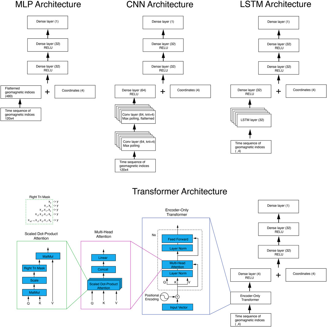
Figure 1. Architectures of MLP, CNN, LSTM and Transformer models for modeling 55 keV ring current proton fluxes, which uses a 10-day history length for geomagnetic indices, and the time sequence length is 120 (2-h cadence). Modeling of >148 keV proton flux uses 40-day history lengths. The term dense layer is also referred to as the fully-connected layer.

3.1 MLP model

Following the work by Li et al. (2023), we establish an MLP network to model ring current proton distributions. The network comprises two hidden layers, each with 32 neurons and followed by a Rectified Linear Unit (ReLU) activation function, the most widely used activation function (e.g., Goodfellow et al., 2016), and a dropout layer (Srivastava et al., 2014) with a rate of 0.2. This architecture and the parameters are chosen after extensive experiments and guided by the evaluation of model performance, specifically, the coefficient of determination R² of the test set.

The lifetime of protons in the ring current region varies significantly depending on energy and L-shell. Our experiments demonstrated that a 10-day historical window of geomagnetic indices is broadly sufficient for predicting 55 keV proton flux. While slightly shorter or longer historical windows may occasionally yield marginally higher R² scores, such improvements are minimal and statistically insignificant due to inherent variability stemming from stochastic processes and initial random settings for weights and biases. Using a 2-h cadence input, we obtain a 120 × 4 matrix for geomagnetic indices (120 time steps, 4 features), which is then flattened into a one-dimensional vector (480 parameters).

For high-energy protons, even though their lifetime is long, our experiments indicate that increasing the historical input length beyond an optimal range (which is shorter than the lifetime) does not consistently enhance performance. This is possibly because increased input dimensionality can introduce detrimental effects such as model overfitting. For proton fluxes at energies above 148 keV with a lifetime of ∼10 s–∼100 s days, we extended the historical input window to 40 days.

3.2 CNN model

In this study, we leverage a CNN to capture spatio-temporal features in geomagnetic indices, treating the N × M as a two-dimensional image. This arrangement allows the CNN to effectively identify characteristic patterns associated with geomagnetic storms and substorm events, as well as how long ago they occurred relative to the data point being predicted. This study employs a 2D-CNN, which captures joint representation across geomagnetic indices. In contrast, using separate 1D-CNN for geomagnetic indices and concatenating their output may miss interactions between indices.

The CNN architecture comprises two convolutional blocks, each followed by max-pooling operations. The first convolutional layer contains 64 kernels, each with dimensions 4 × 4, to extract event patterns from the geomagnetic indices. A max-pooling operation reduces the spatial dimension of the output feature maps. A second convolutional layer, also consisting of 64 4 × 4 kernels, further processes these intermediate feature representations, again followed by max-pooling. The resultant feature maps are flattened and fed into a dense layer of 64 neurons, which are then concatenated with spatial coordinate inputs. Subsequently, two fully connected layers with ReLU activation functions produce the network’s output, modeling the proton flux predictions. We adopted these hyperparameters based on optimization from experiments over a wide range.

3.3 LSTM model

The LSTM network employed in this study consists of 32 recurrent cells designed to process sequential geomagnetic index data recursively. At each time step, these cells generate an encoded representation (a 32-dimensional output vector) that captures essential characteristics of recent geomagnetic activity, such as the magnitude of preceding storm or substorm events and the elapsed time since their occurrence. This temporal encoding is concatenated with four spatial coordinate neurons, resulting in a combined representation of the spatial-temporal context. Subsequently, two fully connected dense layers with ReLU activation functions process this vector to generate predictions of proton flux.

An important advantage of the LSTM model is its flexibility in handling variable-length input sequences without requiring architectural modifications. To capitalize on this feature, we tailored the training strategy according to the proton energy range being modeled. For lower-energy protons (≤148 keV), whose characteristic decay timescales are typically within 10 days, we trained the model using a 10-day historical lookback window of geomagnetic indices. For higher-energy protons (>148 keV), which exhibit substantially longer decay timescales, we utilized a combined training approach, using 40-day, 20-day and 10-day historical windows within each training epoch to update the weights. This methodology ensures robust model performance across varying input sequence lengths, enhancing the consistency and reliability of proton flux predictions.

3.4 Transformer model

This study employs an encoder-only Transformer, corresponding to the encoder part of the original encoder-decoder architecture, to process the sequence of geomagnetic indices. The input layer consists of a vector of geomagnetic indices combined with positional embeddings. Each encoder block follows the design adopted in GPT-3 (Brown et al., 2020), comprising layer normalization (Xiong et al., 2020), a multi-head attention layer with residual connections, a second layer normalization, and a feedforward network with residual connections. We construct the encoder by stacking four such blocks.

At each epoch, the geomagnetic indices are inherently represented as vectors, eliminating the need for the token-to-vector embedding step commonly used in NLP. During training, we considered sequences ranging from a single time step (current geomagnetic indices only) to the full sequence length (120 for <148 keV and 480 for ≥148 keV). To enable parallelization, we applied a triangular mask. Unlike language models that employ a left-triangular mask to autoregressively predict tokens from the beginning of the sequence, our regression model predicts values from any historical window ending at the current step. Therefore, we adopt a right-triangular mask. Finally, because the task is regression rather than classification, we omit the softmax layer typically used in NLP models.

4 Model performance

All models can predict the full proton flux distribution as a function of spatial location and datetime. The MSE between out of sample test-set data and model prediction is an essential metric for evaluating model performance and gives an estimate of the model’s generalizability. Additionally, we also employ the coefficients of determination R² to measure how well the regression predictions approximate the real data points. The R² is defined as

R^{2} = 1 - \frac{\sum_{i} {(z_{i} - y_{i})}^{2}}{\sum_{i} {(z_{i} - \bar{z})}^{2}}

Where z_i is the test data, $\bar{z}$ is the mean value of z_i, and y_i is the model prediction.

We systematically evaluated model performance for proton fluxes at three representative energies. 1) 55 keV, which has a short decay timescale (a few days) across all L-shells and exhibiting strong correlations with geomagnetic indices; 2) 148 keV, having intermediate decay timescales (∼10 days) and responding primarily to moderate and large geomagnetic storms; 3) 269 keV, with significantly longer timescales (>100 days at L = 3.5; Wang and Li, 2023), and predominantly responding only to major geomagnetic storms. We employed all four neural network architectures to model proton fluxes at these representative energies. Figure 2 presents a comparative analysis of each model’s performance, quantified by both MSE and R² correlation between predictions and observational data at each energy. Note that the study by Li et al. (2023) uses averaged fluxes binned to each 0.1 L-shell as the training set, while this study uses 5-min average proton fluxes, allowing for more data samples. Hence, the resultant MLP model performances are notably different.

Figure 2

Twelve scatter plots compare log predicted versus log measured flux for different neural network models (MLP, CNN, LSTM, Transformer) across energy levels (5, 148, 296 keV). Each plot includes a diagonal line indicating perfect prediction, with accompanying R-squared and mean squared error (mse) values. Colors indicate sample density, from blue (few samples) to red (many samples).

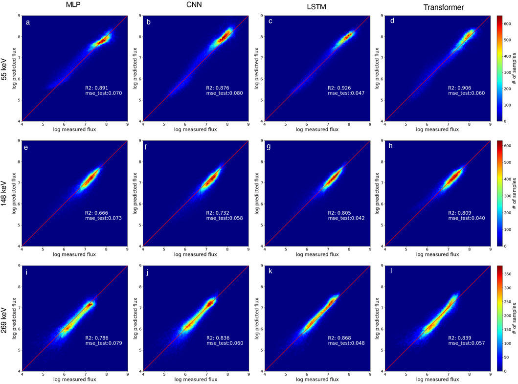
Figure 2. Comparison between test-set proton fluxes and model predictions from the MLP, CNN, LSTM, and Transformer models. Results are presented for three representative proton energies: 55 keV (a–d), 148 keV (e–h), and 269 keV (i–l). Each panel includes the calculated MSE and the coefficient of determination R², quantifying model performance.

Across all examined proton energies, the LSTM and Transformer network consistently demonstrates superior performance compared to the MLP and CNN models, as shown by the lower MSE values and correspondingly higher R² correlations. For all energies, the MSE resulting from the LSTM and Transformer models is smaller than 0.06, which translates to a factor of $10^{\sqrt{0.06}}$ = 1.76, well within the uncertainty range of the measurements. This superior performance of LSTM and Transformer likely stems from their intrinsic capability to effectively process time sequence input data. Moreover, proton flux buildup and decay processes exhibit timescales that vary significantly with L-shell. Unlike the MLP and CNN models, which require a predetermined, fixed-length input sequence, the LSTM and Transformer architectures can flexibly accommodate arbitrary input sequence lengths, both in the training and use phases. This flexibility simplifies model implementation and reduces the redundant work of tuning the input history length for different modeling scenarios.

We note that several sources of randomness may affect neural network training, including the splitting of datasets into training and validation subsets, as well as the random initialization of network weights and biases. Consequently, variations in random seeds may lead to minor differences in model performance metrics, including the test-set MSE and R² scores. Despite this inherent stochasticity, the LSTM and Transformer networks consistently outperform both the MLP and CNN models.

Figures 3a,b illustrate the SME and Sym-H indices throughout the year 2017. Figure 3c shows the observed 55 keV proton flux, and Figures 3d–g show predictions by the MLP, CNN, LSTM, and Transformer models, respectively. All four models give reasonably good performance at this energy, due to their short lifetime, plus a strong correlation between low-energy proton fluxes and geomagnetic indices, even during minor geomagnetic storms.

Figure 3

Time-series graph with six panels: (a) shows SME index fluctuations in nanoTesla; (b) displays SymH index variations; (c) to (g) feature heatmaps labeled Data, MLP, CNN, LSTM, and Transformer, respectively, with color gradients from blue to red. X-axis indicates dates from 02-01 to 12-01, and Y-axis labeled with L values from 3 to 6.

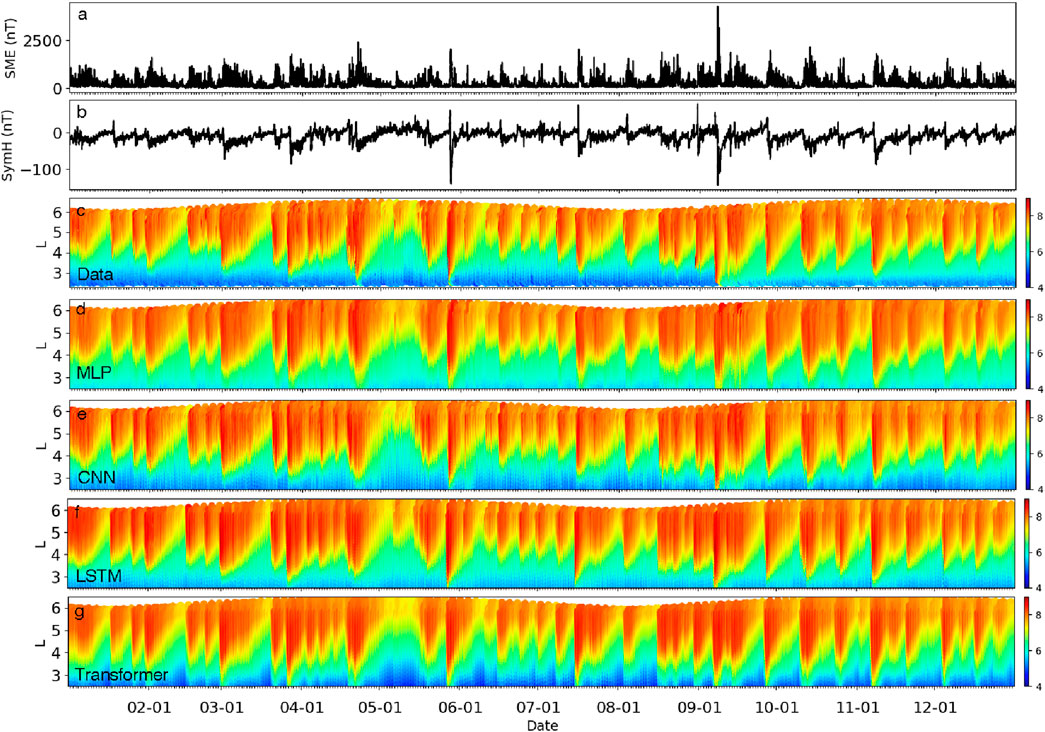
Figure 3. (a) The SME and (b) SymH index over the entire year of 2017 (c–g) The measured 55 keV proton flux of the test set and that predicted by the MLP, CNN, LSTM, and Transformer models, respectively.

Figure 4 shows the observations and model predictions for 148 keV and 269 keV proton fluxes. At the energy of 148 keV, predictions from the MLP model appear notably more erratic, whereas the CNN, LSTM, and Transformer models yield more consistent and stable results. Although the Transformer model achieves the lowest MSE, it underperforms the LSTM in predicting ion dynamics during some small storms. For instance, the observed proton flux shows a depletion during the January 15 storm and an enhancement during the January 31 storm, yet the Transformer model does not show significant changes to these two small storms.

Figure 4

Time series and spectrograms depict solar and geomagnetic data. Panels a and b show SME and Sym-H indices. Panels c to g show 148 keV data modeled by different neural networks (Data, MLP, CNN, LSTM, Transformer). Panels h to l show 268 keV data with the same modeling techniques. The spectrograms use color gradients to represent intensity, ranging from blue (low) to red (high). Dates span from February to December.

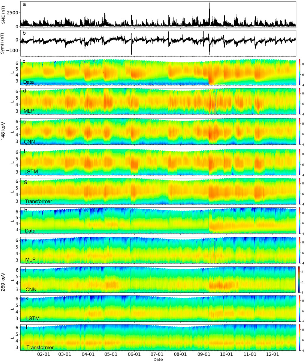
Figure 4. (a) The SME and (b) SymH index over the entire year of 2017. (c–g) The measured 148 keV proton flux of the test set and that predicted by the MLP, CNN, LSTM, and Transformer models, respectively. (h–l) The test set and model predictions for 269 keV proton flux.

The lifetime of high-energy protons at the center of the ring current can extend to several months. We employed a 40-day historical window of geomagnetic indices for modeling proton fluxes at energies of 148 keV and above. Figure 4h shows the observed 269 keV proton flux, and Figures 4i–l present predictions from each model. All models perform well at L shells above L = 4.5, where protons respond to all storms, including minor ones. At low altitudes, the MLP model fails to reproduce the characteristic decay pattern clearly seen in the observational data (Figure 4i), and the CNN model is unable to capture the decay accurately when major storm events occur beyond its 40-day input window (Figure 4j). In contrast, the LSTM model reliably reproduces the prolonged decay behavior, successfully retaining accurate predictions even for events that occurred more than 40 days prior (Figure 4k). The Transformer model predictions (Figure 4l) slightly underestimates storm time fluxes and overestimates quiet time fluxes. This is possibly because the Transformer has a restriction: the total head is equivalent to the number of feature parameters, which is 4 in our case (since we use 4 geomagnetic indices). In contrast, the LSTM model uses 32 cells to remember the current state, which can well record the occurrence of the last large storm and the last minor storm and their intensities.

Predictions from all four models underestimate the acceleration of 148 keV and 269 keV ions following the September 7 geomagnetic storm. Furthermore, the prediction of high-energy proton flux from all four models is not as good as the predictions of low-energy protons. This probably stems from the fact that high-energy protons mainly respond to large storms at low L-shells, but we have insufficient training data covering large storm events, leading to reduced model accuracy in such scenarios. To mitigate the imbalance between abundant quiet-time data and scarce storm-time events, and thereby enhance prediction during major storms, one effective strategy is to apply a customized weighting scheme in the loss function (e.g., Chu et al., 2025).

It is informative to investigate the model’s performance as a function of L shell. Figure 5d illustrates the sample counts of the test set binned to each 0.1 L shell. Due to their elliptical orbit, Van Allen Probes measured more samples around apogee (5.8 Re in geocentric distance) than at perigee. The orbit could be further than L = 5.8 because the spacecraft were sometimes at high magnetic latitudes up to ∼20°. Figures 5a–c illustrate the LSTM model loss for the test set versus L shell at the three selected energies. Impressively, at all these energies, the lowest MSE values occur at L shells where proton fluxes peak and make the most energy contributions to the Dst/Sym-H dynamics (L = 6.3 for 55 keV, L = 4.9 for 148 keV and L = 4.3 for 269 keV), and the lowest MSE values are all within the 0.02–0.025 range. This highlights the strength of machine-learned models–they can accurately capture the most dynamics and significant variations.

Figure 5

Four line graphs labeled a to d, each with different data trends. Graph a shows loss against L with an initial rise, then decline. Graph b shows a U-shaped loss curve. Graph c depicts a V-shaped loss trend. Graph d shows counts peaking sharply near L = 5.5.

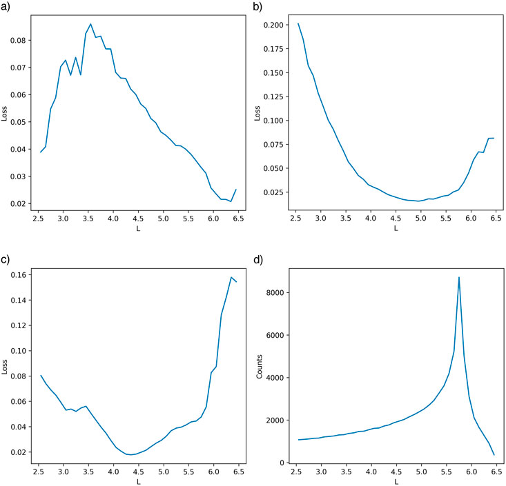
Figure 5. (a–c) The LSTM model loss versus L shell for the test set at 55 keV, 148 keV and 269 keV, respectively. (d) The test set sample counts binned to each 0.1 in L-shell.

5 Discussion

Across all energy levels, the MSE achieved by the models corresponds to prediction errors typically within a factor of two, which is within the uncertainties inherent in the observational measurements. The data from 2013 to 2018 covers half a solar cycle from maximum to minimum. Moreover, the SymH index is proportional to the total energy of the ring current (Dessler and Parker, 1959; Sckopke, 1966), presumably, our model should be applied to the whole solar cycle.

Pires De Lima et al. (2020) experimented with a series of neural networks in making 1-day and 2-day predictions of radiation belt electrons using observations at low Earth orbit, plus the upstreaming solar wind speed as input. Their study shows that the linear regression, MLP, CNN, and LSTM models resulted in similar accuracy, while the linear regression model slightly outperformed other models, probably due to a high linear correlation between precipitation and trapped MeV electrons. Sinha et al. (2021) further showed that nonlinear models outperform linear regression for >2 MeV electrons at L < 4.

In this study, the four models show very close performance for low energy ion fluxes which has a strong correlation with the input, and short-time dependencies. For high-energies, the LSTM and Transformer neural network consistently outperforms the MLP and CNN neural networks, which likely stems from their intrinsic capability to effectively process time sequence input data, especially long sequences (up to 480 in our study). Moreover, proton flux buildup and decay processes exhibit timescales that vary significantly with L-shell. Unlike the MLP and CNN models, which require a predetermined, fixed-length input sequence, the LSTM architecture can flexibly accommodate arbitrary input sequence lengths, both in the training and inference phases. This flexibility simplifies model implementation and reduces the redundant work of tuning the input history length for different modeling scenarios. The LSTM model in our experiments slightly outperforms the Transformer model, possibly because the number of total attention heads is restricted to 4 in this study. This restriction could potentially be overcome by customizing a new Transformer model, for instance, by concatenating two adjacent sequences into one (thus enabling 8 heads). This will be left for future studies.

All models were trained on an NVIDIA RTX 3090 GPU using CUDA. The MLP trained fastest (∼5 s/epoch), while CNN, LSTM, and Transformer models required ∼1 min/epoch. Notably, the Transformer handled all sequence lengths, whereas the LSTM was limited to selected windows (e.g., 10-, 20-, and 40-day for ≥148 keV protons). If training on the same amount of tasks, the Transformer trains faster due to parallelization, whereas the LSTM processes inputs sequentially. On CPUs, however, CNNs, LSTMs, and Transformers incur >10× higher computation time. While model performance could be prioritized over tolerable differences in training time, this may not always apply for large-scale applications. Hence, the MLP model remains efficient for inferences on edge devices, especially for large-scale applications.

6 Conclusion

In this study, we evaluated the performance of four fundamental neural network architectures—the Multilayer Perceptron (MLP), the Convolutional Neural Network (CNN), the Long Short-Term Memory (LSTM) and the Transformer—for modeling ring current proton fluxes using time-sequenced geomagnetic indices as input. The models were trained and tested on proton fluxes at three representative energies: 55 keV, 148 keV, and 269 keV, which s different lifetime and are L-shell-dependent.

Our results show that all four models are capable of learning meaningful patterns and producing reasonable flux predictions. All four models yield accurate prediction for low-energy proton fluxes, and the performances are similar. For modeling high-energy proton fluxes, the LSTM and Transformer networks consistently achieved lower MSE than the MLP and CNN models, demonstrating a stronger ability to capture the long-term evolution of proton fluxes. Besides, both the LSTM and Transformer models offer flexibility by accommodating sequences of varying lengths during both training and inference. The Transformer model slightly underperforms the LSTM model, possibly due to its restriction on the number of output dimension which has to be equal to the input dimension. The LSTM can use any number of cells, making it more-suited for modeling the multi-timescale behavior of ring current ions.

When GPU resources are available, the LSTM and Transformer models are recommended due to their superior accuracy and adaptability. However, the MLP model remains a competitive alternative for CPU-limited or resource-constrained environments, offering a favorable balance between predictive performance and computational efficiency.

Data availability statement

The original contributions presented in the study are included in the article/supplementary material, further inquiries can be directed to the corresponding author.

Author contributions

JL: Conceptualization, Data curation, Formal Analysis, Funding acquisition, Investigation, Methodology, Project administration, Software, Supervision, Visualization, Writing – original draft. JB: Conceptualization, Methodology, Supervision, Writing – review and editing. QuW: Formal Analysis, Investigation, Writing – review and editing. YW: Writing – review and editing, Methodology, Conceptualization. AL: Writing – review and editing, Methodology, Software. MA: Writing – review and editing, Methodology, Software. BW: Writing – review and editing, Methodology. QaW: Formal Analysis, Writing – review and editing, Visualization. JJ: Writing – review and editing, Methodology.

Funding

The author(s) declare that financial support was received for the research and/or publication of this article. JL and JB acknowledge NASA Grants LWS-80NSSC20K0201, 80NSSC21K0522, 80NSSC18K1227, NNX14AI18G, and the Grant DE-SC0010578.

Conflict of interest

The authors declare that the research was conducted in the absence of any commercial or financial relationships that could be construed as a potential conflict of interest.

Generative AI statement

The author(s) declare that no Generative AI was used in the creation of this manuscript.

Any alternative text (alt text) provided alongside figures in this article has been generated by Frontiers with the support of artificial intelligence and reasonable efforts have been made to ensure accuracy, including review by the authors wherever possible. If you identify any issues, please contact us.

Publisher’s note

All claims expressed in this article are solely those of the authors and do not necessarily represent those of their affiliated organizations, or those of the publisher, the editors and the reviewers. Any product that may be evaluated in this article, or claim that may be made by its manufacturer, is not guaranteed or endorsed by the publisher.

References

Abadi, M., Barham, P., Chen, J., Chen, Z., Davis, A., Dean, J., et al. (2016). TensorFlow: a system for large-scale machine learning. arXiv Preprint. doi:10.48550/arXiv.1605.08695