Predicting cutoff L-shells of solar protons using the GPPSn particle dataset

Solar energetic protons (SEPs) arriving at the Earth trigger severe radiation storms in the near-Earth space, directly impacting space missions operating at various altitudes. Therefore, monitoring SEP events and predicting the penetration depths of solar protons are critical for aerospace sectors. Building on previous efforts, here we demonstrate the feasibility of using proton measurements from the Global Prompt Proton Sensor network (GPPSn), enabled by Los Alamos National Laboratory developed combined X-ray dosimeters aboard GPS satellites, to characterize and predict the penetration of solar protons into the geomagnetic field. The inclined medium-Earth-orbits (MEOs) of the global GPS constellation offer a unique advantage of allowing simultaneous measurements of penetrating solar protons inside both open- and closed-field line regions. Therefore, the L-profiles of ∼10s–100 MeV solar protons and their associated cutoff L-shells can be determined from the GPPSn dataset, using predefined threshold proton flux values rather than traditional flux ratios. After examining a list of SEP event intervals across solar cycles 23, 24 and 25—including the 2024 Mother’s Day superstorm, we showcase how the latest GPPSn proton dataset (release v1.10), reprocessed and calibrated, can not only be used to monitor solar proton distributions inside the dynamic geomagnetic field for individual events, but also to derive a new empirical model linking cutoff L-shells with several key space weather parameters. This newly developed SEPCL-MEO model demonstrates high predictive performance; for example, predictions for >30 MeV solar protons yield a correlation coefficient of 0.85 and performance efficiency of 0.67 when validated against GPPSn observations. Results from this pilot study underscores the scientific and operational value of the GPPSn dataset, and this dataset—when paired with machine-learning techniques—can play a critical role in observing and predicting the effects of future incoming SEP events, including extreme ones.

1 Introduction

Bursts of solar energetic particles—primarily originated from solar flares and coronal mass ejections—are a major driver of space weather when they sweep across the Heliosphere. Among various particle species, high fluxes of solar energetic protons (SEPs)—with energies ranging from ∼10s to more than 100 s MeV—present significant space radiation hazards, contributing to both ionizing dose and single event effects. For instance, for interplanetary missions where no intrinsic planetary magnetic field offers protection, SEPs with energies >50 MeV can readily penetrate though nominal spacecraft shielding (Jiggens et al., 2018), causing serious safety risks to astronauts and electronic systems on board (e.g., Sanzari et al., 2014; Tylka et al., 1996).

Solar protons arriving at the Earth can trigger severe radiation storms inside the near-Earth space, directly impacting space missions at high and medium altitudes, and potentially endangering crew members aboard space stations in low-Earth-orbits (LEOs). These protons may also disrupt transpolar flights and, in extreme cases, affect electronics and human health at ground level. In addition to the direct effects, energetic solar protons bombarding the upper atmosphere during major SEP events generate cascades of secondary particles, including neutrons that can pose further risks to airplane passengers and crew flying over polar regions (Wilson et al., 2003). During rare solar cosmic ray events, where solar protons have energies exceeding ∼4-5 hundred MeV or even GeV, the resulting secondary MeV neutrons may reach the ground level at mid-latitude (Shea and Smart, 2000). Such events, known as ground level enhancements (GLEs)—or subGLEs with fewer energetic neutrons—can lead to single event upsets or latch-up failures in both avionics and ground-level microelectronic systems including autonomous vehicles (e.g., Dyer et al., 2006; Cellere et al., 2008). Therefore, monitoring, modeling, and forecasting the SEP events and their terrestrial impacts are of practical significance for a wide range of sectors, particularly in the aerospace industry.

Empowered by Earth’s strong geomagnetic field, the magnetosphere effectively shields our home planet from most SEPs. However, some solar protons can still penetrate to lower altitudes, particularly at high latitudes. One way to access the penetration of solar protons is by specifying their rigidity at a given location: for example, inside the current geomagnetic dipole field, protons reaching the geomagnetic equator at Earth’s surface have a rigidity value of ∼15 GV. In this study, we adopt an alternative approach by examining the minimum L-shells accessible to protons of given energies—referred to as cutoff L-shells. During intense geomagnetic storms or hammered by high-pressure pulses from the upstream solar wind, the near-Earth magnetic field can be weakened or distorted, allowing more solar protons to reach lower latitudes or L-shells. Therefore, accurately predicting SEP cutoff latitudes or L-shells is a critical challenge in space weather research.

While Störmer (1955) provided an analytic solution for cutoffs in a static dipole magnetic field, predicting the cutoffs in Earth’s dynamic magnetospheric environment heavily relies on empirical models. Among them, the Dst-dependent empirical relationship developed by Ogliore et al. (2001) and Leske et al. (2001)—hereinafter referred to as the OL model—is widely used, including in operational tools such as the FAA’s CARI-7A aviation radiation model (Bain et al., 2023). Here Dst refers to the disturbance storm time index (Mayaud, 1980), which measures the intensity of the ring current. A more recent empirical model by van Hazendonk et al. (2022) incorporates a broader set of inputs including solar wind parameters and geomagnetic indices. Despite their value, these models have notable limitations. The OL model has shown significant discrepancies during individual SEP events, often diverging from in-situ observations (e.g., O’Brien et al., 2018; Chen et al., 2020). Furthermore, both the OL and van Hazendonk models use flux ratios, i.e., the ratio of local to upstream proton flux, to define the cutoff locations. This approach is not ideal for practical users, who are typically more concerned with absolute solar proton intensities at a given location rather than a fixed ratio, given the variability of upstream proton flux levels. Therefore, a successful SEP cutoff model should include the time-varying upstream proton intensities as inputs, enabling more accurate and operational-oriented predictions.

Besides existing empirical models, several long-term observational datasets are available for SEP research. Currently, SEPs are routinely monitored by operational satellite missions from NASA and National Oceanic and Atmospheric Administration (NOAA), including solar wind monitors at the Sun-Earth Lagrangian One Point as well as Geostationary Operational Environmental Satellites (GOES) in geosynchronous (GEO) orbit. NOAA’s Polar Operational Environmental Satellites (POES) constellation in LEO also contribute valuable SEP observations, particularly when passing through the high-latitude regions. In addition, NASA’s Van Allen Probes mission (Mauk et al., 2013) provided high-quality observations of energetic protons between 2012 and 2019 in geosynchronous transfer orbits, however with limited SEP events observed during the time including the well-studied September 2017 event (e.g., O’Brien et al., 2018; Qin et al., 2019; Filwett et al., 2020). Another invaluable resource is the Global Prompt Proton Sensor network (GPPSn), which includes GPS satellites along medium-Earth-orbits (MEOs) and was introduced in our previous study (Chen et al., 2020). Making full use of these diverse datasets to improve SEP cutoff prediction is a long-term goal that requires sustained efforts. Here we present the results from an initial demonstrative study focusing on leveraging observations from GEO and GPPSn datasets.

The purpose of this paper is to demonstrate that solar energetic proton cutoff L-shells can be reliably predicted using new empirical relationships derived from GPPSn observations in MEOs. This new model, named SEPCL-MEO hereinafter, is driven by inputs including solar proton intensities measured at ∼ GEO, and is shown to predict cutoff L-shells—defined by predefined threshold flux values rather than flux ratios—with consistent accuracy. This paper is structured as follows: Section 2 describes the observational datasets and the L-profile fitting method used in this study. Section 3 details the training and validation of this new empirical model, along with quantitative performance metrics. Section 4 discusses model limitations and future directions, and Section 5 provides a summary of key findings and conclusions.

2 Datasets, cross-calibration, and fitting methodology

GPPSn observations over selected time intervals are used in this study to derive L-profiles and identify cutoff L-shells of penetrating solar protons. Detailed descriptions of GPPSn dataset can be found in Chen et al. (2020) and Morley et al. (2025); a brief recap is provided here. Since 2000, dozens of GPS satellites have carried particle instruments developed by Los Alamos National Laboratory to measure in-situ electrons and protons in circular MEOs at a nominal altitude of ∼20,200 km and an inclination of 55°. The onboard Combined X-ray Dosimeter (CXD) instrument (Tuszewski et al., 2004) measures protons with energies from ∼6 MeV up to greater than 75 MeV in both closed- and open-field line regions at L-shells above ∼4. The latest data release, version 1.10, provides proton differential and integral fluxes from 10–10⁴ MeV with a time resolution of 4 min spanning from 2000 to 2024. This dataset uses the response functions and calibration factors established by Carver et al. (2018). The data are archived at https://www.ngdc.noaa.gov/stp/space-weather/satellite-data/satellite-systems/lanl_gps/version_v1.10r1/. Readers are referred to Morley et al. (2017); Carver et al. (2018) and Morley et al. (2025) for further details on the data generation and preparation. To avoid confusion, we refer to the collection of further-calibrated GPS proton data, treated as a unified source, as the GPPSn dataset. Based on prior calibration results by Carver et al. (2018) and Chen et al. (2020) as well as considerations of energy-dependent penetration depths, GPSSn data used in this study are limited to integral proton fluxes for four energy thresholds >20, >30, >50, and >80 MeV, to ensure data quality.

For this demonstrative study, we also use the solar energetic particle environment modeling (SEPEM) dataset in place of original GOES proton measurements, taking advantage of the extensive efforts described by Crosby et al. (2015). The SEPEM reference proton data set was constructed using measurements from multiple proton instruments aboard a list of GOES satellites and the Interplanetary Monitoring Platform 8 (IMP 8). The dataset was developed through systematic processing steps involving data cleaning, gap filling, energy rebinning, and cross-calibration. SEPEM dataset v2.00 is used here, covering from 1974 to 2015 and including 11 reference energy channels exponentially spaced from six to above 200 MeV with a 5-min time resolution. Here, SEPEM dataset is treated as the gold standard, and is used for both verifying/improving the calibration of GPPSn dataset and, where available, as a source of model inputs at GEO.

For this initial study, we selected twelve solar proton event intervals from NOAA’s Solar Proton Events list (https://umbra.nascom.nasa.gov/SEP/), focusing on major events with significant >10 MeV proton flux unit (pfu) values falling within GPSSn dataset’s time coverage. As summarized in Table 1, a subset of six intervals—intervals 1, 2, 6, 7, 8, and 10—is used for developing and training heuristic relationships, while the remaining six intervals are reserved for validating model performance. Note each interval in Table 1 may include multiple SEP events, geomagnetic storms, and GLEs. Care was taken to ensure that both subsets span the full range of geomagnetic storm intensities, providing representative coverage for model development and evaluation.

Table 1

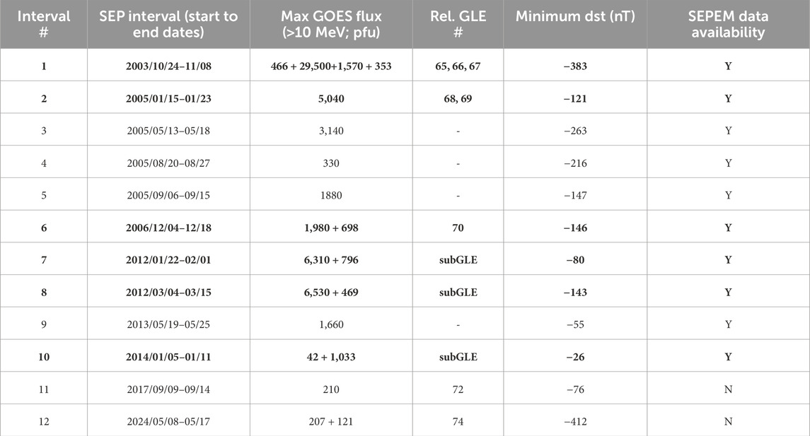
Table 1. List of 12 selected solar energetic particle (SEP) event intervals. Columns include: interval number, start and end dates, peak proton flux unit (pfu) value for >10 MeV protons in individual SEP events, associated GLE/subGLE events, minimum Dst value during the interval, and SEPEM data availability for cross-calibration with GPPSn fluxes. Six intervals—1, 2, 6, 7, 8, and 10 (bolded rows)—are used for model development/training in this study, while the remaining six intervals—3, 4, 5, 9, 11, and 12—are reserved for out-of-sample model validation.

Cross-calibration of GPS proton fluxes against SEPEM fluxes is a critical step in this study. Although the following L-profile fitting process uses only normalized fluxes, the determined cutoff L-shell locations used for model validation will depend on the absolute flux values from the GPPSn dataset. While cross-calibration between GPS and GOES proton fluxes were performed prior to each public release of the GPS particle dataset (Morley et al., 2025, and references therein), we further compare GPS fluxes with SEPEM fluxes to confirm and fine-tune the calibration within each SPE interval. One such example is shown in Figure 1 for Interval 7. In both panels, proton fluxes measured in the open-field line region (L > 9) by ten GPS satellites over 11 days are compared with simultaneous SEPEM fluxes at >30 and >80 MeV. The data points are seen to cluster tightly around the diagonal lines, representing a close alignment, and their spreads are well contained within the two dashed lines indicating flux deviation factors of 1.5 and (1/1.5). In addition, power-law fitting functions for the ten GPS satellites—this number differs for different intervals—are provided on the right-side of the panels, with all coefficients very close to unity, further confirming good agreement. Similar results were obtained for other energies and SEP intervals, with additional examples in the Supplement. By applying these derived fitting functions to the fluxes from each GPS satellite, we have a uniformly calibrated GPPSn fluxes for subsequent analysis. In the following steps, all GPPSn fluxes are averaged over 2-h and 0.2 L-shell bins.

Figure 1

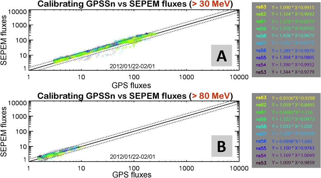
Figure 1. Cross-calibrations between GPS and SEPEM proton fluxes in open-field line regions during Interval 7 (January 2012). Two panels correspond to two energies: >30 MeV in panel (A) and >80 MeV in panel (B). In each panel, proton fluxes from ten GPS satellites (color-coded) are compared to simultaneous SEPEM fluxes over this 11-day interval, binned to the same 5-min time resolution. The solid diagonal represents perfect calibration, whereas the dashed lines on both sides indicate upper and lower deviation factors of 1.5 and (1/1.5), respectively. Linear regression fitting functions—using GPS fluxes as inputs X to best match SEPEM fluxes Y—are shown to the right of each panel, with colors matching the corresponding GPS satellites.

To identify cutoff L-shells from the GPPSn dataset, we apply the Weibull cumulative distribution function to fit the L-profile of normalized fluxes. That is, in each 2-h time bin, GPPSn fluxes j(L) in the closed-field line region are normalized to $j\left(\infty \right)$, the flux in open-field line regions. The derived L-profile is then fitted using the Weibull function:

$\mathit{F}\left(\mathit{L}\right)=\frac{\mathit{j}\left(\mathit{L}\right)}{\mathit{j}\left(\mathit{\infty }\right)}=\mathbf{1}-{\mathit{e}}^{\left[-{\left(\frac{\mathit{L}}{{\mathit{L}}_{\mathbf{0}}}\right)}^{\mathit{\gamma }}\right]}(1)$

where L₀ is the scale parameter (usually different from the cutoff L-shell) and γ is the shape parameter. This fitting determines the functional form of F(L) describing the transition of solar protons from open-to closed-field line regions. Figure 2 shows several example Weibull curves, simulating solar protons penetrating from high L-shells with typical (L₀, γ) values obtained in this study. It illustrates that the L₀ parameter sets the L location at which flux ratios drop to 0.632, while the γ parameter together with L₀ controls the width and steepness of the cliff-like portion. By comparing these curves in Figure 2, we gain insight into the relative sensitivity of cutoffs to the two parameters. For example, using a threshold flux ratio of 0.2, the solid red curve for (L₀ = 5, γ = 15) gives a cutoff L-shell at ∼4.5. If L₀ increases by 20% to 6 but keeping the same γ, the blue curve shows a cutoff at ∼5.4. Conversely, reducing γ by 33% to 10 but keeping the same L₀, the red dot-dashed curve yields a cutoff at ∼4.3. These examples suggest that cutoff locations are more sensitive to changes in L₀ than in γ. Indeed, this is further supported by the total differential of Equation 1, which indicates that for typical (L₀, γ) values in this study, this fitting’s sensitivity to L₀ is about five times greater than to γ. Given a Weibull curve characterized by fitted (L₀, γ) parameters, together with the known upstream solar proton flux, one can use Equation 1 to determine the cutoff L-shell corresponding to any specified threshold proton flux value.

Figure 2

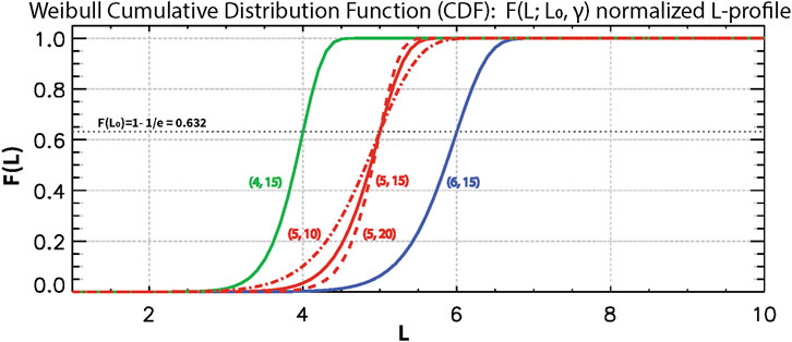
Figure 2. Example Weibull cumulative distribution function (CDF) curves for five different parameter combinations of (L₀, γ). Each curve is normalized such that F(L) = 1 at large L-shells (L > 9), representing to the open-field line region, and then F(L) drops to zero with a cliff-like slope to simulate the normalized spatial flux profile of penetrating solar protons. The parameter L₀ defines the L-shell where all F(L) = 0.632, while the parameter γ determines the steepness of the transition.

Weibull fitting has been successfully applied in previous studies, e.g., O’Brien et al. (2018) and Chen et al. (2020), and its use in this study offers several advantages. First, it enables extrapolation into L-shells below 4, where GPPSn data are unavailable. Second, it helps to minimize the contamination from MeV electrons sometimes affecting L∼4 and above (Chen et al., 2021). Most importantly, the fitting reduces observations in each time bin to two key parameters—L₀ and γ—for model development. Our new predictive model includes two internal steps: One to predict the Weibull parameters (L₀, γ) to reconstruct the full L-profile of solar protons, and two to determine the cutoff L location for given threshold flux values. This two-step approach preserves the flexibility to vary threshold flux levels compared to directly predict the cutoff locations.

For the hundreds of solar proton L-profiles analyzed across all energies from >20 MeV to >80 MeV, non-linear least squares fitting using the Levenberg-Marquardt algorithm yielded mean relative fitting error percentages ranging from 10% to 13% when averaged over all L-shells, and from 7% to 20% when averaged specifically over the L-shells between 4 and 6, where solar proton flux drops most sharply. To ensure robust fitting and reliable determination of cutoff L-shells, we applied these selection criteria to each selected time bin: both the mean relative fitting error percentages over all L-shells as well as over [4, 6] must be below 30%, and the set of fitted data points must include at least one value where the normalized flux ratio drops to 0.75 or lower, in order to avoid excessive extrapolation. Following these criteria, the Weibull fitting produced reasonably good results: more than 80% of all time bins were deemed usable for model development and validation, with their mean fitting error percentages below 9.5% over all L-shells and below 14% at L-shells within the critical L = 4 – 6 range.

Figure 3 presents example results for Interval 7 from the analysis steps described above. The top panel A shows >30 MeV proton fluxes from SEPEM (in black) compared with fluxes from ten GPS satellites (color-coded) in open-field line regions, after applying the calibration functions presented in Figure 1A. Besides the overall agreement between GPS and SEPEM fluxes, the several outliner data points from satellite ns61 between 36 and 48 h are effectively washed away by consistent observations from other GPS satellites—highlighting the advantage of using multi-satellite observations. Panel B shows the binned GPPSn fluxes—without interpolation or extrapolation—as a function of L-shell and time with two SEP events. Here the white line represents cutoff L-shells from the OL model, while the yellow points indicate the cutoffs determined from GPPSn flux L-profiles using a threshold flux value of 3 pfu. Bottom Panels C–E show three example moments in which the red squares denote the cutoffs determined via Weibull fitting, which closely overlap with the blue points derived from direct interpolation of GPPSn fluxes. This process is repeated for the six training intervals to derive (L₀, γ) values for the statistical analysis and model development, and also to all 12 intervals to determine the cutoff L-shells that serve as ground truth to quantify performance of the new SEPCL-MEO model.

Figure 3

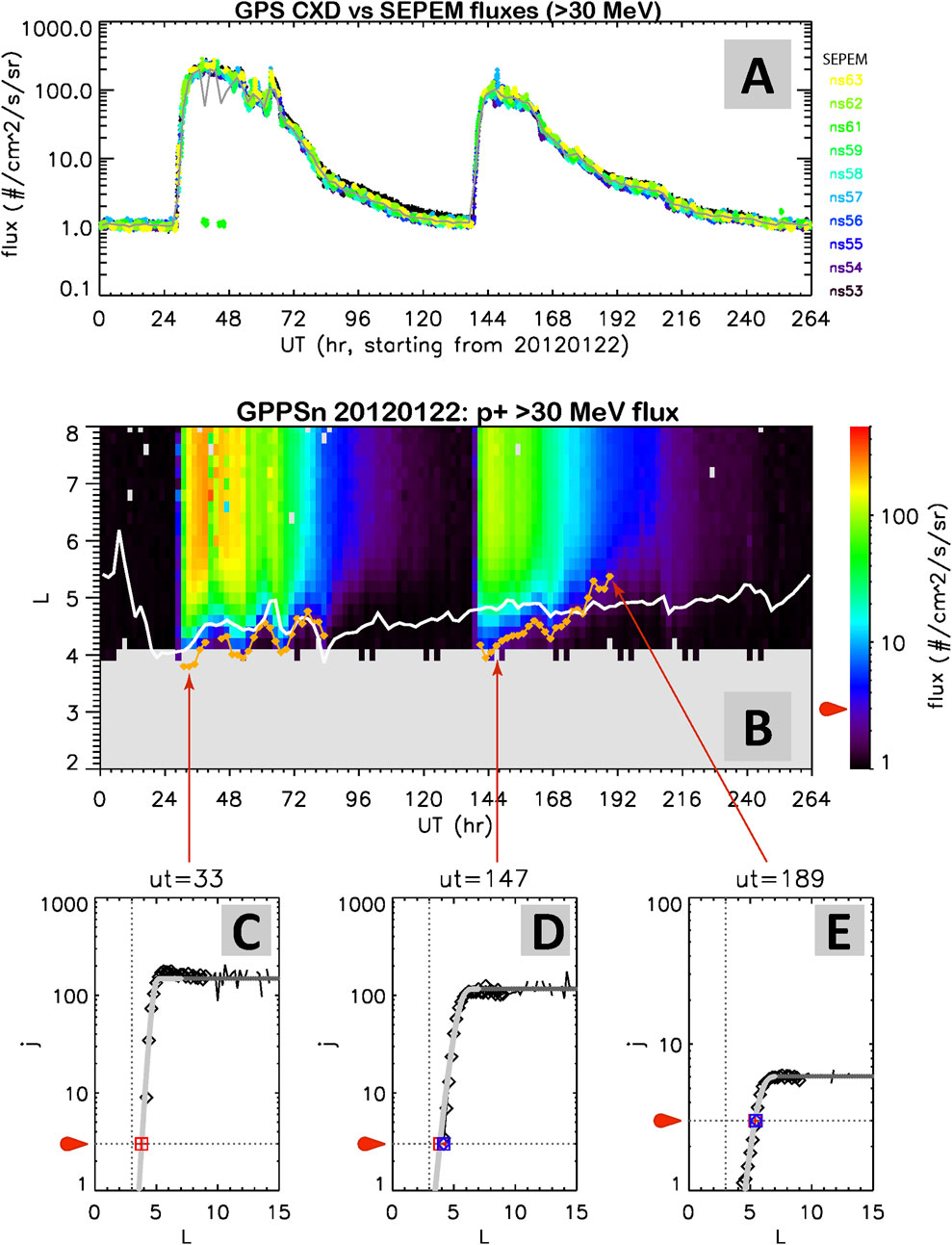
Figure 3. Example results from Interval 7. (A) SEPEM fluxes (black) are compared with calibrated GPS fluxes (color-coded by satellite) in the open-field line region for >30 MeV protons over 11 days. The gray curve shows 2-hourly binned GPPSn fluxes, averaged across all 10 GPS satellites. (B) GPPSn fluxes for >30 MeV protons, binned by 2 h and 0.2 L-shell, are shown as a function of time and L-shell. The white curve plots cutoff L-shells from the OL model, and yellow data points represent cutoff L-shells identified via Weibull fitting. (C–E) Examples of observed flux L-profiles (black data points) compared with fitted Weibull curves (gray lines) at three selected times. Cutoff L-shells are identified using two methods: red symbols from Weibull fitting and blue symbols from direct interpolation of the observed points (where possible). Vertical dashed lines mark L = 4, while red arrows and horizontal dashed lines indicate the predetermined threshold flux of three particles/cm²/s/sr for >30 MeV solar protons. Note that all flux data pointes shown in Panels (B–E) are directly binned from GPPSn data, without any interpolation or extrapolation.

3 Model development and performance evaluation

With all (L₀, γ) values derived from the six training intervals, our next step in developing the SEPCL-MEO model is to select and construct the appropriate input parameters. This is carried out in a heuristic manner, guided by both physical insights and trial-and-error testing. For each time bin, the model first predicts L₀, followed by γ determination. L₀ is known to be correlated with geomagnetic activity levels. For example, the OL model uses the Dst index, while van Hazendonk et al. (2022) demonstrates the importance of solar wind flow pressure. Given the known influences from both parameters to cutoffs, we tested various combinations of Dst and solar wind flow pressure P_sw. After extensive tests, we adopted the following heuristic formulation for the input parameter X_scale:

${\mathit{X}}_{\mathit{s}\mathit{c}\mathit{a}\mathit{l}\mathit{e}}=\mathit{D}\mathit{s}\mathit{t}-\mathbf{50}*{\mathit{log}}_{\mathbf{10}}\left({\mathit{P}}_{\mathit{S}\mathit{W}}\right)(2)$

where both Dst (in the unit of nT) and P_SW (nPa) are averaged over the current 2-h bin. As shown in Figure 4A (using the example of >20 MeV protons), data-derived L₀ values from all six training intervals exhibit a Spearman correlation—measuring monotonic but not necessarily linear relationships—coefficient value of 0.77 with X_scale, which is considered high for this study. The general trend in Figure 4A shows that L₀ decreases with decreasing X_scale, reflecting the expected physical picture of a compressed geomagnetic field during storms or under high upstream solar wind pressures. The decreasing trend in L₀ appears to “saturate” for very negative X_scale values. Therefore, to capture this behavior, we applied a two-segment linear fit, separated with breakpoint at X_scale = −130 as identified from the data distribution in Panel A, and fitted each segment using least-squares. The two linear fittings are then smoothly connected using weight functions W_L and W_R, and the full fitting function form for predict L₀ is like:

${\mathit{L}}_{\mathbf{0}}\left({\mathit{X}}_{\mathit{s}\mathit{c}\mathit{a}\mathit{l}\mathit{e}}\right)=\left({\mathit{a}}_{\mathit{L}}+{\mathit{b}}_{\mathit{L}}*{\mathit{X}}_{\mathit{s}\mathit{c}\mathit{a}\mathit{l}\mathit{e}}\right)*{\mathit{W}}_{\mathit{L}}+\left({\mathit{a}}_{\mathit{R}}+{\mathit{b}}_{\mathit{R}}*{\mathit{X}}_{\mathit{s}\mathit{c}\mathit{a}\mathit{l}\mathit{e}}\right)*{\mathit{W}}_{\mathit{R}}(3)$

where the weight functions are both Weibull functions defined as ${\mathit{W}}_{\mathit{R}}=\mathit{F}\left({\mathit{L}}_{\mathbf{0}}=-\mathbf{130},\mathit{\gamma }=\mathbf{50}\right)$ for the right branch and ${\mathit{W}}_{\mathit{L}}=\mathbf{1}-{\mathit{W}}_{\mathit{R}}$ for the left. With the coefficient values determined (listed in the top row of Table 2), the red curve in Figure 4A shows the fitted L₀ values for >20 MeV protons.

Figure 4

Figure 4. Results from SEPCL-MEO model development. (A) For >20 MeV protons, L₀ values determined from GPPSn data over six training intervals are plotted in black as a function of the input parameter X_scale. The red curve shows the fitted function, with the fitting equation provided. (B) γ values determined from GPPSn data over six training intervals are plotted in black as a function of the input parameter X_shape. A linear fit is overplotted in red, with the corresponding equation provided. (C) Cutoff L-shell values predicted by SEPCL-MEO model compared to those from GPPSn observations for >20 MeV protons, yielding a correlation coefficient (CC) value of 0.90. (D) Cutoff L-shells from the OL model compared to GPPSn results, showing a CC value of 0.41. (E,F) Color-coded fitting curves for all four proton energy ranges that will be used by SEPCL-MEO model.

Table 2

Table 2. Coefficients for the SEPCL-MEO model as determined for Equations 3, 5.

The input parameter used to predict the γ value was constructed in a similar way. Initial analysis revealed a significant negative correlation between γ and L₀ values derived from GPPSn data. In addition, we identified the correlations between γ to the energy spectrum of upstream solar wind protons and to Dst. Based on extensive tests, we defined the input parameter X_shape as:

${\mathit{X}}_{\mathit{s}\mathit{h}\mathit{a}\mathit{p}\mathit{e}}={\left({\mathit{L}}_{\mathbf{0}}\right)}^{\mathbf{2}}–\mathbf{0.65}*{\left({\mathit{\alpha }}_{\mathit{p}}\right)}^{\mathbf{2}}-\mathbf{0.05}*\mathit{D}\mathit{s}\mathit{t}(4)$

where L₀ is the predicted value from Equation 3, and α_p is the energy spectral index of upstream solar protons, obtained from SEPEM fluxes or measurements at ∼ GEO. Both α_p and Dst are averaged over the corresponding 2-h time bin. In Figure 4B, the γ values derived for >20 MeV protons from GPPSn dataset are plotted against X_shape. The Spearman correlation has a value of −0.42, which is deemed acceptable given the lower sensitivity of the Weibull function to γ (as discussed in Section 2). We then use a simple linear fit to model γ with the input X_shape:

$\mathbf{\gamma }\left({\mathit{X}}_{\mathit{s}\mathit{h}\mathit{a}\mathit{p}\mathit{e}}\right)=\mathit{c}+\mathit{d}*{\mathit{X}}_{\mathit{s}\mathit{h}\mathit{a}\mathit{p}\mathit{e}}(5)$

Using the least-squares fitting approach, we derived the values of coefficients c and d, as in the top row of Table 2, and the fitting line is shown in red in Figure 4B.

Using the predicted (L₀, γ) values from Equations 3, 5, along with upstream solar proton fluxes from the SEPEM dataset, the SEPCL-MEO model can predict cutoff L-shells for >20 MeV protons across the six training intervals. These model predictions show strong agreement with the cutoff L-shells determined from GPPSn dataset, with a high linear Pearson correlation coefficient (CC) value of 0.90, as shown in Figure 4C. For comparison, cutoff predictions from the OL model are plotted against GPPSn results in the same format in Figure 4D, with a lower CC value of 0.41. For the four distributions shown in Panels A–D, their p-values are all extremely small, less than 10⁻¹¹, indicating strong statistical significance and thus supporting rejection of the null hypothesis.

By applying the procedure described above to all four energies, we developed the complete SEPCL-MEO model using the input parameters defined in Equations 2, 4, with all fitting coefficient values for predicting (L₀, γ) listed in Table 2. The corresponding fitting curves are also plotted in Figures 4E,F. In Figure 4E, for a given X_scale value, higher-energy protons have smaller L₀ values, suggesting deeper penetration into the magnetosphere as expected. Note in Table 2 for >80 MeV, due to a lack of data points at X_scale <∼-250, we assume a flat slope (i.e., b_L = 0) for the left segment fitting, considering b_L values for other energies are all very close to zero. The lack of observations may also account for the changing trend of the fitting curve for >80 MeV in Figure 4F.

Predictions from the SEPCL-MEO and OL models were visually inspected and compared against GPPSn observations to evaluate the accuracy. Figures 5, 6 first present results over four intervals used for model development (i.e., in-sample intervals). The left panels in Figure 5 are for Interval 10, which includes two SEP events under minimal geomagnetic disturbance. In this case, the cutoff L-shells predicted by the SEPCL-MEO model, which increase with receding upstream solar proton intensities, closely match the cutoffs from GPPSn observations. In contrast, predictions from the OL model, which rely solely on the Dst index, show limited dynamics. The right panels in Figure 5 show Interval 7, which contains two consecutive moderate geomagnetic storms and two SEP events. Again, SEPCL-MEO predictions align with GSSPn data well, capturing variations driven by both Dst and upstream solar proton fluxes. In Figure 6, the left panels display Interval 2, which includes two SEP peaks during a period of intensive storms. Here predictions from our new model generally agree with observations but show noticeable overestimates, particularly following the first solar wind high pressure pulse on January 18. The gap in P_sw data on January 20 prevents SEPCL-MEO model to generate predications. (This date coincides with GLE 69 that is the second most intense event ever recorded.) The right panels of Figure 6 show Interval 1 that includes a super geomagnetic storm with a minimum Dst reaching −383 nT. (In this study, superstorms are loosely defined as events with a minimum Dst < −350 nT, representing a small subset of the extreme storms with minimum Dst < −250 nT) The gap in P_sw data on October 30 again prevents SEPCL-MEO model from making predictions over the two Dst dips in the main phase, but at other times SEPCL-MEO results agree with GPPSn observations reasonably well. Therefore, the SEPCL-MEO model shows high performance over these in-sample intervals.

Figure 5

Figure 5. Results from applying the SEPCL-MEO model to two in-sample SEP intervals. Panels in the left column are for one near-quiet period (Interval 10), while those in the right column represent Interval 7 which includes a moderate geomagnetic storm. In each flux panel, red data points connected by black lines show cutoff L-shells predicted by the SEPCL-MEO model; white line plots cutoffs from the OL model; and yellow data points indicate cutoffs directly determined from GPPSn observations. The vertical color bar indicates proton fluxes in the unit of #/cm^2/s/sr, and the red arrow on the left side marks the threshold flux value for the corresponding proton energy. Middle-row panels show the Dst index (black) and solar wind flow pressure P_sw (gray). The start and end of related subGLE events are indicated by yellow bars at the top of the middle panels.

Figure 6

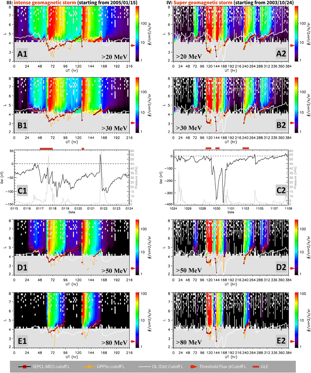
Figure 6. Results from applying the SEPCL-MEO model to two additional in-sample SEP intervals. Panels in the left column are for Interval 2 with intense geomagnetic storms, while those in the right column represent Interval 1 featuring a super geomagnetic storm. All panels follow the same format as Figure 5. The start and end of associated GLE events are indicated by red bars at the top of the middle-row panels.

Predictions from the SEPCL-MEO and OL models were also visually inspected and compared against GPPSn observations over four validation (i.e., out-of-sample) intervals, selected to represent the same geomagnetic disturbance levels. For the near-quiet Interval 9 as in the left panels of Figure 7, the SEPCL-MEO model again shows strong agreement with GPPSn observations, similar to the in-sample results. In the right panels, the SEPCL-MEO model tends to overestimate cutoff L-shells for the moderate Interval 9 but still captures the overall temporal trend. An overestimate from the SEPCL-MEO model is also observed during the intense storm as in the left panels of Figure 8. However, the model performs quite well during the main phase of the 2024 Mother’s Day superstorm (right panels of Figure 8), almost accurately reproducing the observed cutoff L-shells. In contrast, the OL model severely underestimates the cutoffs in this case, with values dropping below L = 2, much lower than observations. Overall, the SEPCL-MEO model demonstrates qualitatively comparable performance on these out-of-sample intervals, confirming its ability to generalize beyond the training set and to varying space weather and geomagnetic conditions.

Figure 7

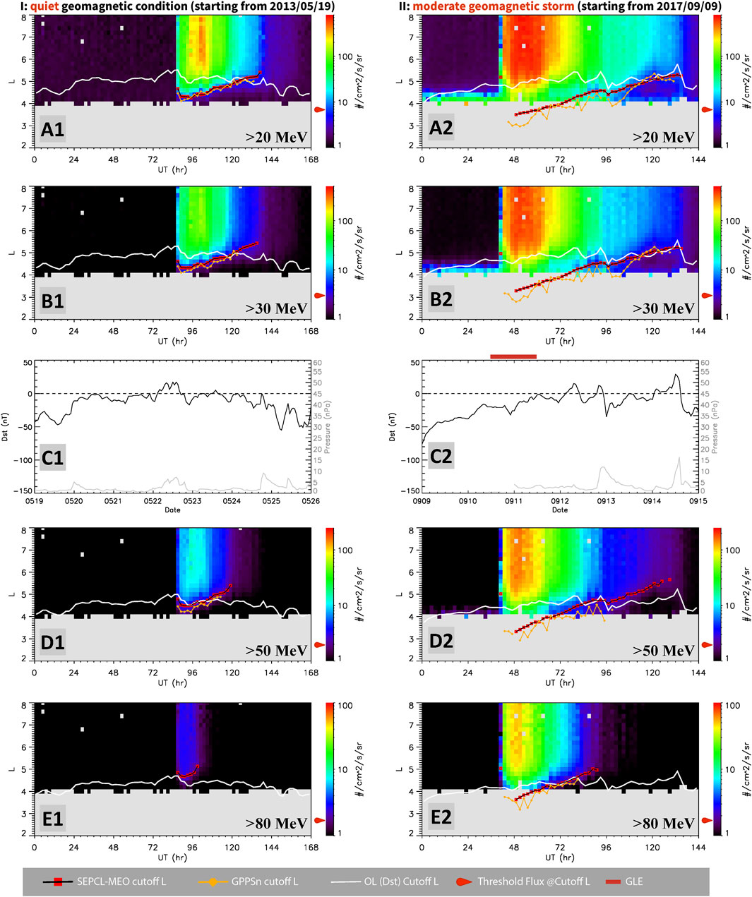
Figure 7. Results from applying the SEPCL-MEO model to two out-of-sample SEP intervals. Panels in the left column are for one near-quiet period (Interval 9), and those in the right column represent Interval 11 which occurs in the recovery phase of a moderate geomagnetic storm. All panels follow the same format as Figure 6.

Figure 8

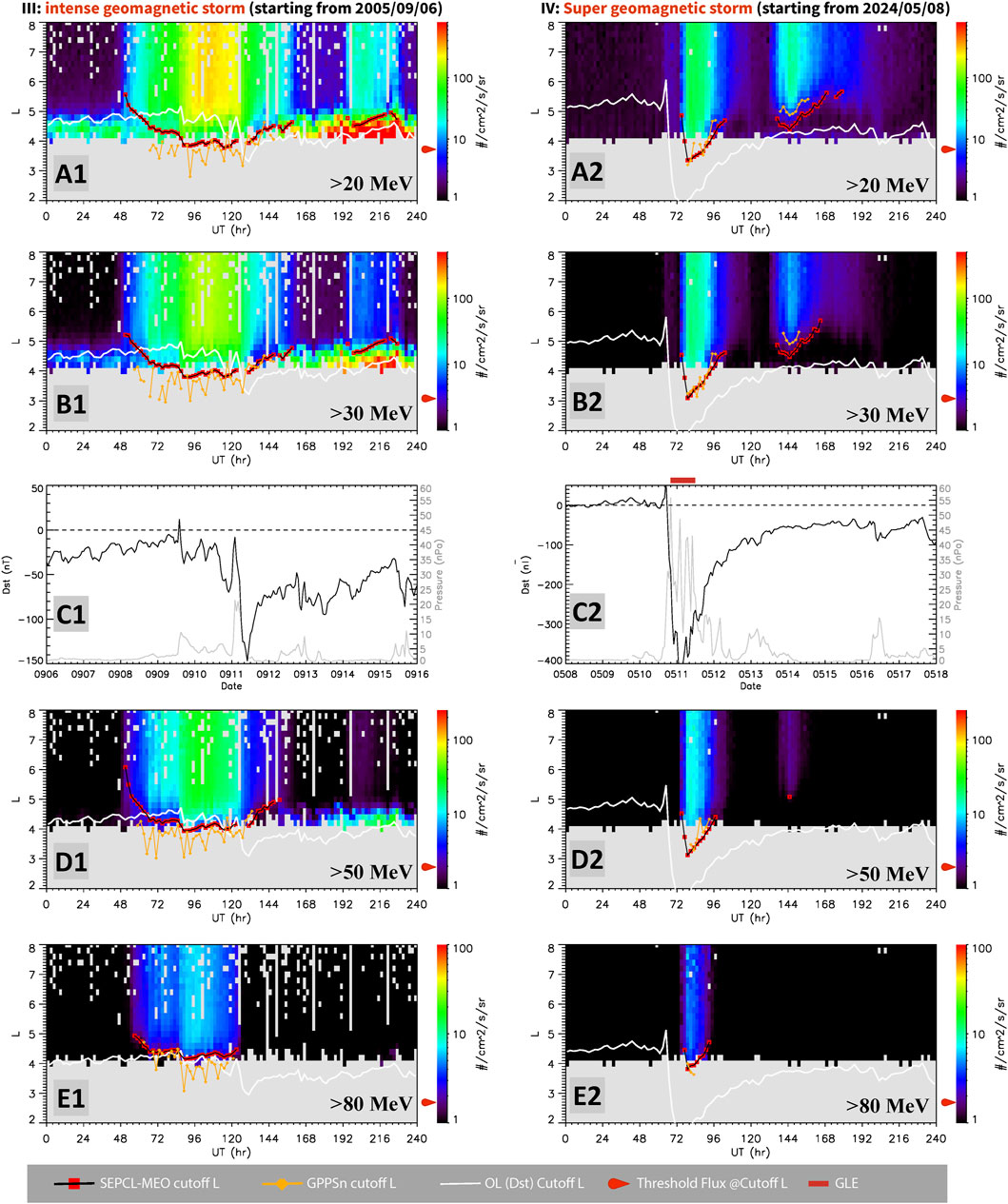
Figure 8. Results from applying the SEPCL-MEO model to two additional out-of-sample SEP intervals. Panels in the left column are for Interval 5 with an intense geomagnetic storm, while those in the right column represent Interval 12 featuring the Mother’s Day super geomagnetic storm in 2024. All panels follow the same format as Figure 6. Contaminations from MeV electrons at L-shells ∼4 – 5 on the last two days are visible in left panels.

Quantitative performance metrics for the SEPCL-MEO model are summarized in the left half of Table 3, compared to corresponding values for the OL model shown in the right. The high performance of SEPCL-MEO is evident across all metrics. For instance, with >30 MeV protons, SEPCL-MEO achieves a CC value of 0.88 and a performance efficiency (PE) of 0.74 for the six training intervals, and a CC value of 0.80 and PE value of 0.49 for the six validation intervals (Here PE is defined following Feng et al. (2024) with preferred values larger than 0 for high skill and one represents perfect.). All these values are significantly higher than those for the OL model: CC = 0.29 for training intervals and CC = 0.20 for validation, and negative PE values for both. Among all proton energies, the SEPCL-MEO model has the best performance for >20 MeV protons, with performance gradually degrading as energy increases. The lowest performance is for >80 MeV protons: CC = 0.68 and PE ∼0 for training, and CC = 0.65 for validation with no PE calculated due to limited available observations. In terms of prediction errors in cutoff L-shell values, SEPCL-MEO yields a mean error value close to zero for all energies except for >80 MeV, and standard deviations ranging from 0.28–0.40—again significantly smaller than those for the OL model. The mean absolute deviations (MAD) of the SEPCL-MEO model range from 0.19–0.31 and the 95th percentile absolute difference values fall between 0.47 and 0.85, while OL model has mean absolute differences ranging from 0.42–0.84 and 95th percentile values within 1.0–1.7. Collectively, all metrics presented in Table 3 demonstrate the outperformance of the SEPCL-MEO model. However, it is important to note that this comparison is not strictly “apples-to-apples”. The OL model makes predictions based on a fixed solar proton flux ratio, whereas SEPCL-MEO predict cutoffs for pre-determined threshold proton flux values. From practical users’ perspective, this distinction matters—misapplying the OL model may result in significantly larger errors when estimating cutoffs to a deemed safe proton level. In this study, to balance practical considerations and observational coverage, the threshold flux levels for determining cutoffs are empirically set to 6, 3, 2, and 1.5 pfu for the four energy values from lowest to highest, respectively.

Table 3

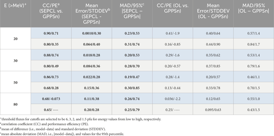
Table 3. Model performance metrics for the SEPCL-MEO and OL models. Columns include: CC and performance efficiency (PE), mean model error and the standard deviation, as well as mean absolution deviation (MAD) along with the 95th percentile deviation. Left half of the Table shows performance metrics for the SEPCL-MEO model, and the right half for the OL model. For each proton energy range, the top row with blue background corresponds to model performance over training intervals, while the bottom row with gray background represents performance over validation intervals.

As an adaptational illustration, Figure 9 presents detailed error distributions of the two models for >30 MeV solar protons. Panel A shows that SEPCL-MEO predictions has narrow error distributions, with a mean deviation of approximately 0.02 across all 12 SEP intervals—indicating a strong match with GPPSn observations. In comparison, Panel C suggests that the OL model tends to consistently overestimate cutoff L-shells, resulting a mean deviation value ∼0.37 and a flatter error distribution. In terms of absolute differences in Panels B and D, SEPCL-MEO model yields a MAD value of 0.24 and a 95th percentile value of 0.63, while OL model has a MAD value of 0.63 and a 95th percentile value > 1.5. These clearly confirm that SEPCL-MEO outperforms the OL model across all selected 12 SEP intervals. Additionally, the error distributions in Figure 9 show the similar shapes for training, validation, and combined intervals, which further confirms the consistency and robustness of the high performance of the SEPCL-MEO model for all conditions. Similar results were found for other proton energies, with additional examples provided in Supplement.

Figure 9

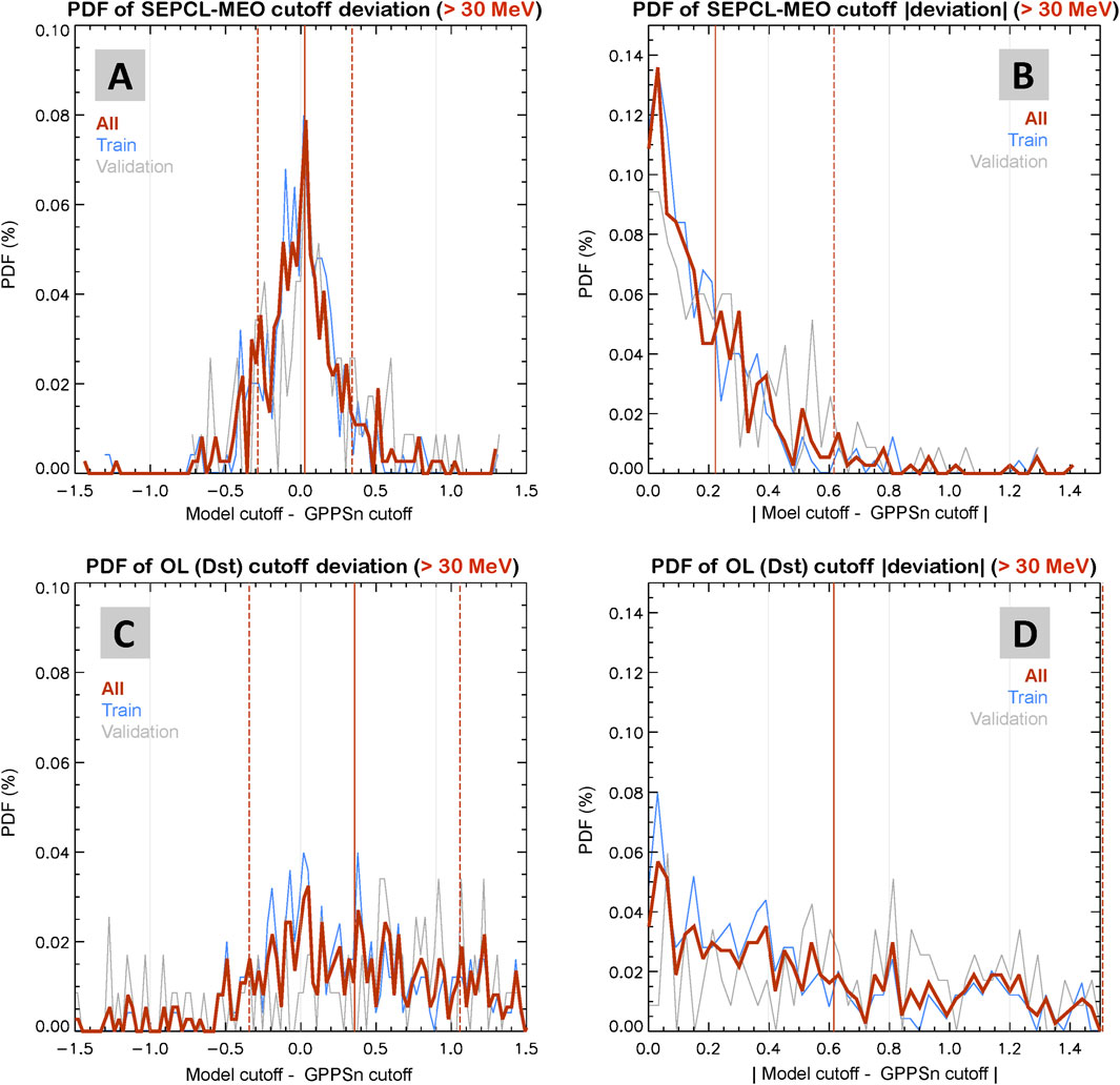
Figure 9. Statistical distributions of prediction errors for the SEPCL-MEO and OL models on >30 MeV solar protons. (A) Probability density functions (PDFs) of SEPCL-MEO model error, defined as the difference between predicted cutoff L-shells and GPPSn-derived values. Blue, gray, and red curves represent training intervals, validation intervals, and all intervals combined, respectively. The solid red vertical line marks the mean model error, and the dashed red lines indicate ± 1 standard deviation. (B) PDFs of the absolute error (i.e., the absolute of the difference between model-predicted and observed cutoff L-shells) for the SEPCL-MEO model, shown in the same color scheme. The solid red vertical indicates the mean absolute value, and the dashed red line marks the 95th percentile. (C,D) Corresponding results for the OL model in the same format as Panels (A,B).

4 Discussions

This SEPCL-MEO model is designed to predict cutoff L-shells using a two-step procedure: First, it predicts the Weibull parameters (L₀, γ) to reconstruct the L-profiles of penetrating solar protons; then, it determines the cutoff L-shell locations from the profiles based on predefined threshold flux values and upstream SEP fluxes. Comparing to existing models, this design offers greater flexibility, as the model does not need to be retrained each time to accommodate any adjustments in the threshold flux values. Additionally, the framework of model development as described here—including the use of Weibull function for two-parameter fitting—has proven to be robust and can be extended to other SEP intervals as well as other observational datasets. Finally, this initial version of the SEPCL-MEO model has demonstrated strong predictive capability with quantified performance metrics, reinforcing its practical utility and scientific value. All these represent the key strengths of this study.

It should be acknowledged that the current version of SEPCL-MEO has substantial room for future improvement. For example, the choice of temporal and spatial bin sizes for averaging GPPSn fluxes, the functional forms of X_shape and X_scale, the selection of OMNI parameters for model drivers, and the adoption of more advanced fitting functions beyond linear forms to predict (L₀, γ) can all be further optimized in future studies. Furthermore, as discussed below, training with more SEP events—particularly intense storms and superstorms—and incorporating observations from additional missions could help reduce uncertainties at small L-shells as well as extend the model’s energy coverage of solar protons.

The GPPSn dataset used here has its own intrinsic limitation, particularly at L-shells below ∼4. The lack of observations at low L-shells makes the determination of proton penetrating depths less certain, especially for higher-energy protons (e.g., >80 MeV) whose cutoff L-shells can be well below L = 4 during intense geomagnetic disturbances. To address this limitation, the inclusion of additional proton datasets would be beneficial. For example, observations from HEO satellites, as presented in Figures 1, 2 of Selesnick et al. (2010), suggest that protons within [27, 45] MeV energy range reached L∼2.9 in the 2003 October superstorm—a value falling within the range of SEPCL-MEO predictions as shown in Figures 6–B2. Another example is observations from a LEO satellite during the 2024 Mother’s Day Storm, as shown by Figure 3 of Pierrard et al. (2024), protons of ∼30 MeV penetrated to as low as L∼3. This value agrees well with our results in Figures 8–B2. These observational consistencies support the “saturation” behavior in superstorms as discussed in Section 3 and underscore the reliability of this preliminary version of SEPCL-MEO model. They also highlight the necessity of including other datasets. Thus, integrating additional proton datasets from other satellite missions will be one future direction for advancing this research.

The limitations of this small-scale study also point to the potential value of applying machine-learning (ML) techniques to this field. First, the success of this initial study demonstrates the feasibility of predicting cutoff L-shells using appropriately selected input parameters–a framework that can be further enhanced by ML approaches. Second, there are several limitations to this work that can be addressed by ML techniques. For example, this study utilizes only a small subset of the GPPSn dataset—specifically, 20 selected SEP events out of the totally ∼120 events available since year 2000, the selection and construction of model input parameters of X_scale and X_shape were exploratory and far from exhaustive, the linear fittings adopted for (L₀, γ) prediction may be oversimplified, and we did not include higher proton energies due to the uncertainties in the measurements. Given these limitations, supervised ML methods, such as neural networks (NNs), offer a promising path forward. NNs are well-suited to capturing multivariate linear and nonlinear correspondence between input and output variables by directly learning from long-term multi-dimensional observations. From this perspective, the GPPSn dataset, along with other datasets from missions such as POES and HEO, is ideally suited for ML-based SEP models considering their complementary characteristics of broad energy coverage, long-term, multi-points, and data quality. Therefore, developing ML models for solar protons using the GPS proton dataset, in the similar manner to existing ML models for radiation-belt electrons using GPS electron dataset (e.g., Feng et al., 2024), will be another key future direction of this research. In that sense, this current study lays down an important foundation for developing future ML-based model(s) of solar energetic protons.

5 Summary and conclusions

This work introduces a new framework through which a first version of the SEPCL-MEO model has been successfully developed to predict SEP cutoff L-shells with high accuracy and performance. The approach began with the application of Weibull fitting to GPPSn observations from MEOs, enabling reconstruction of the L-profiles of penetrating solar protons and determining their penetration depths. Then, using six selected SEP intervals for model development, we identified and constructed the model’s input parameters, primarily based upon the Dst index and upstream solar wind pressure, and trained the model. Using the additional inputs of solar protons observed at GEO (e.g., SEPEM fluxes or GOES in-situ measurements) along with predetermined threshold flux values, the SEPCL-MEO has shown high fidelity in predictions over a total of 12 SEP intervals (in-sample and out-of-sample), spanning a wide range of geomagnetic storm conditions across solar cycles 23, 24, and 25. For the four model proton energies of >20, 30, 50, and 80 MeV over all the 12 SEP intervals, this model achieved PE values of 0.59, 0.67, 0.66, and 0.13, respectively. Predictions from the SEPCL-MEO were also quantified to have corresponding CC values ranged from 0.69–0.87 with GPPSn-derived cutoffs, and their error distributions have mean prediction deviations nearly zero, standard deviations from 0.29–0.35, and mean absolute deviations ranging from 0.29–0.35. All these values highlight the accuracy and robustness of this preliminary SEPCL-MEO model, outperforming the traditional OL model, and suggest its great potential of growing into an invaluable space weather operational tool. Finally, this pilot study underscores the significant value of the GPPSn dataset. When combined with other long-term proton observations, the GPPSn dataset should be able to not only be distilled for advancing physics understandings of solar protons but also serve as critical data resource for developing next-generation ML-based space weather predictive models.

Data availability statement

All datasets used in this study are publicly available. GPS CXD proton data are archived at https://www.ngdc.noaa.gov/stp/space-weather/satellite-data/satellite-systems/lanl_gps/version_v1.10r1/ SEPEM proton reference data can be found at SEPEM project website http://www.sepem.eu NOAA’s SEP event list is available at https://umbra.nascom.nasa.gov/SEP/ the GLE list can be accessed at https://gle.oulu.fi/ and the OMNI dataset, including Dst, Psw, and other parameters along with related definitions and references, can be downloaded from NASA’s CDAWeb at https://cdaweb.gsfc.nasa.gov/.

Author contributions

YC: Resources, Formal Analysis, Validation, Visualization, Writing – original draft, Data curation, Investigation, Methodology, Software, Conceptualization, Writing – review and editing. SM: Writing – review and editing, Data curation. MC: Writing – review and editing, Data curation. AH: Writing – review and editing, Funding acquisition, Data curation. CD: Data curation, Writing – review and editing. KG: Data curation, Writing – review and editing. EA: Data curation, Writing – review and editing.

Funding

The author(s) declare that financial support was received for the research and/or publication of this article. This work was performed under the auspices of the U.S. Department of Energy and supported by the Laboratory Directed Research and Development (LDRD) program (award 20230786ER) at Los Alamos National Laboratory.

Acknowledgments

We gratefully acknowledge the whole CXD instrument team at Los Alamos National Laboratory. We want to express our sincere gratitude to European Space Agency to generate and release SEPEM proton reference data for public use. We also want to thank the CDAWeb, NOAA, and University of Oulu for making their data publicly available.

Conflict of interest

Authors MC was employed by Carver Scientific.

The remaining authors declare that the research was conducted in the absence of any commercial or financial relationships that could be construed as a potential conflict of interest.

Generative AI statement

The author(s) declare that no Generative AI was used in the creation of this manuscript.

Publisher’s note

All claims expressed in this article are solely those of the authors and do not necessarily represent those of their affiliated organizations, or those of the publisher, the editors and the reviewers. Any product that may be evaluated in this article, or claim that may be made by its manufacturer, is not guaranteed or endorsed by the publisher.

Supplementary material

The Supplementary Material for this article can be found online at: https://www.frontiersin.org/articles/10.3389/fspas.2025.1630911/full#supplementary-material

References

Bain, H. M., Copeland, K., Onsager, T. G., and Steenburgh, R. A. (2023). NOAA space weather prediction center radiation advisories for the international civil aviation organization. Space weather. 21, e2022SW003346. doi:10.1029/2022SW003346

CrossRef Full Text | Google Scholar

Carver, M. R., Sullivan, J. P., Morley, S. K., and Rodriguez, J. V. (2018). Cross calibration of the GPS constellation CXD proton data with GOES EPS. Space weather. 16, 273–288. doi:10.1002/2017SW001750

CrossRef Full Text | Google Scholar

Cellere, G., Gerardin, S., Bagatin, M., Paccagnella, A., Visconti, A., Bonanomi, M., et al. (2008). “Neutron-induced soft errors in advanced flash memories. IEEE Int. Electron Devices Meet., 1–4. doi:10.1109/IEDM.2008.4796693

CrossRef Full Text | Google Scholar

Chen, Y., Carver, M. R., Morley, S. K., and Hoover, A. S. (2021). “Determining ionizing doses in medium Earth orbits using long-term GPS particle measurements,” in 2021 IEEE aerospace conference (50100). MT, USA: Big Sky, 1–21. doi:10.1109/AERO50100.2021.9438516

CrossRef Full Text | Google Scholar

Chen, Y., Morley, S. K., and Carver, M. R. (2020). Global prompt proton sensor network: monitoring solar energetic protons based on GPS satellite constellation. J. Geophys. Res. Space Phys. 125, e2019JA027679. doi:10.1029/2019JA027679

CrossRef Full Text | Google Scholar

Crosby, N., Heynderickx, D., Jiggens, P., Aran, A., Sanahuja, B., Truscott, P., et al. (2015). SEPEM: a tool for statistical modeling the solar energetic particle environment. Space weather. 13, 406–426. doi:10.1002/2013SW001008

CrossRef Full Text | Google Scholar

Dyer, C., Hands, A., Ford, K., Frydland, A., and Truscott, P. (2006). Neutron-induced single event effects testing across a wide range of energies and facilities and implications for standards. IEEE Trans. Nucl. Sci. 53 (6), 3596–3601. doi:10.1109/TNS.2006.886207

CrossRef Full Text | Google Scholar

Feng, Y., Chen, Y., and Lin, Y. (2024). PreMevE-MEO: predicting ultra-relativistic electrons using observations from GPS satellites. Space weather. 22, e2024SW003975. doi:10.1029/2024SW003975

CrossRef Full Text | Google Scholar

Filwett, R. J., Jaynes, A. N., Baker, D. N., Kanekal, S. G., Kress, B., and Blake, J. B. (2020). Solar energetic proton access to the near-equatorial inner magnetosphere. J. Geophys. Res. Space Phys. 125, e2019JA027584. doi:10.1029/2019JA027584

CrossRef Full Text | Google Scholar

Jiggens, P., Heynderickx, D., Sandberg, I., Truscott, P., Raukunen, O., and Vainio, R. (2018). Updated model of the solar energetic proton environment in space. J. Space Weather Space Clim. 8, A31. doi:10.1051/swsc/2018010

CrossRef Full Text | Google Scholar

Leske, R. A., Mewaldt, R. A., Stone, E. C., and von Rosenvinge, T. T. (2001). Observations of geomagnetic cutoff variations during solar energetic particle events and implications for the radiation environment at the space station. J. Geophys. Res. 106, 30011–30022. doi:10.1029/2000ja000212

CrossRef Full Text | Google Scholar

Mauk, B. H., Fox, N. J., Kanekal, S. G., Kessel, R. L., Sibeck, D. G., and Ukhorskiy, A. (2013). Science objectives and rationale for the radiation belt storm probes mission. Space Sci. Rev. 179 (1), 3–27. doi:10.1007/s11214-012-9908-y

CrossRef Full Text | Google Scholar

Mayaud, P. N. (1980). “Chapter 8: the dst index,” in Derivation, meaning, and use of geomagnetic indices. Editor P. N. Mayaud doi:10.1002/9781118663837.ch8

CrossRef Full Text | Google Scholar

Morley, S. K., Hoover, A. S., and Merl, R. B. (2025). GPS energetic charged particle data product files (v1.10; R1). LANL tech. rep., LA-UR-25-24110. Available online at: https://www.ngdc.noaa.gov/stp/space-weather/satellite-data/satellite-systems/lanl_gps/version_v1.10r1/gps_readme_v1.10rev1.pdf.

Google Scholar

Morley, S. K., Sullivan, J. P., Carver, M. R., Kippen, R. M., Friedel, R. H. W., Reeves, G. D., et al. (2017). Energetic particle data from the global positioning system constellation. Space weather. 15, 283–289. doi:10.1002/2017SW001604

CrossRef Full Text | Google Scholar

O’Brien, T. P., Mazur, J. E., and Looper, M. D. (2018). Solar energetic proton access to the magnetosphere during the 10–14 September 2017 particle event. Space weather. 16, 2022–2037. doi:10.1029/2018SW001960

CrossRef Full Text | Google Scholar

Ogliore, R. C., Mewaldt, R. A., Leske, R. A., Stone, E. C., and von Rosenvinge, T. T. (2001). “A direct measurement of the geomagnetic cutoff for cosmic rays at space station latitudes,” in Proc. 27th int. Cosmic ray conf., copernicus syst. Technol. GmbH (Berlin, Germany), 4112–4114.

Google Scholar

Pierrard, V., Winant, A., Botek, E., and Péters de Bonhome, M. (2024). The mother’s day solar storm of 11 may 2024 and its effect on earth’s radiation belts. Universe 10, 391. doi:10.20944/preprints202409.1134.v1

CrossRef Full Text | Google Scholar

Qin, M., Hudson, M. K., Kress, B. T., Selesnick, R., Engel, M., Li, Z., et al. (2019). Investigation of solar proton access into the inner magnetosphere on 11 September 2017. J. Geophys. Res. Space Phys. 124, 3402–3409. doi:10.1029/2018JA026380

CrossRef Full Text | Google Scholar

Sanzari, J. K., Wan, X. S., Wroe, A. J., Rightnar, S., Cengel, K. A., Diffenderfer, E. S., et al. (2014). Acute hematological effects of solar particle event proton radiation in the porcine model. Radiat. Res. 180 (1), 7–16. doi:10.1667/RR3027.1

PubMed Abstract | CrossRef Full Text | Google Scholar

Selesnick, R. S., Hudson, M. K., and Kress, B. T. (2010). Injection and loss of inner radiation belt protons during solar proton events and magnetic storms. J. Geophys. Res. 115, A08211. doi:10.1029/2010JA015247

CrossRef Full Text | Google Scholar

Störmer, C. (1955). The polar Aurora. London, England: Oxford Univ. Press.

Google Scholar

Tuszewski, M., Cayton, T. E., Ingraham, J. C., and Kippen, R. M. (2004). Bremsstrahlung effects in energetic particle detectors. Space weather. 2, S10S01. doi:10.1029/2003SW000057

CrossRef Full Text | Google Scholar

Tylka, A. J., Dietrich, W., Boberg, P., Smith, E., and Adams, J. (1996). Single event upsets caused by solar energetic heavy ions. IEEE Trans. Nucl. Sci. 43 (6), 2758–2766. doi:10.1109/23.556863

CrossRef Full Text | Google Scholar

van Hazendonk, C. M., Heino, E., Jiggens, P. T. A., Taylor, M. G. G. T., Partamies, N., and Mulders, H. J. C. (2022). Cutoff latitudes of solar proton events measured by GPS satellites. J. Geophys. Res. Space Phys. 127, e2021JA030166. doi:10.1029/2021JA030166

CrossRef Full Text | Google Scholar

J. W. Wilson, I. W. Joes, D. L. Maiden, and P. Goldhagan (2003). Atmospheric Ionizing Radiation (AIR): Analysis, results, and lessons learned from the June 1997 ER-2 campaign, NASA CP-2003-212155 (Hampton, VA, USA: NASA Langley Research Center), 23681–2199.

Google Scholar