Solar spectral irradiance from the CODET model for studying planetary exospheres: Earth and Mars

Solar variability and solar spectral irradiance (SSI) are important for studying planetary atmospheres, particularly the ionosphere–thermosphere–mesosphere (ITM) system, and planetary exospheres. This paper introduces new SSI time series from the CODET model, obtained at different geocentric distances, namely, $3.0{\mathrm{R}}_{\mathrm{e}}$, $6.6{\mathrm{R}}_{\mathrm{e}}$, and $8.0{\mathrm{R}}_{\mathrm{e}}$ (the CODET ${\mathrm{R}}_{\mathrm{e}}$ model), at wavelengths of $21.1\mathrm{n}\mathrm{m}$ and $19.3\mathrm{n}\mathrm{m}$. Additionally, modeled time series at Mars’ distance (${\text{CODET}}_{\text{Mars}}$ model) are provided for $28.4\mathrm{n}\mathrm{m}$ and $21.1\mathrm{n}\mathrm{m}$. A comparison with measurements from MAVEN/EUVM indicates that SSI modeled by the ${\text{CODET}}_{\text{Mars}}$ model can be obtained with uncertainties $\le 43\%$ from 19 October 2014 to 20 April 2024. Thus, SSI from the CODET ${\mathrm{R}}_{\mathrm{e}}$ and ${\text{CODET}}_{\text{Mars}}$ models provides an excellent opportunity to study exospheric/atmospheric dynamics and compare them with future observations. The impact of SSI on the Earth’s upper atmosphere was analyzed using the time series from the CODET model. Specifically, the study focused on the effect of SSI in extreme ultraviolet (EUV) wavelengths and its influence on the Earth’s atmosphere during geomagnetic storms, as measured by the Dst and Ap indices. This analysis shows that strong and moderate geomagnetic storms are associated with enhancements of SSI in EUV. These results highlight the importance of SSI in the study of planetary atmospheres. The CODET model provides SSI time series filling observational gaps, and providing a reliable long-term dataset that covers the last solar cycles.

1 Introduction

Solar spectral irradiance (SSI) plays an important role in the ionosphere–thermosphere–mesosphere (ITM) system and in the Earth’s exosphere. Characteristics such as the exospheric density provides clues about the past, present, and future of Earth’s atmosphere and also offer insights into the atmospheres of other planets. In general, the exosphere connects Earth’s atmosphere to the interplanetary space. The exosphere can provide key insights into Earth’s atmosphere loss mechanisms resulting from Sun–Earth interactions. Some exospheric neutrals are lost to the interplanetary space due to the influence of solar extreme ultraviolet (EUV) photoionization (Connor et al., 2023). Additionally, the exosphere is dynamic and directly affected by the solar activity and during geomagnetic storms (Cucho-Padin and Waldrop, 2019; Qin et al., 2017).

SSI is important to determine and follow changes in the exospheric density (Connor et al. (2023) and references therein) and for understanding how periods with high solar activity, such as the solar maximum, can affect the thermosphere and the heating process present there. Although the importance of SSI in the planetary atmospheres is well-known, there is no general agreement on how it can impact the Earth’s exosphere during the maximum and minimum solar activity or in the upper atmospheres of other planets such as Mars and Venus. Solar variability is associated with solar magnetic activity and occurs across different timescales. Long time-scales are related to the solar cycle modulation ($\sim 11$ years). Short-term variations, such as those from eruptive events like flares, can occur within minutes to hours. Additionally, intermediate variations are observed on the timescale scales of solar rotation ($\sim 27$ days) (Chamberlin et al., 2008; Carlesso et al., 2022 and references therein). This variability affects and modulates SSI, which, in turn, influences planetary atmospheres. The influence of SSI (EUV) variability in Mars’ exosphere is mainly related to the 27-day solar rotation (Forbes et al., 2008; Forbes et al., 2006). Moreover, the influence of SSI in EUV is evident during the early stages of planetary evolution; for example, Mars and Venus lost most of their water during the early active period of the young Sun, and after the Sun reached the main sequence, high SSI in X-ray and EUV wavelengths was 10 to 100 times greater than that of the present Sun, affecting temperatures in their thermosphere–exosphere environments (Lammer et al., 2006). Specifically, SSI from $10\mathrm{n}\mathrm{m}$ to $420\mathrm{n}\mathrm{m}$ reaching Mars’ atmosphere and surface can impact the climate modeling, physics, and chemistry of the atmosphere and soil (Delgado-Bonal et al., 2016).

Thus, understanding solar variability and its impacts on planetary atmospheres (including the ITM system and their exospheres) is important, especially for future human exploration of the Moon and Mars. In addition to the influence of EUV and X-ray fluxes in the era of exoplanetary exploration, these fluxes play an important role. They can help characterize exoplanet atmospheres and understand the variability of the host star (Krishnamurthy and Cowan, 2024; Linsky, 2014).

This paper aims to show the importance of SSI in EUV wavelengths using the COronal DEnsity and Temperature (CODET) model, particularly when observational data are unavailable. Specifically, this study uses the CODET model versions 1.0 (Rodríguez-Gómez, 2017; Rodríguez Gómez et al., 2018; 2019) and 1.1 (Rodríguez Gómez, 2025) (details in Section 2). New SSI time series from the CODET $({\mathrm{R}}_{\mathrm{e}})$ model were obtained at different geocentric distances $(d_{R_e})$, namely, $3.0{\mathrm{R}}_{\mathrm{e}}$, $6.6{\mathrm{R}}_{\mathrm{e}}$, and $8.0{\mathrm{R}}_{\mathrm{e}}$, and presented as an alternative to study Earth’s exosphere (presented in Section 3). The SSI time series from the CODET model v 1.0 and 1.1 provide an alternative to F10.7 flux with long time series covering mainly the last solar cycles and exploring SSI in EUV wavelengths, such as $28.4\mathrm{n}\mathrm{m}$, $21.1\mathrm{n}\mathrm{m}$, and $19.3\mathrm{n}\mathrm{m}$, and its impact on Earth’s atmosphere, such as Dst and Ap daily values, to quantify the relationship between SSI in EUV wavelengths and geomagnetic storms (subsection 3.1). Additionally, modeled SSI time series at a Mars’ distance of $\sim 1.5\mathrm{A}\mathrm{U}$ were obtained using an adapted version of the ${\text{CODET}}_{\text{Mars}}$ model at $28.4\mathrm{n}\mathrm{m}$ and $21.1\mathrm{n}\mathrm{m}$. The time series were compared with MAVEN/EUVM level-3 data at $28.5\mathrm{n}\mathrm{m}$ and $21.5\mathrm{n}\mathrm{m}$. This comparison provided SSI predictions at Mars’ distance, where the solar photospheric magnetic field data are available, covering long timescales from days to solar cycles (Section 4). Finally, in Section 5, the key findings are summarized, along with a discussion of their implications and future perspectives.

2 SSI from the CODET model

The CODET model is a physics-based model (Rodríguez Gómez, 2025; Rodríguez Gómez et al., 2018; Rodríguez-Gómez, 2017). It uses the relationship between the solar magnetic field, density, temperature, and emission. The CODET model uses the solar photospheric magnetic field from SOHO/MDI (Scherrer et al., 1995) and SDO/HMI (Scherrer et al., 2012), a flux transport model (Schrijver, 2001), and a coronal magnetic field extrapolation (PFSS) model (Schrijver, 2001; Schrijver and De Rosa, 2003) to obtain the solar atmosphere’s magnetic structure. The plasma temperature and density are derived from scaling laws and used as inputs to the emission model, which retrieves daily SSI in EUV wavelengths (i.e., the mean full-disc intensity) (Rodríguez-Gómez, 2017; Rodríguez Gómez et al., 2018). This model accurately describes the solar coronal emission on scales from days to solar cycles. The original version of the CODET model, version 1.0 (Rodríguez-Gómez, 2017; Rodríguez Gómez et al., 2018), used TIMED/SEE data (Hock and Eparvier, 2008; Woods et al., 2005) to compare modeled SSI. This version model provides SSI in $19.3\mathrm{n}\mathrm{m}$ and $21.1\mathrm{n}\mathrm{m}$. A recent update to the CODET model version 1.1 (Rodríguez Gómez, 2025) uses the EUV variability experiment (EVE) MEGS-A detector onboard SDO (Hock et al., 2012; Woods et al., 2012; Chamberlin et al., 2007) to constrain model outputs, providing SSI predictions that are close to the observational data at $28.4\mathrm{n}\mathrm{m}$ and $21.1\mathrm{n}\mathrm{m}$ wavelengths. Both model versions provide SSI time series from 1 July 1996 to the present, corresponding to the period where solar photospheric magnetic field maps are available, e.g., MDI and HMI. The following sections show the new CODET model data products, such as SSI at different geocentric and heliocentric distances (for example, at Mars’ distance).

3 SSI modeled at different geocentric distances and its potential applications for studying the Earth’s exosphere

SSI plays a key part in determining the density of the exosphere. Exospheric H atoms resonantly scatter the near-line-center solar Lyman-$\alpha$ flux at $121.6\mathrm{n}\mathrm{m}$. Assuming optically thin conditions above $3.0{\mathrm{R}}_{\mathrm{e}}$ (the Earth’s radius) along a line of sight (LOS), the scattered LOS-column intensity is proportional to the LOS H-column density or exosphere density (Zoennchen et al., 2015). Additionally, Earth’s exospheric neutrals are lost to interplanetary space through solar EUV photoionization (Connor et al., 2023). Although it is known that solar irradiance affects the exosphere, the mechanism by which exospheric density variations are affected under solar irradiance variations during periods of high and low solar activity remains unknown. For this reason, SSI from the CODET model version 1.0 was calculated at different geocentric distances $(d_{{\mathrm{R}}_{\mathrm{e}}})$, namely, $3.0{\mathrm{R}}_{\mathrm{e}}$, $6.6{\mathrm{R}}_{\mathrm{e}}$, and $8.0{\mathrm{R}}_{\mathrm{e}}$, where ${\mathrm{R}}_{\mathrm{e}}$ corresponds to the Earth’s radius. These distances were chosen because they represent heights in the Earth’s exosphere. Specifically, these positions can help evaluate exospheric models (Cucho-Padin et al., 2023; Zoennchen et al., 2015) and, in general, study the Earth’s exosphere. The SSI from the CODET ${\mathrm{R}}_{\mathrm{e}}$ model was integrated at those geocentric distances using the expression $D_{{\mathrm{R}}_{\mathrm{e}}}=1\mathrm{A}\mathrm{U}-d_{{\mathrm{R}}_{\mathrm{e}}}$. Assuming that the mean distance between the Earth and the Sun $(1\mathrm{A}\mathrm{U})$ sets a lower limit at the Earth’s thermosphere, where EUV solar emission interacts with Earth’s atmosphere $(\sim 600\mathrm{k}\mathrm{m}or\sim 1.0941{\mathrm{R}}_{\mathrm{e}})$, EUV is absorbed below that height.

Figure 1 shows the SSI time series at $21.1\mathrm{n}\mathrm{m}$ and $19.3\mathrm{n}\mathrm{m}$ from the CODET ${\mathrm{R}}_{\mathrm{e}}$ model at $3.0{\mathrm{R}}_{\mathrm{e}}$, $6.6{\mathrm{R}}_{\mathrm{e}}$, and $8.0{\mathrm{R}}_{\mathrm{e}}$ from 1 July 1996 to 29 March 2025. SSI shows some outliers related to issues with the magnetic flux transport model (see details in Rodríguez Gómez (2025)). A comparison using the mean SSI from the CODET version 1.0 and CODET ${\mathrm{R}}_{\mathrm{e}}$ models at $21.1\mathrm{n}\mathrm{m}$ and $19.3\mathrm{n}\mathrm{m}$ is presented. SSI at $1\mathrm{A}\mathrm{U}$ shows a difference of $3.00\times 10^{-8}[\mathrm{W}/{\mathrm{m}}^{\mathrm{2}}/\mathrm{n}\mathrm{m}]$ at $3.0{\mathrm{R}}_{\mathrm{e}}$, $8.00\times 10^{-8}[\mathrm{W}/{\mathrm{m}}^{\mathrm{2}}/\mathrm{n}\mathrm{m}]$ at $6.6{\mathrm{R}}_{\mathrm{e}}$ in both wavelengths, and $9.00\times 10^{-8}[\mathrm{W}/{\mathrm{m}}^{\mathrm{2}}/\mathrm{n}\mathrm{m}]$ at $8.0{\mathrm{R}}_{\mathrm{e}}$ for $21.1\mathrm{n}\mathrm{m}$and $10.00\times 10^{-8}[\mathrm{W}/{\mathrm{m}}^{\mathrm{2}}/\mathrm{n}\mathrm{m}]$ for $19.3\mathrm{n}\mathrm{m}$. These results indicate that the SSI at $1\mathrm{A}\mathrm{U}$ and the other geocentric distances exhibit comparable values. This similarity is attributed to the inverse scaling of SSI with distance at both wavelengths.

Figure 1

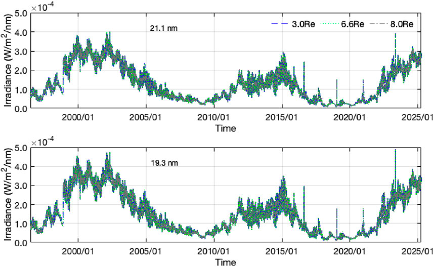
Figure 1. SSI time series at $21.1\mathrm{n}\mathrm{m}$ (top) and $19.3\mathrm{n}\mathrm{m}$ (bottom) from the CODET ${\mathrm{R}}_{\mathrm{e}}$ model at $3.0{\mathrm{R}}_{\mathrm{e}}$ (blue), $6.6{\mathrm{R}}_{\mathrm{e}}$ (green), and $8.0{\mathrm{R}}_{\mathrm{e}}$ (gray) from 1 July 1996 to 29 March 2025.

3.1 Impact of SSI from the CODET model on Earth’s upper atmosphere

The Sun–Earth interaction contributes to the atmosphere’s loss, and the Earth’s exosphere can provide important information regarding the loss mechanism. The composition of the Earth’s exosphere is dominated mainly by hydrogen, helium, and oxygen. These neutrals are lost to the interplanetary space by solar EUV photoionization and charge exchange with plasmas from the magnetosphere and the interplanetary medium (Connor et al., 2023). Solar variability, especially some events such as coronal mass ejections (CMEs), flares, or solar winds, can affect the Earth’s atmosphere; for example, geomagnetic storms can directly affect the dynamics of the exosphere (Cucho-Padin and Waldrop, 2019; Qin et al., 2017). Additionally, changes in solar activity are related to some processes such as heating efficiency, radiative cooling, thermal conduction, and dynamics in planetary exospheres (Forbes et al., 2008). The interaction of atomic hydrogen Lyman-$\alpha$ with the exosphere and plasmasphere, especially during geomagnetic storm events, is important to understand the space weather effects on Earth’s upper atmosphere (Bhattacharyya et al., 2025). In this section, the relationship between enhancements in SSI at EUV wavelengths and geomagnetic storms is explored using time series from the CODET model version 1.0 at $1\mathrm{A}\mathrm{U}$ because of the slight differences between the CODET model version 1.0 and the CODET ${\mathrm{R}}_{\mathrm{e}}$ (Figure 1). The Dst index was selected because it provides insights into how the distribution of exospheric density changes during geomagnetic storms. Previous studies have shown that there are few geomagnetic storms analyzed using the Dst index to compare the enhancements of emissions in the exosphere at distances of $3.0-8.0{\mathrm{R}}_{\mathrm{e}}$ (Cucho-Padin and Waldrop, 2019; Bailey and Gruntman, 2013). To analyze the impact of SSI on Earth’s atmosphere–exosphere along solar cycles, daily values of the geomagnetic Dst and Ap indices were used. Daily Dst values are available from the World Data Center for Geomagnetism, Kyoto¹, and the Ap index is provided by the GeoForschungsZentrum (GFZ) Potsdam² from 01 July 1996 to 29 March 2025, covering the last solar cycles.

Figure 2 shows SSI from the CODET model version 1.0 and SSI from the solar chromosphere using the Lyman-$\alpha$³ time series. The Lyman-$\alpha$ time series was selected for its significance in the exosphere and its relationship with exospheric density (Zoennchen et al., 2015). Furthermore, the exosphere is mainly populated with hydrogen, which resonantly scatters solar Lyman-$\alpha$ photons, producing the geocorona or the global glow that surrounds the Earth (Zoennchen et al., 2024).

Figure 2

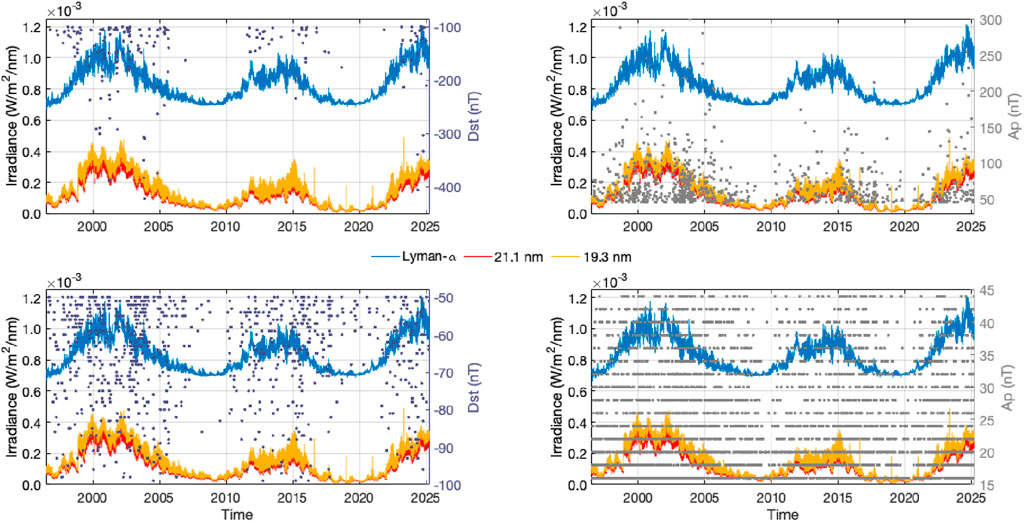
Figure 2. SSI time series at $21.1\mathrm{n}\mathrm{m}$ (red) and $19.3\mathrm{n}\mathrm{m}$ (orange) from the CODET model version 1.0 at $1\mathrm{A}\mathrm{U}$ and the Lyman-$\alpha$ at $121.427\mathrm{n}\mathrm{m}$ (blue). Daily Dst and Ap indices for strong (top) and moderate (bottom) geomagnetic storms from 01 July 1996 to 29 March 2025.

To analyze the impact of geomagnetic storms through Dst and Ap indices, two different geomagnetic regimes were defined for strong Dst $\le -100\mathrm{n}\mathrm{T}$ (Rodríguez Gómez et al., 2020) and moderate $-100\mathrm{n}\mathrm{T}>$ Dst $\le -50\mathrm{n}\mathrm{T}$ geomagnetic storms. It is important to highlight that more negative Dst values indicate larger geomagnetic activity and stronger geomagnetic storms. In addition, the Ap index intervals were defined for strong Ap $>45\mathrm{n}\mathrm{T}$ and moderate $15\mathrm{n}\mathrm{T}<$ Ap $\le 45\mathrm{n}\mathrm{T}$ geomagnetic storms (Takalo, 2021). These values were overplotted on the SSI time series during solar cycles 23 and 24 and the ascending phase of solar cycle 25. In the Earth’s case, strong geomagnetic storms are correlated with high values of SSI in EUV from coronal and chromospheric emissions at $1\mathrm{A}\mathrm{U}$ (the top panel of Figure 2) and occur preferentially during the maximum of each solar cycle. Moderate geomagnetic storms occurred during the increasing, maximum, and decreasing phases of the solar cycles (the bottom panel of Figure 2). However, their relationship is not simple, especially during moderate geomagnetic storms. Most of the strong geomagnetic storms, as indicated by the Dst and Ap indices, appear to be related to SSI values higher than their mean value. This is in agreement with the maximum of solar activity (Figure 2).

Additionally, the chromospheric emission in Lyman-$\alpha$ at $121.427\mathrm{n}\mathrm{m}$ was plotted to compare it with SSI from the CODET model. The Lyman-$\alpha$ dataset is derived from the linear correlation of Lyman-$\alpha$ line profiles observed by SOHO/SUMER (Lemaire et al., 2015), with the Lyman-$\alpha$ composite (Woods et al., 2000) producing a daily high-resolution irradiance profile (Kretzschmar et al., 2018). This chromospheric emission was included in this analysis due to its importance in the study of planetary atmospheres. In addition, it provides additional information from the solar atmosphere that it not provided by the CODET model, which focuses on emissions in the solar coronal wavelengths. SSI from the CODET model version 1.0 is compared with chromospheric emissions in Lyman-$\alpha$ at $121.427nm$ using the mean intensity ratio $\frac{\mathrm{L}\mathrm{y}\mathrm{m}\mathrm{a}\mathrm{n}-\alpha }{{\mathrm{C}\mathrm{O}\mathrm{D}\mathrm{E}\mathrm{T}}_{21.1nm}}\sim 6.58$ and $\frac{\mathrm{L}\mathrm{y}\mathrm{m}\mathrm{a}\mathrm{n}-\alpha }{{\mathrm{C}\mathrm{O}\mathrm{D}\mathrm{E}\mathrm{T}}_{19.3nm}}\sim 5.54$. It shows some differences because SSI comes from a different height in the solar atmosphere. These values are helpful for inter-comparison between SSI from different heights of the solar atmosphere. Figure 3 shows scatter plots comparing modeled SSI from the CODET model at $21.1\mathrm{n}\mathrm{m}$ and $19.3\mathrm{n}\mathrm{m}$ with SSI in Lyman-$\alpha$. Both wavelengths show a linear relationship with SSI in Lyman-α with a correlation coefficient of $\mathrm{R}=0.854$. It reflects how the modeled SSI from the CODET model and Lyman-$\alpha$ irradiance provide a good description of solar variability ranging from days to solar cycles.

Figure 3

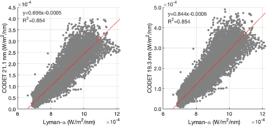
Figure 3. Scatter plots of SSI from the CODET model at 21.1 nm (left) and 19.3 nm (right) versus SSI in Lyman-α from 1 July 1996 to 29 March 2025.

It is well-known that solar irradiance affects the exosphere. However, the duration and extent of the changes in exospheric density due to variations in solar irradiance and during geomagnetic storms throughout the solar cycles remain unclear. Recently, Zoennchen and Cucho-Padin (2025) showed that density distributions during weak geomagnetic disturbances at $3.0{\mathrm{R}}_{\mathrm{e}}$–$6.0{\mathrm{R}}_{\mathrm{e}}$ are highly variable. This highlights that the relationships involved are complex, especially during both strong and weak geomagnetic storms.

4 SSI modeled at Mars $\sim 1.5\mathrm{A}\mathrm{U}$

The SSI modeled at Mars can be obtained using an adapted version of the CODET model version 1.0 and 1.1 at $28.4\mathrm{n}\mathrm{m}$ and $21.1\mathrm{n}\mathrm{m}$, respectively (Rodríguez Gómez, 2025; Rodríguez Gómez et al., 2018; Rodríguez-Gómez, 2017; Rodríguez Gómez, 2025). The modeled SSI was integrated at an average distance of $\sim 1.5\mathrm{A}\mathrm{U}$ between the Sun and Mars. MAVEN/EUVM (Eparvier et al., 2015) level-3 daily average data⁴ were used to compare the model outputs. Figure 4 shows the modeled SSI at Mars’ distance from the ${\text{CODET}}_{\text{Mars}}$ model at $28.4\mathrm{n}\mathrm{m}$ and $21.1\mathrm{n}\mathrm{m}$. The mean intensity ratio between the ${\text{CODET}}_{\text{Mars}}$ model and MAVEN data was obtained in order to guide the search for empirical factors. The mean intensity ratio for the period from 19 October 2014 to 20 April 2024 corresponds to $\frac{\mathrm{M}\mathrm{A}\mathrm{V}\mathrm{E}\mathrm{N}28.5nm}{{\mathrm{C}\mathrm{O}\mathrm{D}\mathrm{E}\mathrm{T}}_{\text{Mars}}28.4}\sim 1.31$ and $\frac{\mathrm{M}\mathrm{A}\mathrm{V}\mathrm{E}\mathrm{N}21.5nm}{{\mathrm{C}\mathrm{O}\mathrm{D}\mathrm{E}\mathrm{T}}_{\text{Mars}}21.1}\sim 3.15$. These values were used as a starting point to align SSI from the CODET model versions 1.0 and 1.1 with the MAVEN/EUVM time series at each wavelength to find the best match. In parallel, scatter plots (Figure 5) and the correlation coefficient (R) were analyzed. If the correlation coefficient was $\mathrm{R}\ge 0.80$ and the mean absolute percentage error was $ϵ<50\%$, the empirical factor was selected. Thus, these modeled time series were corrected by an empirical factor of 1.8 at $28.4\mathrm{n}\mathrm{m}$ and 4.5 at $21.1\mathrm{n}\mathrm{m}$ (Figure 4). These values differ at each wavelength because of differences in the model CODET versions 1.0 and 1.1. Each model used different observational data, namely, TIMED/SEE (CODET v 1.0) and EVE/SDO (CODET v 1.1), to constrain the model outputs. As a result, the baseline for both model versions is different (more details in Rodríguez Gómez (2025)). Additionally, these empirical factors are related to solar phase shifting, distance scaling, the different orbital radii, revolution speeds of the planet, and solar rotation. As a result, there are spatiotemporal differences in the SSI received on the planet (Xu and Qin, 2024; Thiemann et al., 2017).

Figure 4

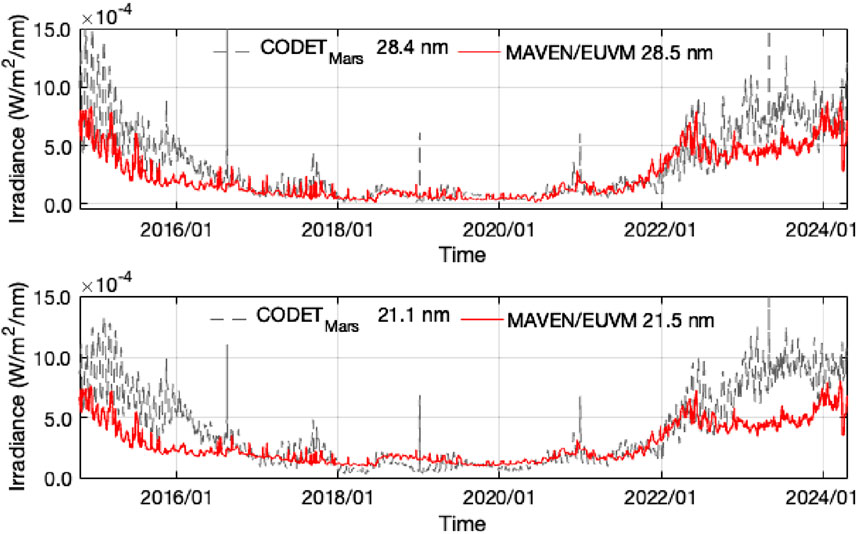
Figure 4. SSI time series at $28.4\mathrm{n}\mathrm{m}$ and $21.1\mathrm{n}\mathrm{m}$ from the ${\text{CODET}}_{\text{Mars}}$ model (gray dotted line) and the MAVEN/EUVM time series at $28.5\mathrm{n}\mathrm{m}$ and $21.5\mathrm{n}\mathrm{m}$ (red line) from 19 October 2014 to 20 April 2024.

The best model performance was obtained at both wavelengths from 6 July 2016 to 15 October 2022 (during the minimum between the solar cycles 24 and 25). In general, SSI from ${\text{CODET}}_{\text{Mars}}$ shows good agreement with the observational data from MAVEN/EUVM, with a mean absolute percentage error $(ϵ)$ of $42.21\%$ at $28.4\mathrm{n}\mathrm{m}$ and $43.92\%$ at $21.1\mathrm{n}\mathrm{m}$. The correlation coefficient (R) analysis shows a linear relationship between modeled irradiance and MAVEN/EUVM data at both wavelengths ($\mathrm{R}=0.851$ at $28.4\mathrm{n}\mathrm{m}$ and $\mathrm{R}=0.831$ at $21.1\mathrm{n}\mathrm{m}$) (Figure 5), where the model showed a good performance. These time series can help study the response of Mars’ exosphere over long-term scales, ranging from days to years.

Figure 5

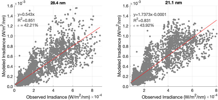
Figure 5. Solar spectral irradiance observed by MAVEN/EUVM and modeled using the ${\text{CODET}}_{\text{Mars}}$model at $28.4\mathrm{n}\mathrm{m}$(left) and at $21.1\mathrm{n}\mathrm{m}$(right) wavelengths from 19 October 2014 to 20 April 2024 scatter plots.

5 Summary and discussion

Due to the CODET model’s versatility, it is possible to obtain SSI time series at different geocentric and heliocentric distances, providing a remarkable opportunity to study planetary atmospheres even when no observational data are available. The results of this study can be summarized as follows.

$•$ SSI from the CODET model version 1.0 is presented as an alternative to F10.7 and as a valuable tool for studying planetary exospheres. It provides long time series of SSI in EUV, especially the emission originating from the solar corona, where the solar photospheric magnetic field is available. It is important to highlight that the CODET model only provides solar emission from coronal heights. Thus, it is not possible to obtain SSI from chromospheric wavelengths with the current model versions, namely, Lyman-$\alpha$ and He II $304\mathring{A}$. However, it is possible to observe how SSI from chromospheric and coronal heights follows the variation in the solar cycle, providing a comprehensive description of SSI variability over long timescales, ranging from days to solar cycles. The variability of solar irradiance significantly affects exospheric density and thermosphere heating during the solar cycle. Thus, the solar irradiance time series from the CODET model provide an important tool for understanding thermosphere–ionosphere dynamics across multiple timescales, ranging from days to solar cycles.

$•$ SSI from the CODET model version 1.0 at $1\mathrm{A}\mathrm{U}$ and the model at different geocentric distances (CODET ${\mathrm{R}}_{\mathrm{e}}$) at $3.0{\mathrm{R}}_{\mathrm{e}}$, $6.6{\mathrm{R}}_{\mathrm{e}}$, and $8.0{\mathrm{R}}_{\mathrm{e}}$ from 01 July 1996 to 29 March 2025 shows that the expected behavior due to the SSI decreases with increasing distance from the Sun following an inverse square law. However, SSI values from the CODET ${\mathrm{R}}_{\mathrm{e}}$ model and the CODET model v 1.0 at $1\mathrm{A}\mathrm{U}$ are comparable. Thus, the SSI time series from CODET ${\mathrm{R}}_{\mathrm{e}}$ can be a valuable tool to study Earth’s exosphere dynamics in detail when exospheric observations are available.

$•$ The impact of solar activity is reflected in the planetary atmospheres, for example, through geomagnetic storms and other effects. In the Earth’s case, strong geomagnetic storms are correlated with high values of SSI in EUV at $1\mathrm{A}\mathrm{U}$, preferentially during the maximum of each solar cycle. Meanwhile, moderate geomagnetic storms occur along the solar cycle, especially during the increasing, maximum, and decreasing phases of the solar cycle. However, the relationship between geomagnetic storms and exosphere variability is not completely clear; Earth’s exosphere has a complex response during geomagnetic storms. Thus, the CODET ${\mathrm{R}}_{\mathrm{e}}$ model at different geocentric distances can be used to characterize exosphere variability, such as enhancements of geocoronal emissions during and after geomagnetic storms over long timescales. It also captures more events from the last solar cycles, providing insights into the exosphere’s response and dynamics.

$•$ The SSI time series obtained from the ${\text{CODET}}_{\text{Mars}}$ model provides a valuable opportunity to study Mars’ atmosphere–exosphere. It can be an important tool for studying Mars’ exosphere, particularly the temperature changes related to EUV variability $(\sim 27\mathrm{d}\mathrm{a}\mathrm{y}\mathrm{s})$. The current version of the ${\text{CODET}}_{\text{Mars}}$ model shows good performance during the minimum between solar cycles 24 and 25 and the ascending phase of solar cycle 25. However, SSI from the CODET model can be improved in future versions by incorporating the solar magnetic field contributions from the far side and obtaining SSI at specific locations on Mars. The Sun’s far-side magnetic flux can provide an accurate magnetic field evolution and, in turn, improve SSI modeling. The Sun’s far-side magnetic field cannot be directly observed; however, helioseismic imaging techniques (Lindsey and Braun, 2000) and, more recently, machine learning models (Chen et al., 2022) can provide accurate global solar magnetic field maps, including those of the near and far sides.

Data availability statement

The datasets presented in this study can be found in online repositories. The names of the repository/repositories and accession number(s) can be found at: https://github.com/Rodriguez-Gomez/CODET_geocentric.git https://github.com/Rodriguez-Gomez/CODET_Mars.git.

Author contributions

JR-G: Funding acquisition, Validation, Software, Methodology, Formal Analysis, Writing – original draft, Conceptualization, Investigation.

Funding

The author(s) declare that financial support was received for the research and/or publication of this article. This work was supported by NASA Living With a Star (LWS) Program, Focused Science Topic: “Beyond F10.7: Quantifying Solar EUV Flux and its Impact on the Ionosphere–Thermosphere–Mesosphere System,” No. 80NSSC23K0900.

Conflict of interest

The author declares that this research was conducted in the absence of any commercial or financial relationships that could be construed as a potential conflict of interest.

Generative AI statement

The author(s) declare that no Generative AI was used in the creation of this manuscript.

Any alternative text (alt text) provided alongside figures in this article has been generated by Frontiers with the support of artificial intelligence and reasonable efforts have been made to ensure accuracy, including review by the authors wherever possible. If you identify any issues, please contact us.

Publisher’s note

All claims expressed in this article are solely those of the authors and do not necessarily represent those of their affiliated organizations, or those of the publisher, the editors and the reviewers. Any product that may be evaluated in this article, or claim that may be made by its manufacturer, is not guaranteed or endorsed by the publisher.

Footnotes

¹https://wdc.kugi.kyoto-u.ac.jp/dstae/index.html

²https://www.gfz.de/en/section/geomagnetism/data-products-services/geomagnetic-kp-index

³https://lasp.colorado.edu/lisird/data/lyman_alpha_model_ssi

⁴https://lasp.colorado.edu/lisird/data/mvn_euv_l3_daily

References

Bailey, J., and Gruntman, M. (2013). Observations of exosphere variations during geomagnetic storms. grl 40, 1907–1911. doi:10.1002/grl.50443

CrossRef Full Text | Google Scholar

Bhattacharyya, D., Thiemann, E. M. B., Machol, J., Cucho-Padin, G., Chatterjee, S., Harris, W., et al. (2025). The hydrogen lyman α line shape in the exospheres of terrestrial objects in the solar system. Front. Astronomy Space Sci. 12. doi:10.3389/fspas.2025.1589784

CrossRef Full Text | Google Scholar

Carlesso, F., Rodríguez Gómez, J. M., Barbosa, A. R., Antunes Vieira, L. E., and Dal Lago, A. (2022). Solar irradiance variability monitor for the galileo solar space telescope mission: concept and challenges. Front. Phys., 10–2022. doi:10.3389/fphy.2022.869738

CrossRef Full Text | Google Scholar

Chamberlin, P. C., Hock, R. A., Crotser, D. A., Eparvier, F. G., Furst, M., Triplett, M. A., et al. (2007). “EUV variability experiment (EVE); multiple EUV grating spectrographs (MEGS), radiometric calibrations and results,” in Solar physics and space weather instrumentation II. Editors S. Fineschi, and R. A. Viereck (Society of Photo-Optical Instrumentation Engineers (SPIE) Conference Series), 66890N, 66890N. doi:10.1117/12.734116

CrossRef Full Text | Google Scholar

Chamberlin, P. C., Woods, T. N., and Eparvier, F. G. (2008). Flare irradiance spectral model (FISM): flare component algorithms and results. Space weather. 6, S05001. doi:10.1029/2007SW000372

CrossRef Full Text | Google Scholar

Chen, R., Zhao, J., Hess Webber, S., Liu, Y., Hoeksema, J. T., and DeRosa, M. L. (2022). Inferring maps of the sun’s far-side unsigned magnetic flux from far-side helioseismic images using machine learning techniques. apj 941, 197. doi:10.3847/1538-4357/aca333

CrossRef Full Text | Google Scholar

Connor, H., Jung, J., Claudepierre, S., Mierkiewicz, E., Zhang, Y., Pham, K., et al. (2023). The Earth’s exosphere and its response to space weather. Bull. AAS 55. doi:10.3847/25c2cfeb.523ff599

CrossRef Full Text | Google Scholar

Cucho-Padin, G., and Waldrop, L. (2019). Time-dependent response of the terrestrial exosphere to a geomagnetic storm. grl 46 (11), 661–670. doi:10.1029/2019GL084327

CrossRef Full Text | Google Scholar

Cucho-Padin, G., Bhattacharyya, D., Sibeck, D. G., Connor, H., Youngblood, A., and Ardila, D. (2023). EXOSpy: a python package to investigate the terrestrial exosphere and its FUV emission. Front. Astronomy Space Sci. 10, 1082150. doi:10.3389/fspas.2023.1082150

CrossRef Full Text | Google Scholar

Delgado-Bonal, A., Zorzano, M.-P., and Martín-Torres, F. J. (2016). Martian top of the atmosphere 10–420nm spectral irradiance database and forecast for solar cycle 24. Sol. Energy 134, 228–235. doi:10.1016/j.solener.2016.05.004

CrossRef Full Text | Google Scholar

Eparvier, F. G., Chamberlin, P. C., Woods, T. N., and Thiemann, E. M. B. (2015). The solar extreme ultraviolet monitor for MAVEN. ssr 195, 293–301. doi:10.1007/s11214-015-0195-2

CrossRef Full Text | Google Scholar

Forbes, J. M., Bruinsma, S., and Lemoine, F. G. (2006). Solar rotation effects on the thermospheres of Mars and earth. Science 312, 1366–1368. doi:10.1126/science.1126389

PubMed Abstract | CrossRef Full Text | Google Scholar

Forbes, J. M., Lemoine, F. G., Bruinsma, S. L., Smith, M. D., and Zhang, X. (2008). Solar flux variability of mars’ exosphere densities and temperatures. grl 35, L01201. doi:10.1029/2007GL031904

CrossRef Full Text | Google Scholar

Hock, R. A., and Eparvier, F. G. (2008). Cross-calibration of TIMED SEE and SOHO EIT irradiances. solphys 250, 207–219. doi:10.1007/s11207-008-9203-y

CrossRef Full Text | Google Scholar

Hock, R. A., Chamberlin, P. C., Woods, T. N., Crotser, D., Eparvier, F. G., Woodraska, D. L., et al. (2012). Extreme ultraviolet variability experiment (EVE) multiple EUV grating spectrographs (MEGS): Radiometric calibrations and results. solphys 275, 145–178. doi:10.1007/s11207-010-9520-9

CrossRef Full Text | Google Scholar

Kretzschmar, M., Snow, M., and Curdt, W. (2018). An empirical model of the variation of the solar Lyman-α spectral irradiance. grl 45, 2138–2144. doi:10.1002/2017GL076318

CrossRef Full Text | Google Scholar

Krishnamurthy, V., and Cowan, N. B. (2024). Helium in exoplanet exospheres: orbital and stellar influences. aj 168, 30. doi:10.3847/1538-3881/ad5441

CrossRef Full Text | Google Scholar

Lammer, H., Kulikov, Y. N., and Lichtenegger, H. I. M. (2006). Thermospheric X-Ray and euv heating by the young sun on early Venus and Mars. ssr 122, 189–196. doi:10.1007/s11214-006-7018-4

CrossRef Full Text | Google Scholar

Lemaire, P., Vial, J. C., Curdt, W., Schühle, U., and Wilhelm, K. (2015). Hydrogen Ly-αand Ly-βfull sun line profiles observed with SUMER/SOHO (1996–2009). Hydrogen Ly-α Ly-β full Sun line profiles observed SUMER/SOHO (1996-2009). aap 581, A26. doi:10.1051/0004-6361/201526059

CrossRef Full Text | Google Scholar

Lindsey, C., and Braun, D. C. (2000). Seismic images of the far side of the sun. Science 287, 1799–1801. doi:10.1126/science.287.5459.1799

PubMed Abstract | CrossRef Full Text | Google Scholar

Linsky, J. (2014). The radiation environment of exoplanet atmospheres. Challenges 5, 351–373. doi:10.3390/challe5020351

CrossRef Full Text | Google Scholar

Qin, J., Waldrop, L., and Makela, J. J. (2017). Redistribution of H atoms in the upper atmosphere during geomagnetic storms. J. Geophys. Res. Space Phys. 122 (10), 686–693. doi:10.1002/2017JA024489

CrossRef Full Text | Google Scholar

Rodríguez Gómez, J. M. (2025). Modeling solar spectral irradiance (SSI) from iron lines using the CODET model version 1.1. apj 985, 10. doi:10.3847/1538-4357/adcec6

CrossRef Full Text | Google Scholar

Rodríguez Gómez, J. M., Vieira, L., Dal Lago, A., and Palacios, J. (2018). Coronal electron density temperature and solar spectral irradiance during solar cycles 23 and 24. apj 852, 137. doi:10.3847/1538-4357/aa9f1c

CrossRef Full Text | Google Scholar

Rodríguez Gómez, J. M., Palacios, J., Vieira, L. E. A., and Dal Lago, A. (2019). The plasma β evolution through the solar Corona during solar cycles 23 and 24. apj 884, 88. doi:10.3847/1538-4357/ab40af

CrossRef Full Text | Google Scholar

Rodríguez Gómez, J. M., Podladchikova, T., Veronig, A., Ruzmaikin, A., Feynman, J., and Petrukovich, A. (2020). Clustering of fast coronal mass ejections during solar cycles 23 and 24 and the implications for CME-CME interactions. apj 899, 47. doi:10.3847/1538-4357/ab9e72

CrossRef Full Text | Google Scholar

Rodríguez-Gómez (2017). Modeling density and temperature profiles in the solar corona based on solar surface magnetic field observations during the solar cycle 23 and 24. Ph.D. thesis, Instituto Nacional de Pesquisas Espaciais INPE, Brasil. Available online at: http://urlib.net/8JMKD3MGP3W34P/3NCJQLB

Google Scholar

Scherrer, P. H., Bogart, R. S., Bush, R. I., Hoeksema, J. T., Kosovichev, A. G., Schou, J., et al. (1995). The solar oscillations investigation - Michelson doppler imager. solphys 162, 129–188. doi:10.1007/BF00733429

CrossRef Full Text | Google Scholar

Scherrer, P. H., Schou, J., Bush, R. I., Kosovichev, A. G., Bogart, R. S., Hoeksema, J. T., et al. (2012). The helioseismic and magnetic imager (HMI) investigation for the solar dynamics Observatory (SDO). solphys 275, 207–227. doi:10.1007/s11207-011-9834-2

CrossRef Full Text | Google Scholar

Schrijver, C. J. (2001). Simulations of the photospheric magnetic activity and outer atmospheric radiative losses of cool stars based on characteristics of the solar magnetic field. apj 547, 475–490. doi:10.1086/318333

CrossRef Full Text | Google Scholar

Schrijver, C. J., and De Rosa, M. L. (2003). Photospheric and heliospheric magnetic fields. solphys 212, 165–200. doi:10.1023/A:1022908504100

CrossRef Full Text | Google Scholar

Takalo, J. (2021). Comparison of geomagnetic indices during Even and odd Solar cycles SC17 - SC24: signatures of gnevyshev gap in geomagnetic activity. solphys 296, 19. doi:10.1007/s11207-021-01765-w

CrossRef Full Text | Google Scholar

Thiemann, E. M. B., Chamberlin, P. C., Eparvier, F. G., Templeman, B., Woods, T. N., Bougher, S. W., et al. (2017). The MAVEN EUVM model of solar spectral irradiance variability at Mars: algorithms and results. J. Geophys. Res. Space Phys. 122, 2748–2767. doi:10.1002/2016JA023512

CrossRef Full Text | Google Scholar

Woods, T. N., Tobiska, W. K., Rottman, G. J., and Worden, J. R. (2000). Improved solar lyman α irradiance modeling from 1947 through 1999 based on UARS observations. jgr 105, 27195–27215. doi:10.1029/2000JA000051

CrossRef Full Text | Google Scholar

Woods, T. N., Eparvier, F. G., Bailey, S. M., Chamberlin, P. C., Lean, J., Rottman, G. J., et al. (2005). Solar EUV experiment (SEE): mission overview and first results. J. Geophys. Res. Space Phys. 110, A01312. doi:10.1029/2004JA010765

CrossRef Full Text | Google Scholar

Woods, T. N., Eparvier, F. G., Hock, R., Jones, A. R., Woodraska, D., Judge, D., et al. (2012). Extreme ultraviolet variability experiment (EVE) on the solar dynamics observatory (SDO): overview of science objectives, instrument design, data products, and model developments. solphys 275, 115–143. doi:10.1007/s11207-009-9487-6

CrossRef Full Text | Google Scholar

Xu, Z., and Qin, J. (2024). A comparative analysis of the solar ultraviolet spectral irradiance measured from Earth and Mars: toward a general empirical model for the study of planetary aeronomy. apjs 271, 11. doi:10.3847/1538-4365/ad17c2

CrossRef Full Text | Google Scholar

Zoennchen, J. H., and Cucho-Padin, G. (2025). The response of exospheric neutral hydrogen to weak geomagnetic disturbances between June 12 and 29, 2008. Front. Astronomy Space Sci. 12, 1536249. doi:10.3389/fspas.2025.1536249

CrossRef Full Text | Google Scholar

Zoennchen, J. H., Nass, U., and Fahr, H. J. (2015). Terrestrial exospheric hydrogen density distributions under solar minimum and solar maximum conditions observed by the twins stereo mission. Ann. Geophys. 33, 413–426. doi:10.5194/angeo-33-413-2015

CrossRef Full Text | Google Scholar

Zoennchen, J. H., Cucho-Padin, G., Waldrop, L., and Fahr, H. J. (2024). Comparison of terrestrial exospheric hydrogen 3d distributions at solar minimum and maximum using twins lyman-α observations. Front. Astronomy Space Sci. 11, 1409744. doi:10.3389/fspas.2024.1409744

CrossRef Full Text | Google Scholar