 Kun Zhang
 Yanshi Huang
 Fengsi Wei1,2
 Pingbing Zuo
 Hao Yang
 Jinlong Ji
- 1Shenzhen Key Laboratory of Numerical Prediction for Space Storm, School of Aerospace, Harbin Institute of Technology, Shenzhen, China
- 2Key Laboratory of Solar Activity and Space Weather, National Space Science Center, Chinese Academy of Sciences, Beijing, China
- 3China Mobile Construction Co., Ltd., Beijing, Hebei, China
Temporal variation and spatial distribution of the thermospheric density can change significantly during geomagnetic storms. These variations in thermospheric density enhance atmospheric drag, posing risks to Low-Earth-Orbit (LEO) spacecraft. Therefore, studying the characteristics of intense storm-time thermospheric density perturbations and orbit decay is crucial for practical applications. In this study, neutral density was simulated for the strongest magnetic storm events of solar cycles 24, 23, and 22, corresponding to minimum Dst indices of −234 nT (2015 St. Patrick’s Day storm), −442 nT (20 November 2003 storm), and −598 nT (1989 Quebec blackout storm). Four representative thermospheric models (DTM-2020, JB 2008, NRLMSIS 2.0, and TIEGCM 2.0) were employed to evaluate their performance during extreme geomagnetic storms by comparing simulated densities with satellite observations from Swarm, CHAMP, and GRACE during the November 2003 and March 2015 storm events. The results indicate that the errors of all models exhibit larger errors in the main and recovery phases, with a bias toward underestimation of density during the main phase. It is important to note that no thermospheric model is perfect and each model has its own limitations, especially dealing with extreme space weather events. Although JB2008 performs relatively well, it does not maintain the best performance across all phases, and its predictions still deviate from observations by at least 20%. Therefore, combining multiple model outputs is recommended for extreme cases. Furthermore, these thermospheric models were coupled with the High-Precision Orbit Propagator (HPOP) to examine the orbital decay of the China Space Station (CSS, ∼380–400 km altitude) during these events. The effects of drag on CSS during the strongest magnetic storm events in the 24th, 23rd and 22nd solar cycles were simulated. The orbital decay is about 233%, 300% and 266% higher than that in the quiet period, respectively. The reults of this study might serve as a reference for spacecraft for possible upcoming extreme magnetic storm events.
1 Introduction
The space environment has a significant impact on spacecraft launches and operations. During geomagnetic storms, thermospheric neutral density can fluctuate by several orders of magnitude (Qian and Solomon, 2012), causing instabilities in the orbits and attitudes of spacecraft and space debris. This phenomenon increases the risk of spacecraft collisions and poses a serious threat to the safety of spacecraft operations in orbit (Richmond et al., 1992; Thirsk et al., 2009; Berger et al., 2023). Historically, in 1979, the Skylab space station failed to maintain orbital stability and re-entered Earth’s atmosphere 2 years earlier than expected due to a severe underestimation of the space environmental effects (Sivolella, 2022). The CSS, completed in November 2022, serves as a crucial platform for long-term human space habitation and future space exploration (Gu, 2022). It is designed for a lifespan of up to 15 years, with an orbital altitude of 380–400 km, lower than that of the International Space Station (ISS), resulting in more significant drag effects (DeLucas, 1996). Therefore, analyzing the orbital decay of the CSS during geomagnetic storms is essential for safeguarding its operational safety (Briden et al., 2022; Lechtenberg et al., 2013; Dang et al., 2022).
The thermospheric environment is a major factor influencing the prediction of spacecraft drag. In aerospace engineering, thermospheric models provide parameters such as density, temperature, and composition to predict aerodynamic drag on satellites and space debris (Oliveira and Zesta, 2019; Zhang et al., 2022). Thermospheric models developed in recent decades are broadly classified into two categories: first-principle physical models and empirical models (Bruinsma et al., 2021). Physical models solve the fluid equations numerically to describe the coupled ionosphere-thermosphere (IT) system (Ren and Lei, 2023). Empirical models, also known as statistical models, represent the statistically averaged behavior of the thermosphere using parameterized mathematical formulations. Several studies have investigated the application of thermospheric models to satellite orbits. Ya-Ying and Zhao (1995) analyzed the effects of various thermospheric models during periods of high and low solar activity on the orbital lifetime and propellant fuel consumption of a space station. Liu, (2015) adopted the Naval Research Laboratory Mass Spectrometer Incoherent Scatter Model (NRLMSIS) to reveal the correlation between the drag coefficient of Tiangong-1 and space environment parameters using wavelet transform analysis.
In the 1980s, Gaposchkin, (1994) conducted a comparative analysis of various thermospheric models and concluded that no single model could satisfy all satellite missions. To date, this issue remains unresolved, despite the development of additional models (He et al., 2018). Li et al. (2014) explored the differences between modeled and observed values of thermospheric density during various geomagnetic disturbances. Their findings indicate that thermospheric models perform poorly during geomagnetic storms and require further improvement. Emmert (2015) examined the construction principles of various thermospheric models and analyzed their advantages and characteristics. Therefore, employing multiple models for density estimation may be an effective approach when addressing strong space weather events (Elvidge et al., 2016). In this study, we employ one first-principle physical model, the Thermosphere-Ionosphere-Electrodynamics General Circulation Model (TIEGCM 2.0; Roble et al., 1988; Richmond et al., 1992), together with one empirical model, the Naval Research Laboratory Mass Spectrometer and Incoherent Scatter Model (NRLMSIS; Picone et al., 2002), and two semi-empirical models, the Drag Temperature Model (DTM-2020; Bruinsma and Boniface, 2021) and the Jacchia–Bowman Model (JB-2008; Bowman et al., 2007), to estimate thermospheric density.
During intense space weather events, such as severe geomagnetic storms, substantial electromagnetic energy flows into the ionosphere-thermosphere (IT) system, causing rapid thermospheric heating and vertical expansion due to collisions between ions and neutral particles (Prölss 2011; Emmert, 2015). Accordingly, satellites passing through these regions experience increased drag forces, leading to more severe orbital degradation or altitude losses (Prieto et al., 2014; Zesta and Huang, 2016). Oliveira et al. (2020) examined four historical magnetic super storms, showing that, as expected, orbital degradation is more severe during stronger storms. Furthermore, the results clearly indicate that storm duration is significantly correlated with the impact of orbital drag effects and plays a key role in enhancing drag. During the 60 h of storm activity in November 2003, the CHAllenge Mini-satellite Payload (CHAMP) and Gravity Recovery and Climate Experiment (GRACE) satellites experienced orbital decays of approximately 160 m and 71 m, respectively (Krauss et al., 2015). These values are substantially greater than the orbital decay expected under quiet-time density conditions, being about 5.63 and 9.44 times higher, respectively (Oliveira and Zesta, 2019). Chen et al. (2014) conducted a statistical analysis to study the impact of different types of storms on satellite orbital decay. The results indicate that Corotating Interaction Region (CIR) driven storms have a slightly larger impact on total orbital decay compared to Coronal Mass Ejection (CME)-driven storms, since CIR storms significantly affect thermospheric density and satellite orbits due to their prolonged duration. Improved understanding and management of orbital drag during geomagnetic storms can enhance tracking accuracy, increase reentry prediction reliability, and prolong satellite lifetimes (Berger et al., 2020).
The three events studied in this paper are all extreme space weather events caused by coronal mass ejections (CMEs). It is widely accepted in the space weather research community that intense geomagnetic storms, particularly extreme events, are typically caused by CMEs (Balan et al., 2014; Kilpua et al., 2019). Notably, the frequency and intensity of extreme events during Solar Cycles 22 to 24 gradually declined, which may be attributed to the Gleissberg Cycle approaching its minimum phase. The Gleissberg Cycle is a long-term solar activity cycle with a period of approximately 80–100 years (Gleissberg, 1965). It is superimposed on the more familiar 11-year sunspot cycle and modulates the overall intensity of solar activity. Feynman and Ruzmaikin, (2014) noted that the minimum phase of the Gleissberg Cycle nearly coincided with Solar Cycle 24. They also observed a gradual decline in the F10.7 solar flux peak from 1980 to 2021, marking Cycle 24 as the weakest in a century. According to Adams et al. (2025), proton flux variations in the South Atlantic Anomaly region may indicate the end of the Gleissberg minimum. Currently, sunspot numbers are increasing, solar ultraviolet output is strengthening, and overall activity during Solar Cycle 25 has exceeded earlier predictions. As the Gleissberg cycle is rising again, the probability and intensity of extreme space weather events are expected to increase greatly over the next few decades, making the impact of the space environment on spacecraft more severe. Several studies suggest that LEO mega-constellations such as Starlink, OneWeb, and GuoWang (GW) will expand significantly in the coming years (Oliveira et al., 2021; Zhang et al., 2022). Therefore, it is urgent to improve the accurate estimation of neutral density variations in low Earth orbit (LEO) and enhance high-precision orbit determination for spacecraft under extreme space weather conditions. Additionally, orbit maintenance strategies must be strengthened to address the potential impacts of extreme space weather events, such as the 1859 Carrington storm (an estimated minimum Dst index of −1760 nT), on spacecraft operations (Lakhina and Tsurutani, 2017).
The CSS is a crewed space station system independently built by China, consisting of the Tianhe Core Module, the Wentian Experiment Module, and the Mengtian Experiment Module. In November 2022, the Mengtian Experiment Module successfully docked with the Tianhe Core Module, forming a basic “T” configuration with the Wentian Experiment Module, marking the completion of the in-orbit assembly of the CSS. It operates in a near-circular orbit with an inclination of 41.42°. When fully assembled, it has a total mass of approximately 180 tons and can support three astronauts for long-duration missions, with accommodation for six astronauts during crew rotations.CSS serves as a national-level space laboratory with scientific objectives including supporting frontier scientific exploration, advancing space technology research, and promoting the development and utilization of space resources for the benefit of humanity. Considering that the design lifespan of CSS is 10–15 years (approximately one solar cycle), it will inevitably experience multiple severe space weather events.
In this study, we select the most geomagnetically intense storm events in 22, 23, and 24 solar cycles to evaluate the potential impacts of extreme storm events on CSS, which are the 2015 St. Patrick’s Day storm, the 20 November 2003 storm, and the 1989 Quebec blackout storm. Although CSS was not operational during these events, the storms produced thermospheric density perturbations whose mechanisms are similar to those possible in future extreme events. Themospheric density values derived by the Jacchia-Bowman 2008 (JB 2008), NRLMSIS 2.0, the Drag Temperature Model 2020 (DTM-2020), and the Thermosphere-Ionosphere-Electrodynamics General Circulation Model 2.0 (TIEGCM 2.0) models are used as the input of the orbital propagator to estimate orbital decays. Section 2 introduces the models used in this study, while Section 3 presents the experimental settings. Results are discussed in Section 4, with the summary provided in the final section.
2 Methodology
2.1 Thermospheric density models
In this study, four thermospheric models are used to provide the global neutral density, which are DTM-2020, JB 2008, NRLMSIS 2.0 and TIEGCM 2.0. The Drag Temperature Model (DTM) is a semi-empirical model that describes the temperature, density, and composition of Earth’s atmosphere (Bruinsma and Boniface, 2021). It was originally developed to accurately predict satellite drag and orbits. The model was constructed using density data derived from acceleration measurements obtained by the CHAMP, GRACE, and Gravity field and Ocean Circulation Explorer (GOCE) satellites. DTM-2020 provides two configurations, an operational mode and a research mode. The operational mode is driven by the daily F10.7 solar flux index and the 3-h Kp geomagnetic index, while the research mode employs the daily F30 solar proxy index together with the hourly geomagnetic index ap60 for more precise results (Yamazaki et al., 2022). In this study, the research mode is adopted.
The JB2008 model applies the Jacchia diffusion equation in atmospheric dynamics to compute thermospheric temperature and density across altitudes ranging from 90 to 2500 km. It incorporates acceleration data from the CHAMP (2001–2005) and GRACE (2002–2005) satellites to improve accuracy. A key advancement is its use of extreme ultraviolet (EUV) and far ultraviolet (FUV) radiation data instead of the conventional F10.7 index, combined with geomagnetic disturbance parameters (Dst and ap indices).
The NRLMSIS series is an empirical global reference model of the thermosphere, covering Earth’s atmosphere from the surface up to 1000 km. It was released by the U.S. Naval Research Laboratory in 2000 and has been widely used in space weather operations (Picone et al., 2002). NRLMSISE 2.0 (Emmert et al., 2020), released in May 2020, is a significant reformulated upgrade of the previous version, NRLMSIS-00. This model incorporates physical constraints, including hydrostatic equilibrium in the well-mixed lower atmosphere (below ∼70 km), species-specific hydrostatic equilibrium (similar to diffusive equilibrium) above ∼200 km, and relaxation of thermospheric temperature to an asymptotic exospheric temperature. In subsequent experiments we employ the NRLMSIS 2.0 version, which takes as inputs the day of year (DOY), Universal Time (UT), altitude, latitude, longitude, local solar time, the 81-day average of F10.7, the daily F10.7 of the preceding day, and the 3-h ap index.
The Thermosphere Ionosphere Electrodynamics General Circulation Model (TIEGCM, Dickinson et al., 1981; Roble et al., 1988; Richmond et al., 1992; Qian et al., 2014) is a coupled thermosphere-ionosphere physical model developed by the National Center for Atmospheric Research (NCAR). It employs finite-difference techniques to solve the kinetic, thermodynamic, and continuity equations, considering the roles of particle deposition in the polar regions, high-latitude electric fields, and tides from the lower atmosphere. In this study, the TIEGCM 2.0 is run with a 5° × 5° spatial resolution (longitude × latitude) and 5-min temporal resolution. For the 2015 and 2003 storm events, Weimer05 model (Weimer, 2005) is used to provide the high-latitude electric potential patterns, while for the 1989 storm event, Heelis model (Heelis et al., 1982) is used as the high-latitude driver due to lack of Interplanetary Magnetic Field (IMF) data.
These four thermospheric models mentioned above are used to provide the variations of neutral density along spacecraft tracks.
2.2 Orbit propagator model
In this study, the High-Precision Orbit Propagator (HPOP) model is used to estimate the orbit of CSS. HPOP calculates the change of orbital state elements, such as position and velocity, by using acceleration in the equations of motion (Refaat et al., 2018). The numerical integration algorithm approximates the spacecraft’s motion over a single integration step using a series of force model evaluations, which account for a wide range of complex drag forces. It incorporates an Earth gravity model, solid tide and sea tide models, a solar radiation pressure model, solar and lunar gravitational field models, and a thermospheric drag model, enabling accurate simulation of the satellite’s orbital state. To determine the orbital decay rates, the mean orbital elements are computed using Eckstein-Ustinov-Kaula’s (EUK) method (Spiridonova et al., 2014). The EUK method is an analytical algorithm that combines Eckstein-Ustinov’s and Kaula’s analytical theories to convert osculating orbital elements into mean orbital elements (Eckstein and Hechler, 1970; Kaula and Street, 1967). The input parameters for the HPOP include the initial orbital elements, total propagator time, step size, drag coefficient, solar radiation coefficient, effective area of the spacecraft for solar radiation and drag, and the mass of spacecraft. The HPOP model combines various orbital perturbation terms based on these initial parameters, using the Runge-Kutta Fehlberg 7 (8) integrator, and outputs the position and velocity of a spacecraft at each time step.
3 Experimental setting
To evaluate the impact of geomagnetic storm events of different intensities on the China space station, three events are selected for analysis, and four thermospheric models (JB 2008, NRLMSIS 2.0, DTM-2020, and TIEGCM 2.0) are used to provide the neutral density to the HPOP model. The three geomagnetic storm events selected are the 2015 St. Patrick’s Day storm, the 20 November 2003 storm, and the 1989 Quebec blackout storm, with minimum Dst indices of −234 nT, −442 nT, and −598 nT, respectively, as shown in Figure 1. These geomagnetic storm events are well known for causing serious hazards to spacecraft and ground systems, making them suitable cases for assessing the orbital impacts of the space station under intense space weather conditions.
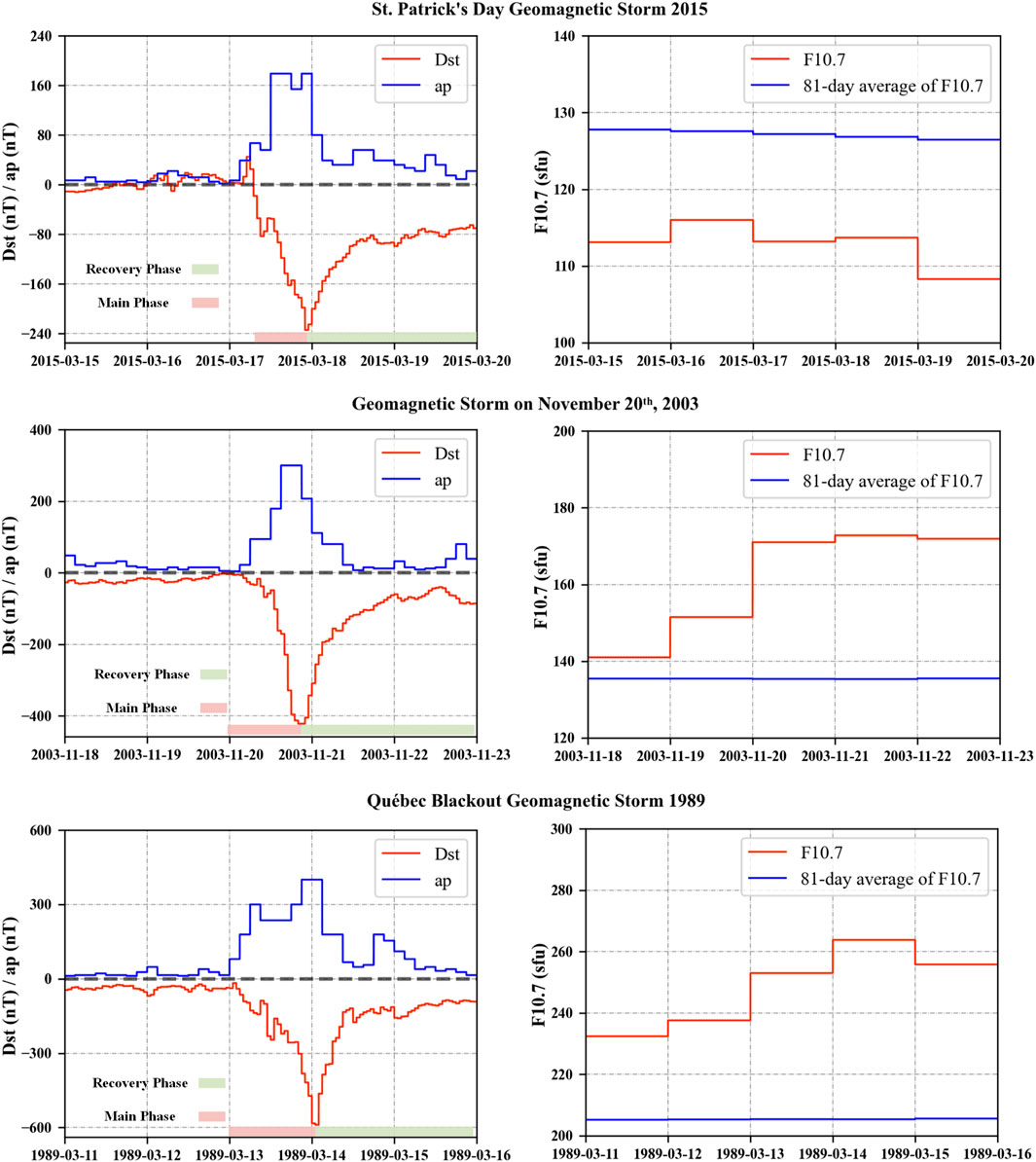
Figure 1. Temporal variations of space weather indices during the three most geomagnetically disturbed storms in solar cycles 22, 23, and 24. The left column shows geomagnetic indices (Dst and ap), while the right column presents solar activity (daily F10.7 flux and 81-day averages).
Based on the discussion above, the experimental flow is designed as shown in Figure 2, with the experimental parameters provided in Table 1. The spacecraft's thermospheric drag acceleration is given by Equation 1:
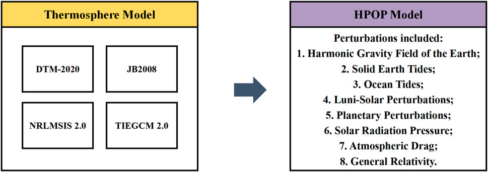
Figure 2. Experimental flow design.
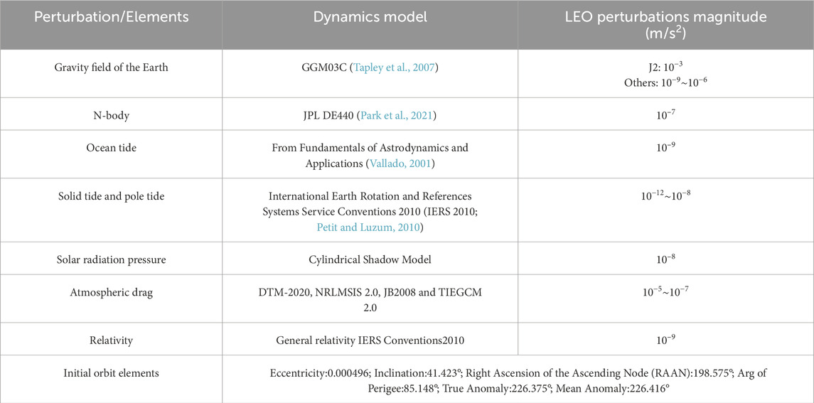
Table 1. Dynamics Models and CSS orbit elements.
When making operational decisions for CSS, the physical ballistic coefficient is determined from the interaction mechanisms between the atmosphere and the target surface. It incorporates factors such as atmospheric escape temperature, surface temperature, relative velocity, atmospheric composition, gas-surface interaction models, as well as the target’s geometry and attitude. Nevertheless, this method cannot be applied to the CSS in this study due to the lack of essential parameters.
The fitted ballistic coefficient is obtained through orbit determination inversion. With sufficient observational data, both the orbital parameters and
1. The initial state and parameters of the spacecraft are provided to the HPOP Ephemeris Computation module. The time and position are calculated using the RadauIIA integrator, and the results are forwarded to the thermosphere model.
2. The thermosphere model calculates the neutral density according to the given time, position, and space environmental parameters.
3. Next, perturbing forces (including thermospheric drag, the Earth’s harmonic gravity field, solid Earth tides, etc.) are computed using the HPOP drag module based on the given density and spacecraft state.
4. The obtained acceleration is re-entered into the Ephemeris Computation module for the next calculation. Finally, the osculating orbital elements are processed using the EUK method to derive the mean orbital elements.
4 Results
4.1 Geomagnetic storm on 17 March 2015
The intense geomagnetic storm on 17 March 2015, known as the St. Patrick’s Day storm, was the strongest storm of solar cycle 24. During this event, sudden storm commencement occurred in the early hours of March 17th when a fast-moving CME struck the Earth’s magnetic field. Initially, the CME impact produced only a minor G1-class disturbance (Kp = 5). As the Earth moved into the CME’s strongly magnetized wake, the storm intensified to a G4-class (Kp = 8) event, with a minimum Dst value of −234 nT at 22:00 UT on March 17th. Figure 3 illustrates the thermospheric density distribution at 400 km from four different models in the various phases of this geomagnetic storm. Clear enhancements of the global density during the storm main phase are noticed from the simulated results of all four models. Moreover, during the main phase, the largest density is found in the DTM-2020 simulation, whereas the smallest enhancement is found in the TIEGCM 2.0 result. Subsequently, the recovery phase began on March 18th and lasted for a few days. Analysis of the 2015 geomagnetic storm indicates that the global mean thermospheric density increased by 92.3% in DTM-2020, 109.2% in JB 2008, 76.4% in NRLMSIS 2.0, and 48.1% in TIEGCM 2.0 when comparing the main phase with quiet-time conditions.
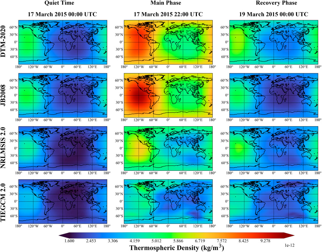
Figure 3. Global thermospheric density distributions at 400 km during the 17 March 2015 magnetic storm from different models. The rows correspond to DTM-2020 (top), JB 2008 (second), NRLMSIS 2.0 (third), and TIEGCM 2.0 (bottom), shown across the quiet, main, and recovery phases.
Figure 4 presents the comparison between thermospheric density predictions from four empirical and physical models (DTM-2020, JB 2008, NRLMSIS 2.0, and TIEGCM 2.0) and measurements from Swarm-A (upper) and GRACE-A (lower) during the geomagnetic storm event of March 15–19, 2015. The left column shows the modeled and observed densities, while the right column illustrates the corresponding percentage errors, separated into quiet, main, and recovery phases of the storm.
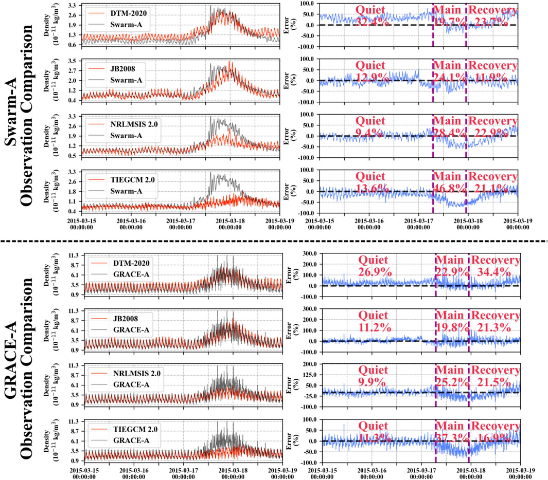
Figure 4. Comparison of the along-track density observed by satellites (Swarm-A and GRACE-A) and predicted by DTM-2020, JB 2008, NRLMSIS 2.0, and TIEGCM 2.0 models between March 15th and 19th, 2015.
For Swarm-A at an altitude of approximately 450–480 km, all models except DTM-2020 show good fitting with the observations during the quiet period, with mean errors ranging from 9.4% to 13.6%. However, during the main phase, all models underestimated the density enhancement, with TIEGCM 2.0 exhibiting the largest deviation (46.8%) and DTM-2020 the smallest (19.7%). In the recovery phase, JB2008 maintains a comparatively lower error (∼11.9%) compared to the other models, whereas NRLMSIS 2.0 and TIEGCM exhibit significant deviations.
For GRACE-A (altitude 390–420 km), a similar pattern is observed. JB2008 again provides the best overall performance, with the lowest mean errors across all storm phases (11.2%, 19.8%, and 21.3%, respectively). DTM-2020 and NRLMSIS 2.0 show moderate accuracy, with noticeable underestimations during the main phase (errors exceeding 20%). In contrast, TIEGCM 2.0 persistently underestimated the density enhancement at the onset of the storm, with an error exceeding 37% during the main phase.
Obvious density underestimation is demonstrated in the results of NRLMSIS 2.0 and TIEGCM 2.0 during the main phase of 2015 magnetic storm event. And JB2008 shows the most consistent performance for both Swarm-A and GRACE-A satellites during the whole storm, whereas TIEGCM 2.0 exhibits the largest deviations from observations. The relatively low densities simulated by TIEGCM 2.0 are likely due to the lack of high-latitude energy input during the geomagnetically disturbed time, which might underestimate Joule heating and particle precipitation heating for this specific event. Additionally, biases in simulated thermospheric composition (e.g., O/N2 ratio) can further reduce the modeled densities at mid- and low-latitudes during disturbed time.
Figure 5 depicts the orbit decay of the CSS predicted by the HPOP model using different thermospheric models during the St. Patrick’s Day storm. The green lines in the first column represent the atmospheric density along the CSS trace for each model. The blue lines in the middle column depict the Semi-Major Axis (SMA). As the SMA exhibits oscillations, the EUK method is used to derive the mean SMA, which is represented by the red line. The total orbit decay over the 5-day period is shown in the second column, with values ranging from 0.8 km to 0.9 km between March 15th and 20th. The orbital decay rates (ODRs), shown in the third column as burgundy lines, were approximately 0.15 km/day during quiet conditions. During the main phase of the geomagnetic storm, the maximum ODR of the CSS increased to about 0.5 km/day, which is more than twice the rate observed during the quiet period.
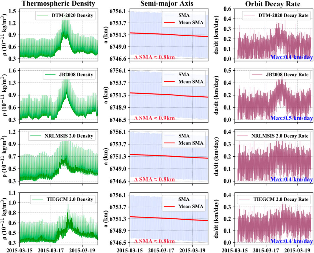
Figure 5. Orbital decay of the Chinese Space Station from March 15th to 19th, 2015, predicted by the HPOP using neutral densities from different thermospheric models (DTM-2020, JB 2008, NRLMSIS 2.0, and TIEGCM 2.0). The left column shows the along-track densities from each model, the middle column presents the SMA and its mean variations under each model, and the right column displays the corresponding decay rates predicted by the respective models.
4.2 Geomagnetic storm on 20 November 2003
During October and November of 2003, record-breaking solar flares and coronal mass ejections were witnessed, which led to severe disturbances in the upper atmosphere and ionosphere of the Earth. This event stands as the most intense geomagnetic storm in solar cycle 23. During this event, the Dst index dropped to −442 nT, and the F10.7 index increased to 171 sfu. Figure 6 illustrates the global distribution of the thermospheric density derived from the four models during different stages of this storm. Analysis of the 2003 geomagnetic storm shows that the global mean thermospheric density increased by 233.8% in DTM-2020, 302.7% in JB 2008, 79.9% in NRLMSIS 2.0, and 153.9% in TIEGCM 2.0 when comparing the main phase to quiet-time conditions.
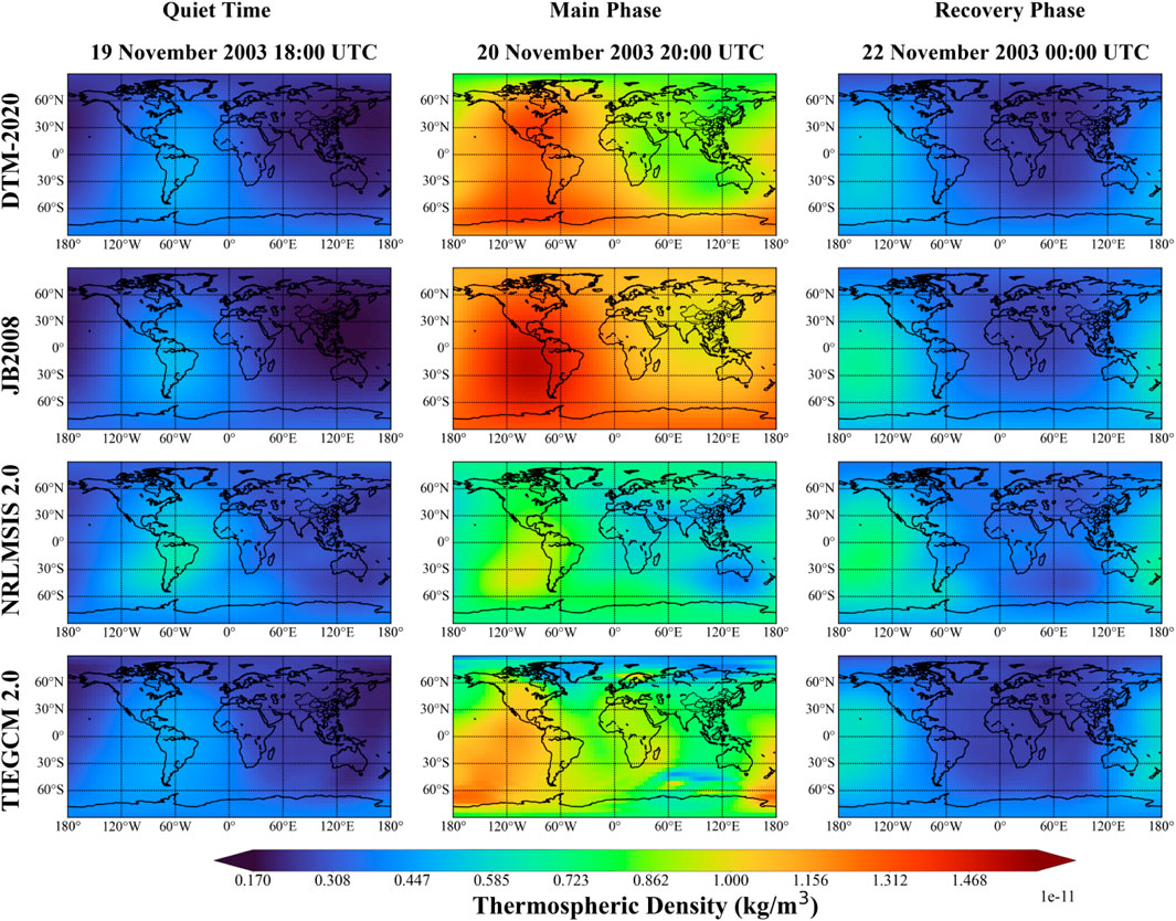
Figure 6. Global thermospheric density distributions at 400 km during the 20 Nov 2003 magnetic storm from different models. The rows correspond to DTM-2020 (top), JB 2008 (second), NRLMSIS 2.0 (third), and TIEGCM 2.0 (bottom), shown across the quiet, main, and recovery phases.
Figure 7 presents a comparative analysis of thermospheric density predictions from four atmospheric models (DTM-2020, JB 2008, NRLMSIS-2.0, and TIEGCM 2.0) against in situ measurements from the CHAMP and GRACE-A satellites during the November 2003 geomagnetic storm. At the CHAMP satellite altitude (380–410 km), all models show significant deviations during the storm’s quiet period, with NRLMSIS-2.0 and TIEGCM 2.0 showing particularly large mean biases (>35%). During the main phase, all models exhibit substantial errors reaching up to 200% in some cases, with error magnitudes comparable to those reported for JB2008 by Oliveira et al. (2020). Among these models, DTM-2020 and JB2008 demonstrate relatively better predictive performance, achieving mean errors of 23.8% and 27.1% respectively, while the other two models maintain consistently high error levels. Consistent with Oliveira et al. (2021) findings of JB2008s systematic underestimation (average 20%) during storm main phases, our results show DTM-2020 and JB2008 have relatively better performance (23.8% and 27.1% respectively). In the recovery phase, DTM-2020 and JB2008 retained their comparative advantage, though all models still exhibited errors exceeding 20%.
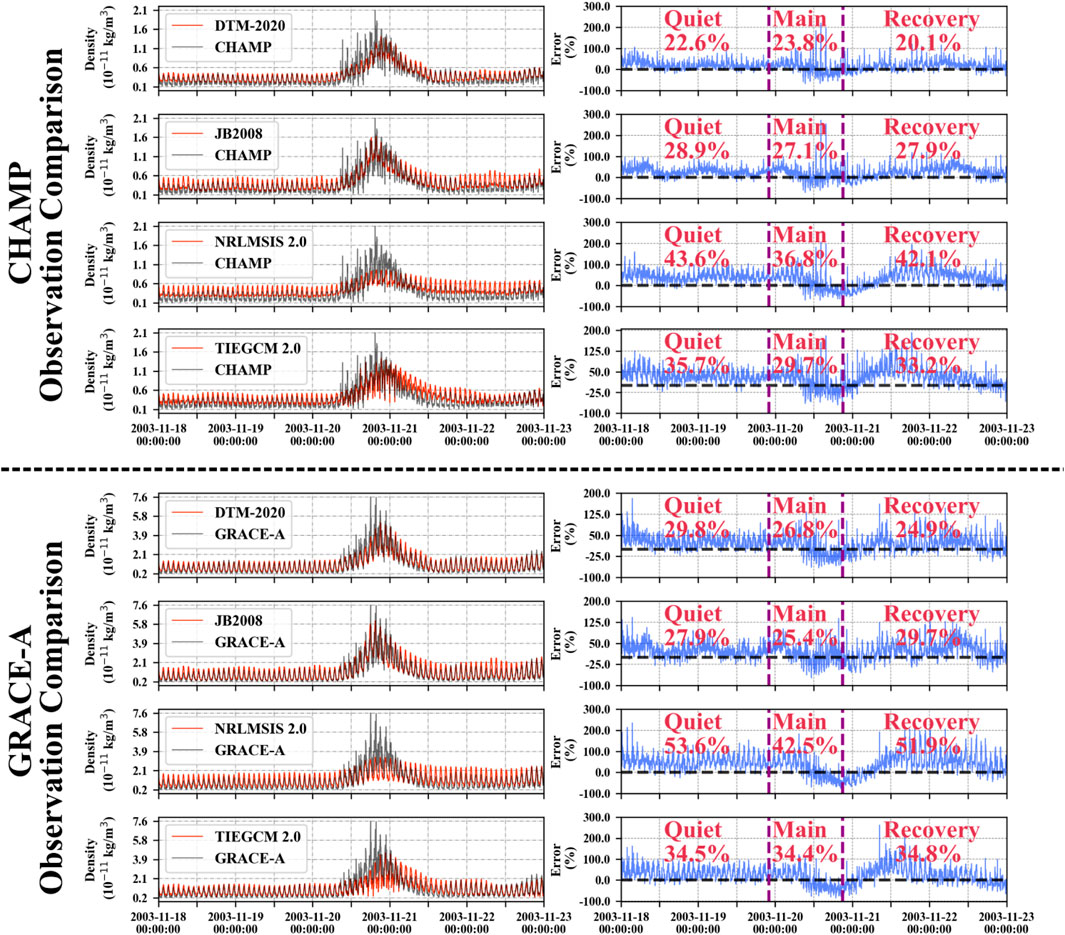
Figure 7. Comparison of the along-track density observed by satellites (CHAMP and GRACE-A) and predicted by DTM-2020, JB 2008, NRLMSIS 2.0, and TIEGCM 2.0 models between March 18th and 23rd, 2003.
For GRACE-A (475–510 km), JB2008 and DTM-2020 consistently outperformed the other models, particularly during the main phase, where their errors remained near 25% and captured the density perturbations more accurately. In contrast, NRLMSIS 2.0 systematically underestimated thermospheric density throughout the event, with errors exceeding 50% during the recovery phase. TIEGCM 2.0 maintaining errors of about 30% across all storm phases.
In general, all tested models exhibit obvious density overestimation during the recovery phase at both CHAMP and GRACE altitudes as shown in Figure 7. The percentage error during the recovery phase is less than 25% for DTM 2020, while that for NRLMSIS 2.0 is over 40% for this particular event. This persistent density overestimation could be due to the lack of NO molecules, which is an important cooling agent (Knipp et al., 2017; Oliveira et al., 2021).
Figure 8 depicts the orbit decay of the CSS predicted by the HPOP model using different thermospheric models during the 20 November 2003 storm. The total CSS orbit decay over the 5-day period is shown in the second column, ranging from 0.7 km to 1.1 km between November 18th and 23rd. The ODRs, shown as burgundy lines, were approximately 0.15 km/day during quiet conditions. During the main phase of this geomagnetic storm, the maximum ODR of the CSS increased to 0.4–0.6 km/day, which is more than twice the rate during the quiet period.
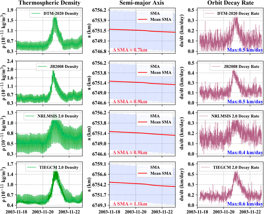
Figure 8. Orbital decay of the Chinese Space Station from March 18th to 23rd, 2003, predicted by the HPOPusing neutral densities from different thermospheric models (DTM-2020, JB 2008, NRLMSIS 2.0, and TIEGCM 2.0). The left column shows the along-track densities from each model, the middle column presents the SMA and its mean variations under each model, and the right column displays the corresponding decay rates predicted by the respective models.
4.3 Geomagnetic storm on 14 March 1989
The March 1989 storm event, which is the most severe geomagnetic storm of the space age, is renowned for its dramatic and unprecedented impact on Earth’s technological systems. It caused a blackout of the Hydro-Québec power grid in Canada, lasting several hours, and resulted in significant economic losses (Bolduc, 2002; Kappenman, 2006; Pulkkinen et al., 2017). From March 6th to 18th, 1989, the rotation of the Sun brought active region 5,395 facing the Earth. During this period, the Sun erupted multiple X-class flares, including an X15-class flare on March 6th. These flares were accompanied by several coronal mass ejections. On March 13th at 01:27 UT, ground-based magnetometers recorded a sudden jump in the magnetic field, signaling the arrival of an interplanetary coronal mass ejection. Over the next 2 days, a large magnetic storm and multiple substorms occurred with the Dst index dropping to −598 nT. As shown in Figure 9, among the density models, the results from NRLMSIS 2.0 show the largest density changes. It should be noted that the required indices for JB2008 are not available for 1989, and therefore this model is not included in the analysis of this event. Compared to the empirical models, the result from TIEGCM 2.0 model does not exhibit much enhancement during the recovery phase. Analysis of the 1989 geomagnetic storm reveals that the percentage increases of the global mean thermospheric density between main phase and quiet time are 144.1% (DTM-2020), 169.3% (NRLMSIS 2.0) and 115.5% (TIEGCM 2.0). Due to the lack of observational data, it is impossible to evaluate the performance of each model during this event.
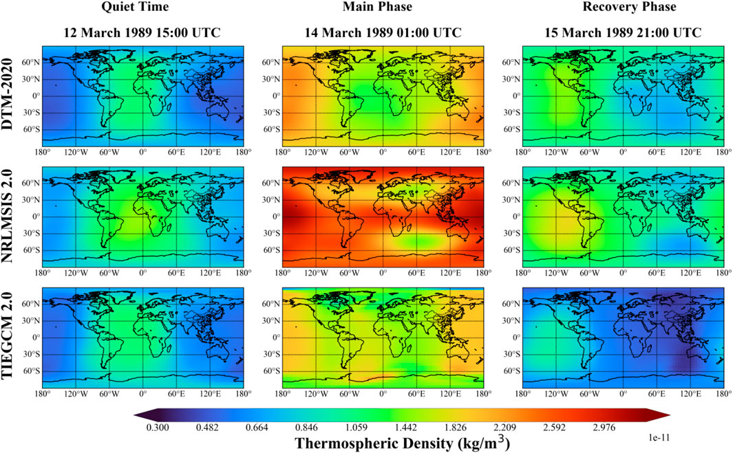
Figure 9. Global thermospheric density distributions at 400 km during the 11 March 1989 magnetic storm from different models. The rows correspond to DTM-2020 (top), NRLMSIS 2.0 (second), and TIEGCM 2.0 (bottom), shown across the quiet, main, and recovery phases.
The drag effect on the CSS during the 1989 event, based on different density models, is shown in Figure 10. The total mean SMA decay is estimated to range from 1.8 km to 2.6 km between March 11th and 16th. The ODR during the quiet period was 0.3 km/day, much higher than the value of 0.15 km/day in the previous two storm events. This difference is probably due to enhanced solar background radiation. The 81-day averaged F10.7 index for this event was about 200 sfu, much higher than the 140 sfu in the 2003 event and 130 sfu in the 2015 event. During the main phase, the maximum ODR for the CSS was estimated by various models to be between 0.8 and 1.1 km/day. This level of decay poses a significant threat to the on-orbit safety of the space station.
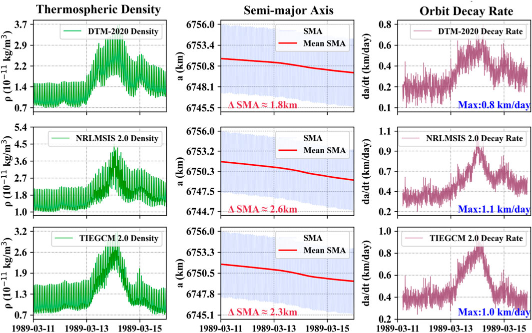
Figure 10. Orbital decay of the Chinese Space Station from March 11th to 16th, 1989, predicted by the HPOP using neutral densities from different thermospheric models (DTM-2020, NRLMSIS 2.0, and TIEGCM 2.0). The left column shows the along-track densities from each model, the middle column presents the SMA and its mean variations under each model, and the right column displays the corresponding decay rates predicted by the respective models.
5 Disscussion
In this study, various thermospheric models are used to estimate the neutral density during the most intense storm events in the previous three solar cycles including the DTM-2020, JB 2008, NRLMSIS 2.0 and TIEGCM 2.0 models. Table 2 shows the storm enhancement in different thermospheric models compared with Swarm, CHAMP, and GRACE observations. The results indicate that the JB2008 model outperforms other models in reproducing thermospheric density enhancements during the extreme magnetic storms of 2003 and 2015. Model error comparisons in Figures 4, 7, based on Swarm, GRACE and CHAMP satellite observations, show that DTM-2020 and JB2008 provides the best peak density simulation for the 2015 and 2003 events. Other models tend to underestimate peak values, which is consistent with the conclusions of Bruinsma and Laurens (2024).
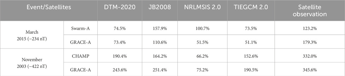
Table 2. Along-track density enhancements relative to quiet-time conditions, derived from different thermospheric models and observations for Swarm-A, CHAMP, and GRACE-A during the March 2015 and November 2003 storm events.
DTM-2020 performs better in estimating peak densities during extreme events. It is worth noting that the DTM limits the maximum ap60 input to 657. In the 1989 event, ap60 exceeded the DTM-2020 model’s limit of 657, reaching 705, which caused DTM to underestimate density changes relative to other models. Therefore, extra caution should be exercised when using DTM for future extreme storm events.
Another notable finding is that the TIEGCM 2.0 model significantly underestimates thermospheric density during the main phase of the 2015 storm. This underestimation was also observed in other extreme events (e.g., 10 May 2024) and may have resulted from insufficient energy input at high latitudes as well as the influence of the nitric oxide (NO) cooling mechanism.
NRLMSIS 2.0 exhibited limited predictive capability for these extreme cases. However, according to Bruinsma and Laurens (2024), NRLMSISE-00 is the least biased when applied to multiple-peak storms. Therefore, it may be a good choice under non-extreme magnetic storm events.
In contrast, the JB2008 model demonstrates remarkable performance advantages during extreme space weather events. Throughout the complete simulation periods of both the 2015 and 2003 extreme events, the model consistently maintained excellent error levels below 30%. Compared to other models that exhibit localized accuracy fluctuations, JB2008 shows superior robustness.The model’s outstanding performance likely stems from its unique input parameter system, which integrates multiple solar radiation indices (F10.7, S10.7, M10.7, Y10.7) with geomagnetic activity parameters (Dst and ap indices), establishing a coupled mechanism for multi-scale energy driving. This multi-parameter architecture enables the model to more accurately capture disturbance characteristics across different energy layers and to effectively respond to nonlinear effects under extreme conditions. However, the requirement for multiple input parameters limits the applicability of JB2008 for real-time orbit prediction.
In summary, considering the input parameter limitations of the DTM-2020 model and the insufficient performance of TIEGCM 2.0 in energy input, the increase in thermospheric density presented by the NRLMSIS 2.0 model may be more reasonable than other models for this specific space weather event in 1989. However, it should be noted that current thermospheric models still exhibit significant prediction errors under extreme geomagnetic conditions, with error levels generally exceeding 20%. A primary factor contributing to this limitation is the scarcity of extreme geomagnetic event samples, which severely constrains the model optimization process. In particular, accurately characterizing energy injection mechanisms and the dynamic response during intense magnetic storms remains a major challenge.
Table 3 shows the orbit decay (
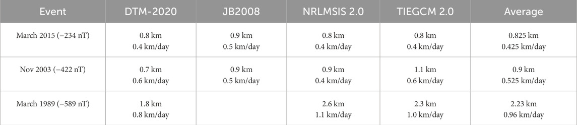
Table 3.
6 Conclusion
The drag impact of extreme space weather events can often lead to sudden safety risks for LEO spacecraft. Therefore, it is important to study the variation of neutral density in LEO orbits and its impact on the orbit decay during extreme storm events. Especially, with the increasing number of spacecraft placed in very low orbits, more attention should be payed to the maintenance and maneuvering of orbits during extreme events. This paper takes CSS as an example to analyze the drag impact during the most severe geomagnetic storms in the previous solar cycles 22, 23, and 24. The CSS, which was completed in 2022, is designed for a lifetime of 10–15 years. With the solar maximum approaching in year 2025, CSS is confronting threats from extreme space weather events. To estimate the possible drag effects due to thermospheric density enhancements, various models are used in this study to simulate the density variations along CSS tracks. These three events occurred in March 1989 November 2003, and March 2015, with minimum Dst indices of −589 nT, −422 nT and −234 nT, respectively. Empirical models (DTM-2020, JB 2008, and NRLMSIS 2.0) and a first-principle model (TIEGCM 2.0) are used to provide the thermospheric density, and the orbital decay is using the HPOP model.
The neutral densities estimated from various thermospheric models (DTM-2020, JB 2008, NRLMSIS 2.0 and TIEGCM 2.0) during these extreme events demonstrate strong enhancement during the main phases. The performance of each model varies for different extreme events, with no single model consistently outperforming the others in all cases. The DTM model performs well in capturing peak density values. However, its effectiveness is limited by the maximum allowable ap60 input index, which is 657. Therefore, extra caution should be exercised when using DTM for future extreme storm events. The comprehensive performance of JB2008 is the best among these models, but it still has at least 20% error with the actual observation. The NRLMSIS 2.0 model exhibits inconsistent performance under extreme geomagnetic conditions, occasionally yielding accurate predictions but often deviating significantly from observations. TIEGCM 2.0 model might have the problem of underestimating the thermosphere density in extreme cases, which may be caused by insufficient energy input at high latitudes. Therefore, in spacecraft operation management, a combination of multiple density models might be considered, along with the potential underestimation during the main phase and overestimation during the recovery phase.
The drag effects on the CSS during the strongest magnetic storm events of solar cycles 24, 23, and 22 are simulated, with orbital decay ranges of 0.8–0.9 km, 0.7–1.1 km, and 1.8–2.3 km, respectively. The maximum orbital decay rates of the different models in the magnetic storms range from 0.4 to 0.5 km/day, 0.4–0.6 km/day, and 0.8–1.1 km/day, respectively, which are about 233%, 300%, and 266% higher than those of the quiet period (0.15 km/day, 0.15 km/day, 0.3 km/day). Although some spacecraft parameters have certain precision limitations, resulting in deviations between their absolute values and the actual values, the trend of their relative decay rate still possesses high reference value and confidence. Spacecraft operators should be aware of the orbital decay rates during quiet periods across years with varying levels of solar radiation activity. For example, the decay rate during a quiet period in 1989 is approximately 0.3 km/day due to the enhanced background solar radiation, while the maximum ODR during a major geomagnetic storm in 2015 ranges from 0.4 to 0.5 km/day. Extra attention should be paid to geomagnetic storms in years of high solar activity, when the increase of the background density will lead to stronger orbital decay. This study might serve as a reference for possible extreme magnetic storm events in the upcoming solar maximum years.
Data availability statement
The original contributions presented in the study are included in the article/supplementary material, further inquiries can be directed to the corresponding author.
Author contributions
KZ: Conceptualization, Data curation, Formal Analysis, Methodology, Software, Validation, Visualization, Writing – original draft, Writing – review and editing. YH: Conceptualization, Funding acquisition, Investigation, Methodology, Project administration, Resources, Supervision, Writing – review and editing. FW: Conceptualization, Resources, Supervision, Writing – review and editing. PZ: Conceptualization, Investigation, Supervision, Validation, Writing – review and editing. HY: Data curation, Resources, Software, Writing – review and editing. JJ: Resources, Writing – review and editing. ZC: Resources, Writing – review and editing.
Funding
The author(s) declare that financial support was received for the research and/or publication of this article. This work is jointly supported by National Key Research and Development Program of China (Grant No. 2022YFF0503904), the National Natural Science Foundation of China (Grant No. 42130210), Guangdong Basic and Applied Basic Research Foundation (Grant No. 2023B1515040021), Shenzhen Science and Technology Program (Grant No. JCYJ20220818102401003) and Shenzhen Key Laboratory Launching Project (Grant No. ZDSYS20210702140800001).
Acknowledgments
We greatly acknowledge European Space Agency (ESA), and the National Geophysical Data Center (NOAA) for providing the data necessary to carry out this work. We thank, U.S. Naval Research Laborat to provide NRLMSIS series model. We also appreciate National Center for thermospheric Research (NCAR) High Altitude Observatory team providing TIEGCM 2.0 model. And the Centre National d’Etudes Spatiales (CNES) providing DTM-2020 model. Thank the author of JB2008 model for open source. The authors gratefully acknowledge the China Manned Space Engineering Office for providing the relevant orbital data used in this study.
Conflict of interest
Author ZC was employed by China Mobile Construction Co., Ltd.
The remaining authors declare that the research was conducted in the absence of any commercial or financial relationships that could be construed as a potential conflict of interest.
Generative AI statement
The author(s) declare that no Generative AI was used in the creation of this manuscript.
Any alternative text (alt text) provided alongside figures in this article has been generated by Frontiers with the support of artificial intelligence and reasonable efforts have been made to ensure accuracy, including review by the authors wherever possible. If you identify any issues, please contact us.
Publisher’s note
All claims expressed in this article are solely those of the authors and do not necessarily represent those of their affiliated organizations, or those of the publisher, the editors and the reviewers. Any product that may be evaluated in this article, or claim that may be made by its manufacturer, is not guaranteed or endorsed by the publisher.
References
Adams, K., Bregou, E., Hudson, M., Kress, B., and Selesnick, R. (2025). Turnover in gleissberg cycle dependence of inner zone proton flux. Space weather. 23 (3), e2024SW004238. doi:10.1029/2024sw004238
Balan, N., Skoug, R., Tulasi Ram, S., Rajesh, P. K., Shiokawa, K., Otsuka, Y., et al. (2014). CME front and severe space weather. J. Geophys. Res. Space Phys. 119 (10). doi:10.1002/2014JA020151
Berger, T. E., Holzinger, M. J., Sutton, E. K., and Thayer, J. P. (2020). Flying through uncertainty. Space weather. 18, e2019SW002373. doi:10.1029/2019SW002373
Berger, T., Dominique, M., Lucas, G., Pilinski, M., Ray, V., Sewell, R., et al. (2023). The thermosphere is a drag: the 2022 starlink incident and the threat of geomagnetic storms to low Earth orbit space operations. Space weather. 21 (3), e2022SW003330. doi:10.1029/2022SW003330
Bolduc, L. (2002). GIC observations and studies in the hydro-québec power system. J. Atmos. Solar-Terrestrial Phys. 64 (16), 1793–1802. doi:10.1016/S1364-6826(02)00128-1
Bowman, B. R., Marcos, F. A., Moe, K., and Moe, M. M. (2007). “Determination of drag coefficient values for CHAMP and GRACE satellites using orbit drag analysis,” in Paper AAS 07-259. San Diego, CA: American Astronautical Society Publications Office.
Briden, J., Clark, N., Siew, P. M., Linares, R., and Fang, T. W. (2022). “Impact of space weather on space assets and satellite launches,” in Proceedings of the 23rd advanced maui optical and space surveillance technologies. Maui, Hawaii, United States, 1–22.
Bruinsma, S., and Boniface, C. (2021). The operational and research DTM-2020 thermosphere models. J. Space Weather Space Clim. 11, 47. doi:10.1051/swsc/2021032
Bruinsma, S., and Laurens, S. (2024). Thermosphere model assessment for geomagnetic storms from 2001 to 2023. J. Space Weather Space Clim. 14, 28. doi:10.1051/swsc/2024027
Bruinsma, S., Boniface, C., Sutton, E. K., and Fedrizzi, M. (2021). Thermosphere modeling capabilities assessment: geomagnetic storms. J. Space Weather Space Clim. 11, 12. doi:10.1051/swsc/2021002
Chen, G.-m., Xu, J., Wang, W., and Burns, A. G. (2014). A comparison of the effects of CIR- and CME-Induced geomagnetic activity on thermospheric densities and spacecraft orbits: statistical studies. J. Geophys. Res. Space Phys. 119 (9), 7928–7939. doi:10.1002/2014JA019831
Dang, T., Li, X., Luo, B., Li, R., Zhang, B., Pham, K., et al. (2022). Unveiling the space weather during the Starlink satellites destruction event on 4 February 2022. Space weather. 20 (8), e2022SW003152. doi:10.1029/2022SW003152
DeLucas, L. J. (1996). International space station. Acta astronaut. 38 (4-8), 613–619. doi:10.1016/0094-5765(96)00056-2
Dickinson, R. E., Ridley, E. C., and Roble, R. G. (1981). A three-dimensional general circulation model of the thermosphere. J. Geophys. Res. Space Phys. 86 (A3), 1499–1512. doi:10.1029/JA086iA03p01499
Eckstein, M., and Hechler, F. (1970). “A reliable derivation of the perturbations due to any zonal and tesseral harmonics of the geopotential for nearly-circular satellite orbits, Scientific Report ESRO SR-13, European Space Research, Organization,”. Darmstadt, Germany: Federal Republic of Germany.
Elvidge, S., Godinez, H. C., and Angling, M. J. (2016). Improved forecasting of thermospheric densities using multi-model ensembles. Geosci. Model Dev. 9 (6), 2279–2292. doi:10.5194/gmd-9-2279-2016
Emmert, J. T. (2015). Thermospheric mass density: a review. Adv. Space Res. 56 (5), 773–824. doi:10.1016/j.asr.2015.05.038
Emmert, J. T., Drob, D. P., Picone, J. M., Siskind, D. E., Jones, M., Mlynczak, M. G., et al. (2020). NRLMSIS 2.0: a whole atmosphere empirical model of temperature and neutral species densities. Earth Space Sci. 7, e2020EA001321. doi:10.1029/2020EA001321
Feynman, J., and Ruzmaikin, A. (2014). The Centennial gleissberg cycle and its association with extended minima. J. Geophys. Res. Space Phys. 119 (8), 6027–6041. doi:10.1002/2013JA019478
Gleissberg, W. (1965). The eighty-year solar cycle in auroral frequency numbers. J. Br. Astron. Assoc. 75, 227–231.
Gu, Y. (2022). The China space station: a new opportunity for space science. Natl. Sci. Rev. 9 (1), nwab219. doi:10.1093/nsr/nwab219
He, C., Yang, Y., Carter, B., Kerr, E., Wu, S., Deleflie, F., et al. (2018). Review and comparison of empirical thermospheric mass density models. Prog. Aerosp. Sci. 103, 31–51. doi:10.1016/j.paerosci.2018.10.003
Heelis, R. A., Lowell, J. K., and Spiro, R. W. (1982). A model of the highlatitude ionospheric convection pattern. J. Geophys. Res. Space Phys. 87, 6339–6345. doi:10.1029/JA087iA08p06339
Kappenman, J. G. (2006). Great geomagnetic storms and extreme impulsive geomagnetic field disturbance events - an analysis of observational evidence including the great storm of may 1921. Adv. Space Res. 38 (2), 188–199. doi:10.1016/j.asr.2005.08.055
Kaula, W. M., and Street, R. E. (1967). Theory of satellite geodesy: applications of satellites to geodesy. Cour. Corp. 20 (10), 101. doi:10.1063/1.3033941
Kilpua, E. K. J., Fontaine, D., Moissard, C., Ala-Lahti, M., Palmerio, E., Yordanova, E., et al. (2019). Solar wind properties and geospace impact of coronal mass ejection-driven sheath regions: variation and driver dependence. Space weather. 17, 1257–1280. doi:10.1029/2019SW002217
Knipp, D. J., Pette, D. V., Kilcommons, L. M., Isaacs, T. L., Cruz, A. A., Mlynczak, M. G., et al. (2017). Thermospheric nitric oxide response to shock-led storms. Space weather. 15 (2), 325–342. doi:10.1002/2016SW001567
Krauss, S., Temmer, M., Veronig, A., Baur, O., and Lammer, H. (2015). Thermospheric and geomagnetic responses to interplanetary coronal mass ejections observed by ACE and GRACE: statistical results. J. Geophys. Res. 120, 8848–8860. doi:10.1002/2015JA021702
Lakhina, G. S., and Tsurutani, B. T. (2017). Satellite drag effects due to uplifted oxygen neutrals during super magnetic storms. Nonlinear Process. Geophys. 24 (4), 745–750. doi:10.5194/npg-24-745-201
Lechtenberg, T., McLaughlin, C. A., Locke, T., and Krishna, D. M. (2013). Thermospheric density variations: observability using precision satellite orbits and effects on orbit propagation. Space Weather. 11 (1), 34–45. doi:10.1029/2012SW000848
Li, Y., Zhu, G., Qin, G., Tang, P., and He, Y. (2014). Significant differences of thermosphere density between the model and the obvervation values during different altitudes and geomagnetic disturbances. Chin. J. Geophys. 57 (11), 3703–3714.
Liu, W. (2015). Analysis of satellite drag coefficient based on wavelet transformation. J. Astronautics 36 (2), 142. doi:10.1016/j.jsse.2020.07.018
Oliveira, D. M., and Zesta, E. (2019). Satellite orbital drag during magnetic storms. Space weather. 17 (11), 1510–1533. doi:10.1029/2019SW002287
Oliveira, D. M., Zesta, E., Hayakawa, H., and Bhaskar, A. (2020). Estimating satellite orbital drag during historical magnetic superstorms. Space weather. 18 (11), e2020SW002472. doi:10.1029/2020SW002472
Oliveira, D. M., Zesta, E., Mehta, P. M., Licata, R. J., Pilinski, M. D., Kent Tobiska, W., et al. (2021). The current state and future directions of modeling thermosphere density enhancements during extreme magnetic storms. Front. Astronomy Space Sci. 8 (764144), 764144. doi:10.3389/fspas.2021.764144
Park, R. S., Folkner, W. M., Williams, J. G., and Boggs, D. H. (2021). The JPL planetary and lunar ephemerides DE440 and DE441. Astronomical J. 161 (3), 105. doi:10.3847/1538-3881/abd414
Picone, J. M., Hedin, A. E., Drob, D. P., and Aikin, A. C. (2002). NRLMSISE-00 empirical model of the atmosphere: statistical comparisons and scientific issues. J. Geophys. Res. Space Phys. 107 (A12), SIA–15. doi:10.1029/2002JA009430
Prieto, D. M., Graziano, B. P., and Roberts, P. C. E. (2014). Spacecraft drag modelling. Prog. Aerosp. Sci. 64, 56–65. doi:10.1016/j.paerosci.2013.09.001
Prölss, G. W. (2011). Density perturbations in the upper atmosphere caused by the dissipation of solar wind energy. Surv. Geophys. 32 (2), 101–195. doi:10.1007/s10712-010-9104-0
Pulkkinen, A., Bernabeu, E., Thomson, A., Viljanen, A., Pirjola, R., Boteler, D., et al. (2017). Geomagnetically induced currents: science, engineering, and applications readiness. Space weather. 15 (7), 828–856. doi:10.1002/2016SW001501
Qian, L., and Solomon, S. C. (2012). Thermospheric density: an overview of temporal and spatial variations. Space Sci. Rev. 168 (1), 147–173. doi:10.1007/s11214-011-9810-z
Qian, L., Burns, A. G., Emery, B. A., Foster, B., Lu, G., Maute, A., et al. (2014). The NCAR TIEGCM: a community model of the coupled thermosphere/ionosphere system. In J. Huba, R. Schunk, and G. Khazanov Modeling the ionosphere-thermosphere system, (201). Washington, DC: Geophysical Monograph Series is the American Geophysical Union (AGU).
Refaat, A., Badawy, A., Ashry, M., and Omar, A. (2018). “High accuracy spacecraft orbit propagator validation,” in The international conference on applied mechanics and mechanical engineering vol. 18, no. 18th international conference on applied mechanics and mechanical engineering. (Cairo, Egypt: Military Technical College), 1–9.
Ren, D., and Lei, J. (2023). Two-line elements based thermospheric mass density specification from parameter optimization of a physics-based model. Space weather. 21 (9), e2023SW003553. doi:10.1029/2023SW003553
Richmond, A. D., Ridley, E. C., and Roble, R. G. (1992). A thermosphere/ionosphere general circulation model with coupled electrodynamics. Geophys. Res. Lett. 19 (6), 601–604. doi:10.1029/92GL00401
Roble, R. G., Ridley, E. C., Richmond, A. D., and Dickinson, R. E. (1988). A coupled thermosphere/ionosphere general circulation model. Geophys. Res. Lett. 15 (12), 1325–1328. doi:10.1029/GL015i012p01325
Sivolella, D. (2022). “Space shuttle and skylab: a missed opportunity,” in The untold stories of the space shuttle program: unfulfilled dreams and missions that never flew (Cham: Springer International Publishing), 244–270.
Spiridonova, S., Kirschner, M., and Hugentobler, U. (2014). “Precise mean orbital elements determination for LEO monitoring and maintenance,” in 24th international symposium on space flight dynamics. Laurel, Maryland, USA. Available online at: https://elib.dlr.de/103814/.
Tapley, B., Ries, J., Bettadpur, S., Chambers, D., Cheng, M., Condi, F., et al. (2007). The GGM03 mean Earth gravity model from GRACE. AGU Fall Meet. Abstr. 2007, G42A-03.
Thirsk, R., Kuipers, A., Mukai, C., and Williams, D. (2009). The space-flight environment: the International Space Station and beyond. Cmaj. 180 (12), 1216–1220. doi:10.1503/cmaj.081125
Vallado, D. A. (2001). Fundamentals of Astrodynamics and Applications. Berlin, Heidelberg, Germany: Springer Science & Business Media.
Weimer, D. R. (2005). Improved ionospheric electrodynamic models and application to calculating Joule heating rates. J. Geophys. Res. Space. Phys. 110 (A5). doi:10.1029/2004JA010884
Ya-Ying, L., and Zhao, C. (1995). An analysis of the influence of various atmospheric models on the drift and lifetime of a space station. Acta Astronaut. 35 (2-3), 99–105. doi:10.1016/0094-5765(94)00155-F
Yamazaki, Y., Matzka, J., Stolle, C., Kervalishvili, G., Rauberg, J., Bronkalla, O., et al. (2022). Geomagnetic activity index hpo. Geophys. Res. Lett. 49 (10), e2022GL098860. doi:10.1029/2022GL098860
Zesta, E., and Huang, C. Y. (2016). “Satellite orbital drag,” in Space weather fundamentals. (Boca Raton, FL, United States: CRC Press), 329–351.
Keywords: thermospheric density, geomagnetic storm, orbit decay, space weather, china space station
Citation: Zhang K, Huang Y, Wei F, Zuo P, Yang H, Ji J and Chen Z (2025) Thermospheric density variations during extreme geomagnetic storms and their potential impact on the orbit of the China space station. Front. Astron. Space Sci. 12:1644152. doi: 10.3389/fspas.2025.1644152
Received: 10 June 2025; Accepted: 17 September 2025;
Published: 02 October 2025.
Edited by:
Tzu-Wei Fang, Space Weather Prediction Center (NOAA), United StatesReviewed by:
Octav Marghitu, Space Science Institute, RomaniaDenny Oliveira, University of Maryland, United States
Copyright © 2025 Zhang, Huang, Wei, Zuo, Yang, Ji and Chen. This is an open-access article distributed under the terms of the Creative Commons Attribution License (CC BY). The use, distribution or reproduction in other forums is permitted, provided the original author(s) and the copyright owner(s) are credited and that the original publication in this journal is cited, in accordance with accepted academic practice. No use, distribution or reproduction is permitted which does not comply with these terms.
*Correspondence: Yanshi Huang, aHVhbmd5YW5zaGlAaGl0LmVkdS5jbg==