Novel method and tool to identify solitary waves in the Martian plasma environment

This paper introduces a method and an innovative graphical user interface (GUI) tool to identify bipolar solitary wave structures in the Mars Atmosphere and Volatile EvolutioN (MAVEN) mission dataset. As input to this tool, we utilized medium-frequency burst mode calibrated electric field data obtained from the Langmuir Probe and Waves (LPW) instrument aboard MAVEN. To detect solitary waves, we first discuss the typical theoretical solitary wave structure and its key features. Based on these features, we developed a series of mathematical conditions that are applied to the LPW electric field dataset. After rigorous testing, a MATLAB executable GUI application named SWIT (Solitary Wave Identifying Tool) was developed. The output of SWIT provides the amplitude, width, and time of occurrence of the solitary waves. Furthermore, we evaluate the accuracy and limitations of SWIT. It is found that SWIT demonstrates high efficiency. It is a dedicated identifier for analyzing medium-frequency electric field measurements from the MAVEN spacecraft to search for solitary wave structures in the Martian plasma environment. It is suggested that this novel method can be applied to datasets from different spacecraft in other planetary plasma environments with minor modifications.

1 Introduction

Electrostatic solitary waves (ESWs) are nonlinear, isolated electric field pulses observed in space plasmas. These waves typically propagate along the direction of the magnetic field and exhibit negligible fluctuations in the perpendicular component of the magnetic field. They were first detected in auroral plasma by the S3-3 polar-orbiting satellite (Temerin et al., 1982). Later, high-resolution electric field measurements from the Geotail spacecraft revealed that broadband electrostatic noise (BEN) consists of isolated bipolar solitary structures (Matsumoto et al., 1994). Since then, ESWs have been observed in various regions of the Earth’s magnetosphere, such as the auroral zone (Ergun et al., 1998; Pickett et al., 2004), magnetopause (Cattell et al., 2002; Graham et al., 2015; Graham et al., 2016), magnetosheath (Pickett et al., 2003; Holmes et al., 2018; Shaikh et al., 2024), bow shock (Hobara et al., 2008; Wang et al., 2014; Vasko et al., 2018; Vasko et al., 2020; Sun et al., 2022; Kamaletdinov et al., 2022), plasma sheet (Ergun et al., 2009; Tong et al., 2018; Mozer et al., 2018; Wang et al., 2022), magnetotail (Norgren et al., 2015), inner magnetosphere (Vasko et al., 2017a), dusk flank region (Arya and Kakad, 2025), and so on. As new observations continue to emerge, theoretical (Singh and Lakhina, 2001; Pickett et al., 2005; Kakad et al., 2007; Lakhina et al., 2008a; Lakhina et al., 2008b, 2009; Kakad et al., 2009; Lakhina et al., 2011a; Lakhina et al., 2011b; Olivier et al., 2015; Maharaj et al., 2015; Kakad et al., 2016; Singh et al., 2024) and simulation (Omura et al., 1996; Umeda et al., 2002; Kakad et al., 2013; Kakad et al., 2014; Lotekar et al., 2016; Kakad A. et al., 2017; Lotekar et al., 2017; Vasko et al., 2017b; Dillard et al., 2018; Lotekar et al., 2019; Kakad and Kakad, 2019) studies have been conducted to investigate their generation mechanisms. In general, monopolar (double layer), bipolar, and occasionally observed tripolar structures fall under the ESW category. In this paper, the term solitary waves refers specifically to bipolar solitary structures.

In fluid models, ESWs can be classified as ion or electron acoustic solitary waves (IASWs/EASWs), depending on the dominant driving species. EASWs exhibit phase velocities of a few thousand kilometers per second, whereas IASWs typically have phase velocities of a few hundred kilometers per second. A review article on ESWs as acoustic soliton models is provided by Lakhina et al. (2021). In kinetic models, ESWs are interpreted as ion or electron holes in phase space, depending on the polarity of the associated potential structures (Eliasson and Shukla, 2006; Aravindakshan et al., 2018a; Aravindakshan et al., 2018b, Aravindakshan et al., 2020; Aravindakshan et al., 2021; Aravindakshan et al., 2023). In space plasmas, they play a role in the acceleration, heating, energy dissipation, and trapping of charged particles (Ergun et al., 2004; Andersson and Ergun, 2012; Mozer et al., 2013; Kakad et al., 2017a; Kakad et al., 2017b; Wang et al., 2023).

ESWs are not confined to Earth’s plasma environment; they have also been observed in the Martian magnetosheath (Kakad et al., 2022; Thaller et al., 2022; Pandey et al., 2025a; Pandey et al., 2025c), the Venusian plasma environment (Malaspina et al., 2020), and Saturn’s magnetosphere (Williams et al., 2006). By studying the ambient plasma parameters, various generation mechanisms have been proposed for the ESWs (Singh et al., 2022; Rubia et al., 2023; Varghese et al., 2024a; Varghese et al., 2024b). In case of Mars, in recent studies the ESWs have been reported using the electric field data from Langmuir Probe and Waves (LPW) instrument aboard the Mars Atmosphere and Volatile Evolution (MAVEN) mission. However, ESWs on Mars have not been studied as extensively as those on Earth. The LPW instrument measures the y-component of the electric field in the spacecraft’s coordinate system (Andersson et al., 2015). Therefore, limited information is available about the propagation of ESWs. A statistical study of ESWs would provide valuable insights into their occurrence in the plasma environment of an unmagnetized planet like Mars, helping to understand their role in particle dynamics. However, manual detection of solitary waves from such a large dataset is a real challenge.

In this paper, we present a tool for identifying bipolar solitary waves from the MAVEN dataset. Previously, Kojima et al. (2000) developed a method to identify ESWs from the Geotail spacecraft dataset. They employed a bit-pattern comparison technique using two sample waveforms of ESWs with opposite polarity. They defined an ESW index that quantifies the deviation from or similarity to the sample waveforms. This process is carried out by shifting the sample waveforms in time to match the observed signals. However, since the width of ESWs in the time domain can vary, different sample waveforms with varying pulse widths are required. Hansel et al. (2021) used the Solitary Wave Detector (SWD) on NASA’s Magnetospheric Multiscale (MMS) mission to map solitary waves in the Earth’s magnetosphere, identifying 60% of all bipolar solitary waves. It is based on a pseudo-standard deviation technique. In the present paper, we use a cumulative-integration-based approach to identify solitary waves. The developed tool is rigorously tested using LPW medium-frequency electric field data from the MAVEN spacecraft, and its efficiency in detecting solitary waves is examined. The paper is organized as follows: the methodology and module sequence in the program are detailed in Sections 2, 3, respectively. The usage and requirements of the Solitary Wave Identifying Tool (SWIT) are elaborated in Section 4. The results are discussed in Section 5. Finally, the study is summarized and concluded in Section 6.

2 Methodology

First, we present the mathematical formulation of a solitary wave and outline its key properties using cumulative integration and first-order differentiation. We examined discrepancies between the ideal and observed solitary wave structures and used this information to ensure accurate identification of solitary waves in the real data. Below, in different subsections, we describe the specific criteria employed in the program to identify solitary waves. We assume the following form for the electric potential linked to the solitary wave structure, as outlined by Kojima et al. (2000) and Krasovsky et al. (1997),

$\varphi \left(x\right)={\varphi }_0\exp \left(-\frac{x^2}{{\lambda }^2}\right)(1)$

where ${\varphi }_0$ is the peak of potential at position $x=0$ and $\lambda$ is the distance where potential falls by $1/e$ times of ${\varphi }_0$. Spacecraft measurements provide electric field data in the time domain rather than the space domain. Therefore, on substituting $x=vt$ in Equation 1 and using $E(x)=-d\varphi /dx$, we get

$E\left(t\right)=-\frac{1}{v}\frac{d\varphi }{dt}=2t{\varphi }_0\frac{v}{{\lambda }^2}\exp \left(-\frac{v^2{t}^2}{{\lambda }^2}\right)(2)$

where $v$ is the magnitude of the phase velocity of the solitary wave and is assumed to be constant.

To reduce parametric dependency and focus on the behavior of the electric field as a function of time, we take $v=1$, $\lambda =1$, and ${\varphi }_0=1$; then Equation 2 becomes,

$E\left(t\right)=2t\exp \left(-t^2\right)(3)$

Equation 3 represents the typical electric field $(E)$ profile of solitary waves associated with positive or negative potential and traveling in either negative or positive $x-$direction. Based on this, we label the electric field profiles, where the negative half-cycle occurs first, followed by the positive half-cycle, as type-1 solitary waves. Conversely, those electric field profiles where the positive half-cycle occurs first, followed by the negative half-cycle, are labeled as type-2 solitary waves. Here, the positive and negative peaks in the solitary wave profile are termed as $E_{+}$ and $E_{-}$, with their corresponding time instances as $t_{+}$ and $t_{-}$, respectively.

An electric field profile of the type-1 solitary waves in the time domain is shown in Figure 1A. Its cumulative integration (CI), defined as $-\int E(t)dt$, is displayed in Figure 1B. It may be noted that the negative sign in CI is used to maintain analogy with the electric potential. The first-order derivative of the electric field profile, $E^{\prime }(t)$, is shown in Figure 1C. The vertical blue dashed lines indicate the instance of $t_{-}$ and $t_{+}$, with their midpoint $(t_c)$ marked by the black dashed line. The vertical red dashed lines indicate the initial $(t_i)$ and final $(t_f)$ instances, where the peak of CI decreases by 99.7%. The width of the solitary wave structure $(\mathrm{\Delta }t)$ is defined as the time interval between $t_{-}$ and $t_{+}$. Here, we list properties of the ideal form of solitary wave based on Figure 1; (i) Equal absolute values of $E_{+}$ and $E_{-}$, (ii) Equal durations of negative and positive half cycle, $d_{-}=d_{+}$ (here $d_{-}=|t_i-t_c|$ and $d_{+}=|t_f-t_c|$), (iii) Continuous increase in the $E(t)$ from $t_{-}$ to $t_{+}$, (iv) In CI profile, no change in sign from time $t_i$ to $t_f$, (v) Single turning point between $t_{-}$ to $t_{+}$ in $E^{\prime }(t)$. Here, the type-1 or type-2 categories are used only for convenience, and they do not signify the polarity of the potential structure associated with the electric field. The polarity of the potential can not be identified unless the direction of propagation of solitary waves is known. We consider all the above-listed properties of the solitary wave while setting different criteria in a MATLAB executable GUI tool named SWIT to identify solitary waves. In reality, the observed solitary wave structure does not follow its exact ideal form. Therefore, while dealing with the data, the properties mentioned above are treated as references and conditionally modified to meet the requirements. The modified conditions and their implementation in the SWIT are discussed in the next Section 3.

Figure 1

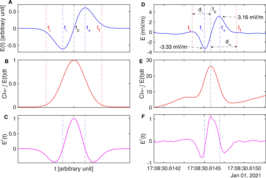
Figure 1. The ideal form of the solitary wave: (A) electric field profile of the solitary wave waveform, (B) cumulative integration (CI) of the solitary wave waveform, and (C) the first-order derivative of the solitary wave waveform are shown as functions of time. Similarly, observation of a solitary wave from the LPW instrument on 1 January 2021: (D) electric field profile, (E) cumulative integration, and (F) first-order derivative are shown as functions of time in UT. In panel (D) $t_i$ and $t_f$ are the initial and final time instances of the solitary wave waveform; $t_{-}$ and $t_{+}$ are the time instances associated with $E_{-}$ and $E_{+}$, respectively, with the midpoint marked by $t_c$; $d_{-}$ and $d_{+}$ represent the durations of the negative and positive half-cycles of the solitary wave, respectively.

As an example, the type-1 solitary wave structure seen in LPW electric field data is displayed in Figure 1D with its CI in panel (E) and first-order derivative in panel (F). We mark the instances $t_i$ and $t_f$ by following the turning points in the electric field before and after the $t_{-}$ and $t_{+}$, respectively. The turning points are the locations where the slope of the curve changes its sign. As far as the first property of the solitary wave structure is concerned, it is unlikely that in real data, we encounter $|E_{+}|=|E_{-}|$. Therefore, we define a symmetry parameter for amplitude as $S_a=min\{|E_{+}|,|E_{-}|\}/max\{|E_{+}|,|E_{-}|\}$. Here, $S_a$ can vary between 0 and 1, and $S_a$ = 1 represents 100% symmetry in amplitudes. We set a minimum acceptable limit on $S_a$ as 0.6. If $S_a$ falls below 0.6, then the bipolar electric field pulse is not treated as solitary wave. In Figure 1D, the absolute positive and negative peaks differ by 0.17$mV/m$ and $S_a$ = 0.95. Hence, it satisfies the acceptance criteria for being selected as solitary wave. Similarly, achieving equal durations for the positive and negative half-cycles is an ideal scenario (i.e., property-2). We defined a symmetry parameter for solitary wave half-cycle duration as $S_d=min\{d_{-},d_{+}\}/max\{d_{-},d_{+}\}$. If $S_d$ exceeds 0.6, then the bipolar pulse is selected. A threshold value of 0.6 was set after visually inspecting many burst datasets. For values greater than 0.6 (such as 0.65 or 0.70), a significant number of solitary wave structures go undetected, even though they could have been identified through visual inspection.

Next, let us discuss the solitary wave properties (iii)-(v). The solitary waves are typically observed in high-resolution electric field data. Between $t_{-}$ and $t_{+}$, a few outliers may disrupt the continuous increase of the electric field, introducing the local irregular slope variations. These variations may not be visually apparent, but they can result in multiple turning points in $E^{\prime }(t)$ within $t_{-}$ and $t_{+}$. To address this issue, the moving average smoothing method is employed. Ideally, one anticipates a single peak in CI associated with the solitary wave. Therefore, we also examined the turning points before and after the peak of the CI. These conditions are elaborated in the next Section 3.

3 Module sequence in SWIT

This subsection describes the logical workflow of different modules in the computer program, emphasizing the significance of each step in the process. For clarity, the explanation focuses solely on type-1 solitary wave, as the logic used to detect the type-2 solitary wave is identical, differing only in sign at specific points. A flowchart illustrating the main structure of the SWIT program is presented in Figure 2. It may be noted that SWIT is developed using MATLAB software.

Figure 2

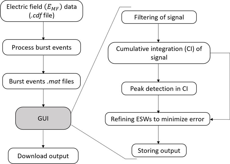
Figure 2. Structure of the program flow used in the development of the SWIT GUI.

3.1 Data loading and filtering

In this study, we use the medium-frequency (100 Hz–32 kHz) burst-mode calibrated electric field data obtained from the LPW instrument onboard MAVEN (Andersson, 2024). The sampling frequency $(f_s)$ is 65,536 Hz, and the duration of a single burst is typically 62.5 ms (4,096 data points) or an integral multiple of this. Initially, using “process_burst_events.m” program file, the user can convert electric field raw data into individual “.mat” files that contain the electric field and time information for each burst event that occurred on a given day. These individual burst files (time and electric field) serve as input to the SWIT module. At this stage, the electric field signal and corresponding time series data for a single burst event get loaded. Additionally, the user must provide the sampling rate of the data in Hz.

A Butterworth bandpass filter is applied to the electric field signal based on the input sampling frequency, with appropriate lower cut-off $(f_{lc})$ and upper cut-off $(f_{hc}<f_s/2)$ frequencies. The lower cut-off frequency $(f_{lc})$ is used to eliminate long-term variations in the signal. Essentially, this process detrends the cumulative integration of a signal. Also, the higher cut-off frequency helps in removing the high-frequency noise. As an example, a series of electric field pulses observed in LPW electric field data on 9 February 2015 are depicted in Figure 3A. We can see that the solitary wave marked with the dashed rectangle exhibits small kinks. The frequency associated with these kinks is significantly higher than the frequencies of the solitary waves. The process of filtering removes these kinks. Figure 3B depicts the filtered signal, where the kinks have been eliminated. The $f_{lc}$ and $f_{hc}$ are chosen to ensure that the overall solitary wave structure of the signal remains largely unaffected. We have selected $f_{lc}=$100 Hz and $f_{hc}=$15 kHz for medium-frequency LPW electric field measurements. Figure 3C depicts the CI for the filtered electric field signal shown in Figure 4B. The use of CI in solitary wave identification is elaborated in the next subsection.

Figure 3

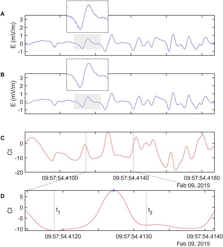
Figure 3. An electric field signal illustrating solitary waves: (A) original data showing solitary waves with small kinks, visible in the zoomed-in view of the grey-shaded region; (B) data after filtering, demonstrating the removal of kinks in the same region; (C) cumulative integration (CI) of the filtered data; (D) a zoomed-in view of the CI peak (marked by an asterisk), highlighting turning points $t_1$ and $t_2$ before and after the peak (see dashed vertical lines).

Figure 4

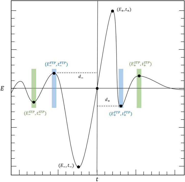
Figure 4. A schematic of the solitary wave waveform, illustrating the allowed ranges for the first and second turning points before $t_{-}$ and after $t_{+}$, aids in formulating the conditions to reduce false positives while detecting solitary waves. The values of the electric field at turning points $t_{\pm }^{\mathit{FTP}}$ and $t_{\pm }^{\mathit{STP}}$ are examined, where the superscripts $FTP$ and $STP$ denote the first and second turning points, respectively. The subscripts $\pm$ indicate positive and negative half-cycles. The permissible range for $FTP$, shown in the blue-shaded region, lies between 0.25 $E_{-}$ and 0.25 $E_{+}$. Similarly, the $STP$ range, represented by the green-shaded region, also lies between 0.25 $E_{-}$ and 0.25 $E_{+}$. These thresholds were determined based on the extensive testing with electric field data.

3.2 Cumulative integration and peak identification

Theoretically, each bipolar electric field pulse of type-1 will give rise to one positive peak in CI. We used this approach to identify the location of likely solitary waves in the observed electric field signal. The CI of the filtered signal is calculated, and the location of several peaks apparent in CI is identified. Each peak in CI corresponds to the center of the respective solitary wave structure (see Figure 3C). A peak in CI is identified if the amplitudes of the five preceding and five following points are smaller and decrease continuously on both sides of the peak. Next, the occurrence of turning points in CI preceding and following such peaks are identified and marked as $t_1$ and $t_2$. As an example, the time variation of CI associated with one solitary wave structure is shown in Figure 3D. The turning points in CI before and after a peak shown with a blue asterisk are marked by vertical dashed black lines. It is noted that the solitary wave structure is located within $t_1$ and $t_2$ only. We estimated $E_{+}$ and $E_{-}$, and if their magnitude exceeds 0.5 mV/m, then that solitary wave structure is considered for further analysis. The resolution of electric field data is 0.3 mV/m; therefore, we chose a limit of 0.5 mV/m as the acceptance criteria for solitary wave structures. In this way, each peak in the CI undergoes similar scrutiny. We ensure that each identified solitary wave structure is well-separated and is not a part of wave oscillations. This is carried out by checking the number of turning points in $E(t)$ between two successive solitary waves identified by the program. If there are two or more turning points between $E_{+}$ of the first solitary wave and $E_{-}$ of the next solitary wave in the case of two successive type-1 solitary waves, such structures will be selected.

It may be noted that a major part of the solitary wave identification is covered by different steps elaborated so far. However, electric field data often possess small amplitude oscillations close to the solitary wave structure. Therefore, solitary waves identified within the turning points obtained in the previous step undergo further refinement to minimize error in the identification of solitary wave. A previously discussed issue involves the presence of multiple turning points in $E^{\prime }(t)$ within the interval from $t_{-}$ to $t_{+}$. To address this, the filtered signal from $t_{-}$ to $t_{+}$ is further smoothed using $n$ points, where $n$ is determined as one-fourth of the signal length between $t_{-}$ and $t_{+}$. This criterion is developed by examining numerous examples of solitary waves. If multiple turning points persist after smoothing, then such solitary waves are rejected. We also examined the values of the electric field signal at its various turning points in and around the solitary wave, as illustrated in the schematic of the solitary wave profile in Figure 4. We check the values of signals at $t_{\pm }^{\mathit{FTP}}$, $t_{\pm }^{\mathit{STP}}$. Here, the superscripts $FTP$ and $STP$ refer to the first and second turning points, respectively. The subscripts $\pm$ represent the positive and negative half-cycle of solitary wave. The ranges for $FTP$ and $STP$, within which the values must fall, are represented by the blue and green shaded regions in Figure 4. For $FTP$, in positive and negative half cycles, the limits are set as 0.25$E_{+}$ and 0.25$E_{-}$, respectively, which is indicated by blue shaded rectangles. Similarly, for $STP$ also, in positive and negative half cycles, the limits are set as 0.25$E_{+}$ and 0.25$E_{-}$, respectively, as marked by green shaded rectangles. The limits for $FTPs$ and $STPs$ are provided as input parameters in the GUI, expressed as percentage values of $E_{+}$ and $E_{-}$. In the ideal case, we do not expect oscillations attached to solitary wave. However, in real data, because of such oscillations, we encounter turning points in $E(t)$. Therefore, it is essential to apply conditions on the amplitudes of their turning points. It minimizes the selection of the false positive solitary waves. If we reduce the limit to less than 0.25, we are making conditions stringent, and the selection criteria tend towards the ideal solitary wave. These ranges are selected based on the visual inspection of several electric field signals to minimize the false positives. Finally, we check the duration of the positive and negative half-cycle. Here, the time of the first turning point associated with positive and negative cycles are $t_f$ and $t_i$, respectively. As mentioned in the preceding section, we consider the identified structure as solitary wave only if they have minimum 60% symmetry in their amplitude and width (i.e., $S_a\ge 0.6$ and $S_d\ge 0.6$). Finally, in the output, we write $E_{+}$ and $E_{-}$ of solitary waves, with their time of occurrence $t_{+}$ and $t_{-}$, width of solitary waves in milliseconds, and type of solitary wave, i.e., type-1 or type-2.

4 Solitary wave identifying tool

By integrating all the conditions mentioned above, we developed a stand-alone desktop GUI application, SWIT, using MATLAB software. The requirements and instructions for the use of SWIT are given below.

4.1 Hardware and software requirements

This stand-alone desktop application SWIT is developed using MATLAB 2024b. It is freely available at https://zenodo.org/doi/10.5281/zenodo.15174978 for download (Pandey et al., 2025b). The package includes an installer (.exe) that contains the MATLAB Runtime R2024b, which provides the necessary shared libraries for the execution of the program. To install the application, users must download the ZIP file, extract its contents, and run the installer on a Windows 10 or later version (64-bit). The installation requires a system with at least an Intel or AMD x86-64 processor (2 GHz or faster), a minimum of 4 GB RAM (8 GB or more is recommended), and at least 8–10 GB of free disk space for the MATLAB Runtime and application files. Detailed installation and usage instructions can be found in the included ReadMe file.

4.2 Instructions for SWIT

Upon executing the file, a window appears at the center of the screen, as shown in Figure 5. There are three load buttons for input parameters: electric field, time series data, and number density data. Users are required to load these data files in $.mat$ format only. Among these, the electric field data is mandatory, while time series data and number density data are optional. The time series data is used solely for plotting purposes. If time series data is not loaded, an array will be considered in its place, ranging from 1 to $m$, where $m$ is the length of the electric field signal (i.e., the number of data points). To the right of these buttons, there is a field displaying the filenames of the loaded files. To the right of this button, units for labels are shown. The background number density data is used here to obtain the electron and ion plasma frequencies. There are two options: users can either load density data, which must have the same length as the electric field data, or provide a single value of number density in the given field. In the latter case, the same number density value will be applied across all time instances. It may be noted that electric field burst mode data have durations in milliseconds, whereas the ambient plasma density data is available at either 4 or 8 s. Therefore, in the case of MAVEN medium frequency electric field data, the second option is more suitable. Users can choose the appropriate unit of density, either in ${\text{cm}}^{-3}$ or ${\text{m}}^{-3}$. By default, this value is set to 5 $c{m}^{-3}$, and the user can change it based on the event under consideration. If both an array and a single value are provided, then the priority is set to the array. Users must also provide the sampling frequency in Hz, which is set to 65,536 Hz here for the medium-frequency electric field data from the LPW instrument.

Figure 5

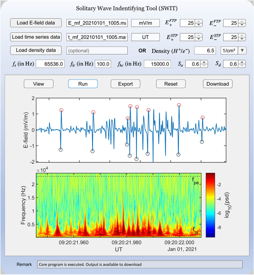
Figure 5. GUI of SWIT, featuring multiple buttons, input fields, and two subplots for waveform visualization. In the waveform panel, the red and blue circles indicate the $E_{+}$ and $E_{-}$ of identified solitary wave structures in a burst dataset by SWIT. The horizontal black dashed lines in the spectrogram indicate electron and ion plasma frequencies.

Other parameters like $S_a$ and $S_d$ that show amplitude and width symmetry are set to 0.6 (recommended limit). Users can vary it between 0.6-1, where 1 represents 100% symmetry and width match, which is an ideal scenario. The threshold values for $E_{\pm }^{\mathit{FTP}}$ and $E_{\pm }^{\mathit{STP}}$ are set to 25% which are recommended limits. Users can reduce these numbers to zero, which means there are no oscillations attached to solitary wave, which depicts an ideal case.

Once the electric field data is loaded, the user can click on the “View” button to plot the electric field in the upper panel and its spectrogram in the lower panel. There will be two horizontal black dashed lines in the lower panel corresponding to the electron plasma frequency $(f_{pe})$ and ion plasma frequency $(f_{pi})$. This will provide a hint to the user as to whether the solitary waves are driven by electrons or ions. Solitary waves are often associated with an enhancement in the power spectral density (PSD) across a broad frequency range. If the enhanced frequencies lie below the ion plasma frequency, the waves are likely to be ion-driven. Conversely, if the frequencies fall between the ion and electron plasma frequencies, the waves are likely to be driven by electrons. Next, by clicking the “Run” button, the user can execute the internal program to identify solitary waves. It marks $E_{+}$ and $E_{-}$ with red and blue circles, respectively, in the upper panel. The plotted Figure can be exported in various formats, such as $.fig$, $.jpeg$, $.png$, $.eps$, $.tif$, and $.pdf$. A “Download” button allows users to save the output in $.mat$, $.dat$, $.txt$, $.csv$, and $.xlsx$ file formats. The output file consists of a matrix with six columns, where the number of rows equals the number of solitary waves identified. These columns, respectively, indicate the $E_{+}$, $E_{-}$, $t_{+}$, $t_{-}$, solitary wave width, and type (either 1 or 2) for identified solitary waves. To reuse the program, the user can click the “Reset” button. The error message or running status of the program is displayed in the remark field provided at the bottom side of the GUI window.

To evaluate SWIT’s baseline performance, we used a Dell G15 5,330 system with Windows 11, powered by 13th-generation Intel Core i5-13450HX CPU (2.4 GHz), and 16 GB RAM. The start-up time of SWIT is approximately 6–9 s after launch. Its RAM usage, measured as the active private working set, ranges from 100 to 300 MB. The total memory footprint (working set) is approximately 900 MB, including around 200 MB of shared memory. We evaluated the CPU time required for data loading and visualization. For example, loading a 62.5 ms signal sampled at 65,536 Hz takes approximately 0.6 ms. On average, loading a 1-s burst signal takes around 8 ms. Similarly, the time required to plot the signal and its spectrogram also varies with signal length. For a 1-s signal, rendering both panels takes about 3 s of CPU time.

5 Results

In this section, we discuss the efficiency of SWIT and some results based on the analysis of medium-frequency calibrated burst mode electric field data from MAVEN for February 2015. In the development of SWIT, we ensure high efficiency, which is needed for the automatic identifier. However, in spite of all these measures, the automatic program may detect some solitary waves, which may be either false positive or false negative. Therefore, the number of solitary waves identified by visual inspection and through automatic programs can differ. In such a scenario, one needs to check the efficiency of SWIT by comparing the number of solitary waves identified visually and through SWIT. For this purpose, we took the electric field data from 1 January 2021 as an example. It contains 2,966 individual burst datasets having durations between 62.5 and 375 ms. Each individual burst is loaded in SWIT GUI with recommended input criteria (i.e., $S_a$ = 0.6, $S_d$ = 0.6, $E_{\pm }^{\mathit{FTP}}$ = 25%, and $E_{\pm }^{\mathit{STP}}$ = 25%), and solitary wave characteristics are documented. Next, for all these individual 2,966 bursts, through visual inspection, we identified the presence or absence of solitary waves and noted the total number of solitary waves for each bursts. This analysis is summarized in the Appendix Table A1. Figure 6 represents the four different burst signals from panel (A)-(D) observed on 1 January 2021. Panels (A) and (B) represent good examples of burst illustrating a series of solitary waves. Whereas panels (C) and (D) of Figure 6 represent burst examples with no solitary waves. It may be noted that in panel (A), there is one solitary wave, which is marked with a dashed rectangle. This solitary wave was selected in visual inspection, but SWIT discarded it. This is the case of a false negative. This solitary wave was discarded by SWIT due to the presence of more than one turning point in $E^{\prime }(t)$ between $t_{-}$ and $t_{+}$ as described in Section 3.2. However, SWIT has identified major solitary wave structures. In Figure 7A, we have plotted the number of solitary waves identified by SWIT (red circle) and through visual inspection (blue asterisk) for bursts grouped in 10 bins. Here, each bin contains 296 burst datasets, except for the last one, which contains 302. The corresponding efficiency is shown in Figure 7B. One can see that for most of the bins, efficiency is above 90%. Overall, a total of 738 solitary waves have been identified by visual inspection, whereas SWIT identifies 698 solitary waves. This clearly indicates that SWIT operates with high efficiency. We defined efficiency as, $ϵ=1-[|N_{\mathit{obs}}-N_{\mathit{SWIT}}|/max\{N_{\mathit{obs}},N_{\mathit{SWIT}}\}]$. The efficiency, $ϵ$ can vary between 0–1, where 1 indicates 100% efficiency. For 1 January 2021, the average efficiency is $⟨ϵ⟩=$ 0.94.

Figure 6

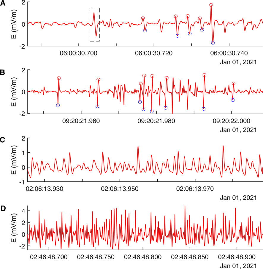
Figure 6. Four examples of electric field burst datasets: (A) A good case where solitary waves have been identified with one false negative solitary wave waveform (see solitary wave marked with a dashed rectangle). (B) Shows another case where all solitary waves have correctly identified. (C,D) Depict cases with no solitary waves, and SWIT GUI does not detect solitary waves for these two cases.

Figure 7

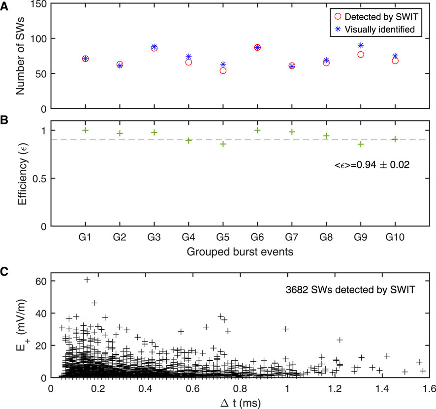
Figure 7. (A) Represents the number of solitary waves detected visually and by SWIT for 2,966 burst events on 1 January 2021. These events are grouped in 10 bins, and the total number of solitary waves in each bin is plotted. Solitary waves identified by SWIT are marked with red circles, while those identified visually are shown with blue asterisks. The corresponding efficiency of SWIT is shown in (B). The dashed line in (B) indicates the 90% efficiency. The mass plot of the peak electric field amplitude as a function of the width of solitary wave identified by SWIT by processing 50,835 burst events recorded on 19 days in February 2015 is shown in (C).

To justify the choice of parameters $S_a$, $S_d$, and the turning points threshold, we considered $S_a$ and $S_d$ values of 0.55, 0.60, and 0.65, and turning points thresholds of 22.5%, 25.0%, and 27.5%. (see Table 1). Efficiency was estimated by comparing solitary waves identified through (i) visual inspection and (ii) SWIT. This analysis was performed for burst events on 1 January 2021. The efficiency was found to be highest when $S_a$ and $S_d$ were set to 0.60, and the turning points threshold to 25%. A confusion matrix corresponding to these optimal values is provided in the Appendix (see Table A2).

Table 1

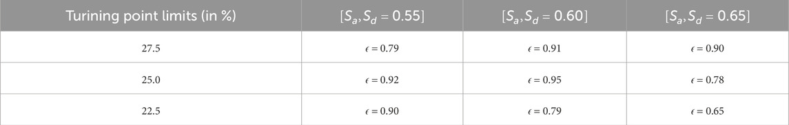
Table 1. The efficiency $(ϵ)$ is evaluated by varying $S_a$ and $S_d$ over the values 0.55, 0.60, and 0.65, and the turning point limits to 22.5%, 25%, and 27.5%. The maximum efficiency is observed when $S_a$ and $S_d$ are both set to 0.60, and the turning point limit is 25%.

Further, to test SWIT, we analyzed the electric field burst datasets for 19 days in February 2015. A total of 50,835 bursts were recorded during February 2015. SWIT identified a total of 3,682 solitary waves. The mean amplitude and width of these waves are approximately 3.2 mV/m and 0.328 ms, respectively (see Table A3). The amplitude as a function of width is shown in Figure 7C for these identified solitary waves. It may be noted that, in general, the amplitude varies between $\sim 0.5-60$ mV/m, and the durations vary between $\sim 0.5-1.5$ ms for the considered datasets. The number of solitary waves identified in a given signal through visual inspection can vary with individual users. This variability arises because many solitary waves observed may deviate from their ideal form (refer to Figure 1). While building a SWIT, we have defined a series of criteria for identifying solitary waves. If any criterion is nearly satisfied but not fully met, the program rejects the waveform to identify it as a solitary wave. For instance, we impose a condition requiring up to 40% deviation between $E_{\mathit{max}}$ and $E_{\mathit{min}}$. If the symmetry is 59.9%, the program will reject the solitary wave waveform. However, a user may not visually recognize the difference between 60% and 59.9% deviation. This scenario can slightly affect the detection of solitary waves. Nonetheless, these criteria are essential to minimize the identification of false positives. Sometimes, a solitary wave is embedded within random oscillations. While such a solitary wave may not be considered significant during visual inspection, SWIT can identify it if all the defined conditions are met.

6 Summary and conclusion

The paper presents a new automatic tool to identify bipolar solitary waves from high-resolution electric field measurements by a spacecraft. It is named as SWIT and is well tested for the medium-frequency (100 Hz–32 kHz) calibrated burst mode electric field data recorded by MAVEN spacecraft. We began by discussing features of the ideal form of the solitary waves and then compared them with the observed electric field bipolar pulse. Accordingly, the criteria to identify solitary waves in the electric field data were built. The series of implemented criteria and their significance in the logical development of the computer program are elaborated. Fundamentally, SWIT is based on the cumulative integration of filtered electric field signals to identify the locations of the bipolar structures present in the data. In the output, SWIT provide $E_{+}$ and $E_{-}$ of solitary waves, with their time of occurrence $t_{+}$ and $t_{-}$, type (i.e., type-1 or type-2) and width (in milliseconds). Additionally, the Figure visible in GUI can be exported in $.fig$, $.jpeg$, $.png$, $.eps$, $.tif$, and $.pdf$ formats. SWIT is optimized for scalability with medium-frequency burst mode electric field data. The burst durations are in multiples of 62.5 ms and could go up to 437.5 ms. The efficiency of SWIT is tested with the medium frequency electric field data recorded by MAVEN, which is found to be above 90%. While SWIT effectively identifies bipolar solitary waves, their interpretation as phase space holes or acoustic solitons is beyond the scope of the present work. Additionally, it should be noted that MAVEN measures only a single component of the electric field, which can limit the detection of solitary waves depending on the angle between the wave propagation direction and the orientation of the probes, i.e., the y-axis of the spacecraft coordinate system.

The SWIT GUI is developed using MATLAB 2024b as a stand-alone desktop application for Windows. In order to run this application, users need the MATLAB Runtime, which is included in the installer. The instructions for the installation and usage of SWIT can be found in the accompanying ReadMe file. Initially, using “process_burst_events.m” program file for MATLAB, the user can convert electric field raw data into individual “.mat” files that contain the electric field and time information separately for each burst files that occurred on a given day. These individual burst files (time and electric field) serve as input to the SWIT module. The recommended parameters for $S_a$, $S_d$, $E_{\pm }^{\mathit{FTP}}$ and $E_{\pm }^{\mathit{STP}}$ are 0.6, 0.6, 25% and 25%, respectively. However, the user can change these parameters. When $S_a$ and $S_d$ are increased and/or $E_{\pm }^{\mathit{FTP}}$ and $E_{\pm }^{\mathit{STP}}$ are decreased, then the conditions tend towards the ideal solitary wave.

SWIT serves as an important resource for conducting detailed statistical analyses, enabling users to explore the characteristics of solitary waves and their relationships with altitude, local time, and space weather conditions, particularly for the Martian plasma environment. The insights gained from this analysis help in understanding the generation of solitary waves in the plasma environment of unmagnetized planets like Mars. This automatic tool will reduce analysis time and aid in processing large-scale, high-resolution data acquired by spacecraft. SWIT is a versatile package that allows modifications in its code to make it applicable for high-resolution electric field datasets from other spacecraft, enabling comparative studies of solitary waves across different planetary plasma environments. In a nutshell, SWIT will be useful to explore the dynamics of bipolar solitary wave structures with good accuracy and efficiency in planetary plasma environments.

Data availability statement

The original contributions presented in the study are included in the article/supplementary material, further inquiries can be directed to the corresponding author.

Author contributions

SP: Methodology, Validation, Investigation, Writing – review and editing, Writing – original draft, Formal Analysis, Visualization, Software. AK: Methodology, Conceptualization, Supervision, Investigation, Funding acquisition, Writing – review and editing, Project administration, Visualization, Software. BK: Visualization, Validation, Investigation, Conceptualization, Writing – review and editing, Supervision, Methodology, Software.

Funding

The author(s) declare that financial support was received for the research and/or publication of this article. Authors acknowledge support from the Indian Institute of Geomagnetism (IIG) India for research funding under the project IIG/MI-PEARL/2024–2025.

Acknowledgments

We thank the MAVEN team for making this valuable data available to the scientific community. This work is supported by the Indian Institute of Geomagnetism under the program MI-PEARL/2024-2025.

Conflict of interest

The authors declare that the research was conducted in the absence of any commercial or financial relationships that could be construed as a potential conflict of interest.

Generative AI statement

The author(s) declare that no Generative AI was used in the creation of this manuscript.

Any alternative text (alt text) provided alongside figures in this article has been generated by Frontiers with the support of artificial intelligence and reasonable efforts have been made to ensure accuracy, including review by the authors wherever possible. If you identify any issues, please contact us.

Publisher’s note

All claims expressed in this article are solely those of the authors and do not necessarily represent those of their affiliated organizations, or those of the publisher, the editors and the reviewers. Any product that may be evaluated in this article, or claim that may be made by its manufacturer, is not guaranteed or endorsed by the publisher.

References

Andersson, L. (2024). MAVEN LPW medium frequency burst mode calibrated electric-field data collection. doi:10.17189/8DBB-Y985

CrossRef Full Text | Google Scholar

Andersson, L., and Ergun, R. E. (2012). “The search for double layers in space plasmas,”, 197. Washington, DC: American Geophysical Union, 241–250. doi:10.1029/2011GM001170

CrossRef Full Text | Google Scholar

Andersson, L., Ergun, R., Delory, G., Eriksson, A., Westfall, J., Reed, H., et al. (2015). The langmuir probe and waves (LPW) instrument for MAVEN. Space Sci. Rev. 195, 173–198. doi:10.1007/s11214-015-0194-3

CrossRef Full Text | Google Scholar

Aravindakshan, H., Kakad, A., and Kakad, B. (2018a). Bernstein-greene-kruskal theory of electron holes in superthermal space plasma. Phys. Plasmas 25, 052901. doi:10.1063/1.5025234

CrossRef Full Text | Google Scholar

Aravindakshan, H., Kakad, A., and Kakad, B. (2018b). Effects of wave potential on electron holes in thermal and superthermal space plasmas. Phys. Plasmas 25, 122901. doi:10.1063/1.5046721

CrossRef Full Text | Google Scholar

Aravindakshan, H., Yoon, P. H., Kakad, A., and Kakad, B. (2020). Theory of ion holes in space and astrophysical plasmas. Mon. Notices R. Astronomical Soc. Lett. 497, L69–L75. doi:10.1093/mnrasl/slaa114

CrossRef Full Text | Google Scholar

Aravindakshan, H., Kakad, A., Kakad, B., and Yoon, P. H. (2021). Structural characteristics of ion holes in plasma. Plasma 4, 435–449. doi:10.3390/plasma4030032

CrossRef Full Text | Google Scholar

Aravindakshan, H., Vasko, I. Y., Kakad, A., Kakad, B., and Wang, R. (2023). Theory of ion holes in plasmas with flat-topped electron distributions. Phys. Plasmas 30, 022903. doi:10.1063/5.0086613

CrossRef Full Text | Google Scholar

Arya, N., and Kakad, A. (2025). Lower hybrid and solitary waves in dusk flank region of the earth’s magnetosphere. Adv. Space Res. 75, 876–885. doi:10.1016/j.asr.2024.08.065

CrossRef Full Text | Google Scholar

Cattell, C., Crumley, J., Dombeck, J., Wygant, J., and Mozer, F. (2002). Polar observations of solitary waves at the Earth’s magnetopause. Geophys. Res. Lett. 29, 1065. doi:10.1029/2001GL014046

CrossRef Full Text | Google Scholar

Dillard, C., Vasko, I., Mozer, F., Agapitov, O., and Bonnell, J. (2018). Electron-acoustic solitary waves in the Earth’s inner magnetosphere. Phys. Plasmas 25, 022905. doi:10.1063/1.5007907

CrossRef Full Text | Google Scholar

Eliasson, B., and Shukla, P. K. (2006). Formation and dynamics of coherent structures involving phase-space vortices in plasmas. Phys. Rep. 422, 225–290. doi:10.1016/j.physrep.2005.10.003

CrossRef Full Text | Google Scholar

Ergun, R., Carlson, C., McFadden, J., Mozer, F., Muschietti, L., Roth, I., et al. (1998). Debye-scale plasma structures associated with magnetic-field-aligned electric fields. Phys. Rev. Lett. 81, 826–829. doi:10.1103/PhysRevLett.81.826

CrossRef Full Text | Google Scholar

Ergun, R., Andersson, L., Main, D., Su, Y.-J., Newman, D., Goldman, M., et al. (2004). Auroral particle acceleration by strong double layers: the upward current region. J. Geophys. Res. Space Phys. 109, A12220. doi:10.1029/2004JA010545

CrossRef Full Text | Google Scholar

Ergun, R., Andersson, L., Tao, J., Angelopoulos, V., Bonnell, J., McFadden, J., et al. (2009). Observations of double layers in Earth’s plasma sheet. Phys. Rev. Lett. 102, 155002. doi:10.1103/PhysRevLett.102.155002

PubMed Abstract | CrossRef Full Text | Google Scholar

Graham, D. B., Khotyaintsev, Y. V., Vaivads, A., and André, M. (2015). Electrostatic solitary waves with distinct speeds associated with asymmetric reconnection. Geophys. Res. Lett. 42, 215–224. doi:10.1002/2014GL062538

CrossRef Full Text | Google Scholar

Graham, D. B., Khotyaintsev, Y. V., Vaivads, A., and Andre, M. (2016). Electrostatic solitary waves and electrostatic waves at the magnetopause. J. Geophys. Res. Space Phys. 121, 3069–3092. doi:10.1002/2015JA021527

CrossRef Full Text | Google Scholar

Hansel, P. J., Wilder, F., Malaspina, D. M., Ergun, R. E., Ahmadi, N., Holmes, J. C., et al. (2021). Mapping MMS observations of solitary waves in Earth’s magnetic field. J. Geophys. Res. Space Phys. 126, e2021JA029389. doi:10.1029/2021JA029389

CrossRef Full Text | Google Scholar

Hobara, Y., Walker, S., Balikhin, M., Pokhotelov, O., Gedalin, M., Krasnoselskikh, V., et al. (2008). Cluster observations of electrostatic solitary waves near the earth’s bow shock. J. Geophys. Res. Space Phys. 113, A05211. doi:10.1029/2007JA012789

CrossRef Full Text | Google Scholar

Holmes, J., Ergun, R., Newman, D., Wilder, F., Sturner, A., Goodrich, K., et al. (2018). Negative potential solitary structures in the magnetosheath with large parallel width. J. Geophys. Res. Space Phys. 123, 132–145. doi:10.1002/2017JA024890

CrossRef Full Text | Google Scholar

Kakad, A., and Kakad, B. (2019). Generation of series of electron Acoustic solitary wave pulses in plasma. Phys. Plasmas 26, 102105. doi:10.1063/1.5113743

CrossRef Full Text | Google Scholar

Kakad, A., Singh, S., Reddy, R., Lakhina, G., Tagare, S., and Verheest, F. (2007). Generation mechanism for electron acoustic solitary waves. Phys. plasmas 14, 052305. doi:10.1063/1.2732176

CrossRef Full Text | Google Scholar

Kakad, A., Singh, S., Reddy, R., Lakhina, G., and Tagare, S. (2009). Electron acoustic solitary waves in the Earth’s magnetotail region. Adv. Space Res. 43, 1945–1949. doi:10.1016/j.asr.2009.03.005

CrossRef Full Text | Google Scholar

Kakad, A., Omura, Y., and Kakad, B. (2013). Experimental evidence of ion acoustic soliton chain formation and validation of nonlinear fluid theory. Phys. Plasmas 20, 062103. doi:10.1063/1.4810794

CrossRef Full Text | Google Scholar

Kakad, B., Kakad, A., and Omura, Y. (2014). Nonlinear evolution of ion acoustic solitary waves in space plasmas: fluid and particle-in-cell simulations. J. Geophys. Res. Space Phys. 119, 5589–5599. doi:10.1002/2014JA019798

CrossRef Full Text | Google Scholar

Kakad, A., Kakad, B., Anekallu, C., Lakhina, G., Omura, Y., and Fazakerley, A. (2016). Slow electrostatic solitary waves in Earth’s plasma sheet boundary layer. J. Geophys. Res. Space Phys. 121, 4452–4465. doi:10.1002/2016JA022365

CrossRef Full Text | Google Scholar

Kakad, A., Kakad, B., and Omura, Y. (2017a). Formation and interaction of multiple coherent phase space structures in plasma. Phys. Plasmas 24, 060704. doi:10.1063/1.4986109

CrossRef Full Text | Google Scholar

Kakad, B., Kakad, A., and Omura, Y. (2017b). Particle trapping and ponderomotive processes during breaking of ion acoustic waves in plasmas. Phys. Plasmas 24, 102122. doi:10.1063/1.4986030

CrossRef Full Text | Google Scholar

Kakad, B., Kakad, A., Aravindakshan, H., and Kourakis, I. (2022). Debye-scale solitary structures in the Martian magnetosheath. Astrophysical J. 934, 126. doi:10.3847/1538-4357/ac7b8b

CrossRef Full Text | Google Scholar

Kamaletdinov, S., Vasko, I., Wang, R., Artemyev, A., Yushkov, E., and Mozer, F. (2022). Slow electron holes in the Earth’s bow shock. Phys. Plasmas 29, 092303. doi:10.1063/5.0102289

CrossRef Full Text | Google Scholar

Kojima, H., Omura, Y., Matsumoto, H., Miyaguti, K., and Mukai, T. (2000). Automatic waveform selection method for electrostatic solitary waves. Earth, planets space 52, 495–502. doi:10.1186/BF03351653

CrossRef Full Text | Google Scholar

Krasovsky, V., Matsumoto, H., and Omura, Y. (1997). Bernstein-greene-kruskal analysis of electrostatic solitary waves observed with geotail. J. Geophys. Res. Space Phys. 102, 22131–22139. doi:10.1029/97JA02033

CrossRef Full Text | Google Scholar

Lakhina, G., Kakad, A., Singh, S., and Verheest, F. (2008a). Ion-and electron-acoustic solitons in two-electron temperature space plasmas. Phys. Plasmas 15, 062903. doi:10.1063/1.2930469

CrossRef Full Text | Google Scholar

Lakhina, G., Singh, S., Kakad, A., Verheest, F., and Bharuthram, R. (2008b). Study of nonlinear ion-and electron-acoustic waves in multi-component space plasmas. Nonlinear Process. Geophys. 15, 903–913. doi:10.5194/npg-15-903-2008

CrossRef Full Text | Google Scholar

Lakhina, G., Singh, S., Kakad, A., Goldstein, M., Vinas, A., and Pickett, J. (2009). A mechanism for electrostatic solitary structures in the Earth’s magnetosheath. J. Geophys. Res. Space Phys. 114, A09212. doi:10.1029/2009JA014306

CrossRef Full Text | Google Scholar

Lakhina, G., Singh, S., Kakad, A., and Pickett, J. (2011a). Generation of electrostatic solitary waves in the plasma sheet boundary layer. J. Geophys. Res. Space Phys. 116. doi:10.1029/2011JA016700

CrossRef Full Text | Google Scholar

Lakhina, G. S., Singh, S., and Kakad, A. (2011b). Ion-and electron-acoustic solitons and double layers in multi-component space plasmas. Adv. Space Res. 47, 1558–1567. doi:10.1016/j.asr.2010.12.013

CrossRef Full Text | Google Scholar

Lakhina, G. S., Singh, S., Rubia, R., and Devanandhan, S. (2021). Electrostatic solitary structures in space plasmas: Soliton perspective. Plasma 4, 681–731. doi:10.3390/plasma4040035

CrossRef Full Text | Google Scholar

Lotekar, A., Kakad, A., and Kakad, B. (2016). Fluid simulation of dispersive and nondispersive ion acoustic waves in the presence of superthermal electrons. Phys. Plasmas 23, 102108. doi:10.1063/1.4964478

CrossRef Full Text | Google Scholar

Lotekar, A., Kakad, A., and Kakad, B. (2017). Generation of ion acoustic solitary waves through wave breaking in superthermal plasmas. Phys. Plasmas 24, 102127. doi:10.1063/1.4991467

CrossRef Full Text | Google Scholar

Lotekar, A., Kakad, A., and Kakad, B. (2019). Formation of asymmetric electron acoustic double layers in the Earth’s inner magnetosphere. J. Geophys. Res. Space Phys. 124, 6896–6905. doi:10.1029/2018JA026303

CrossRef Full Text | Google Scholar

Maharaj, S., Bharuthram, R., Singh, S., and Lakhina, G. (2015). Existence domains of slow and fast ion-acoustic solitons in two-ion space plasmas. Phys. Plasmas 22, 032313. doi:10.1063/1.4916319

CrossRef Full Text | Google Scholar

Malaspina, D. M., Goodrich, K., Livi, R., Halekas, J., McManus, M., Curry, S., et al. (2020). Plasma double layers at the boundary between Venus and the solar wind. Geophys. Res. Lett. 47, e2020GL090115. doi:10.1029/2020GL090115

PubMed Abstract | CrossRef Full Text | Google Scholar

Matsumoto, H., Kojima, H., Miyatake, T., Omura, Y., Okada, M., Nagano, I., et al. (1994). Electrostatic solitary waves (ESW) in the magnetotail: BEN wave forms observed by GEOTAIL. Geophys. Res. Lett. 21, 2915–2918. doi:10.1029/94gl01284

CrossRef Full Text | Google Scholar

Mozer, F., Bale, S., Bonnell, J., Chaston, C., Roth, I., and Wygant, J. (2013). Megavolt parallel potentials arising from double-layer streams in the earth’s outer radiation belt. Phys. Rev. Lett. 111, 235002. doi:10.1103/PhysRevLett.111.235002

PubMed Abstract | CrossRef Full Text | Google Scholar

Mozer, F., Agapitov, O., Giles, B., and Vasko, I. (2018). Direct observation of electron distributions inside millisecond duration electron holes. Phys. Rev. Lett. 121, 135102. doi:10.1103/PhysRevLett.121.135102

PubMed Abstract | CrossRef Full Text | Google Scholar

Norgren, C., André, M., Vaivads, A., and Khotyaintsev, Y. V. (2015). Slow electron phase space holes: Magnetotail observations. Geophys. Res. Lett. 42, 1654–1661. doi:10.1002/2015GL063218

CrossRef Full Text | Google Scholar

Olivier, C., Maharaj, S., and Bharuthram, R. (2015). Ion-acoustic solitons, double layers and supersolitons in a plasma with two ion-and two electron species. Phys. Plasmas 22, 082312. doi:10.1063/1.4928884

CrossRef Full Text | Google Scholar

Omura, Y., Matsumoto, H., Miyake, T., and Kojima, H. (1996). Electron beam instabilities as generation mechanism of electrostatic solitary waves in the magnetotail. J. Geophys. Res. Space Phys. 101, 2685–2697. doi:10.1029/95JA03145

CrossRef Full Text | Google Scholar

Pandey, S., Kakad, A., and Kakad, B. (2025a). First observational evidence of plasma waves in the Martian magnetosheath jet. Mon. Notices R. Astronomical Soc. Lett. 537, L7–L13. doi:10.1093/mnrasl/slae105

CrossRef Full Text | Google Scholar

Pandey, S., Kakad, A., and Kakad, B. (2025b). Solitary wave identifying tool (SWIT) for electric field dataset from MAVEN spacecraft. doi:10.5281/zenodo.15174978

CrossRef Full Text | Google Scholar

Pandey, S., Kakad, A., Kakad, B., Singh, K., and Kourakis, I. (2025c). Double layers in the Martian magnetosheath. Astrophysical J. 981, 44. doi:10.3847/1538-4357/adad6f

CrossRef Full Text | Google Scholar

Pickett, J., Menietti, J., Gurnett, D., Tsurutani, B., Kintner, P., Klatt, E., et al. (2003). Solitary potential structures observed in the magnetosheath by the cluster spacecraft. Nonlinear Process. Geophys. 10, 3–11. doi:10.5194/npg-10-3-2003

CrossRef Full Text | Google Scholar

Pickett, J., Kahler, S., Chen, L.-J., Huff, R., Santolik, O., Khotyaintsev, Y., et al. (2004). Solitary waves observed in the auroral zone: the cluster multi-spacecraft perspective. Nonlinear Process. Geophys. 11, 183–196. doi:10.5194/npg-11-183-2004

CrossRef Full Text | Google Scholar

Pickett, J., Chen, L.-J., Kahler, S., Santolik, O., Goldstein, M., Lavraud, B., et al. (2005). On the generation of solitary waves observed by cluster in the near-Earth magnetosheath. Nonlinear Process. Geophys. 12, 181–193. doi:10.5194/npg-12-181-2005

CrossRef Full Text | Google Scholar

Rubia, R., Singh, S., Lakhina, G., Devanandhan, S., Dhanya, M., and Kamalam, T. (2023). Electrostatic solitary waves in the venusian ionosphere pervaded by the solar wind: a theoretical perspective. Astrophysical J. 950, 111. doi:10.3847/1538-4357/acd2d7

CrossRef Full Text | Google Scholar

Shaikh, Z., Vasko, I., Hutchinson, I., Kamaletdinov, S., Holmes, J., Newman, D., et al. (2024). Slow electron holes in the Earth’s magnetosheath. J. Geophys. Res. Space Phys. 129, e2023JA032059. doi:10.1029/2023JA032059

CrossRef Full Text | Google Scholar

Singh, S., and Lakhina, G. (2001). Generation of electron-acoustic waves in the magnetosphere. Planet. Space Sci. 49, 107–114. doi:10.1016/S0032-0633(00)00126-4

CrossRef Full Text | Google Scholar

Singh, K., Kakad, A., Kakad, B., and Kourakis, I. (2022). Fluid simulation of dust-acoustic solitary waves in the presence of suprathermal particles: application to the magnetosphere of Saturn. Astronomy and Astrophysics 666, A37. doi:10.1051/0004-6361/202244136

CrossRef Full Text | Google Scholar

Singh, K., Varghese, S. S., Saini, N. S., and Kourakis, I. (2024). Oblique electrostatic solitary and supersolitary waves in earth’s magnetosheath. Astrophysical J. 971, 25. doi:10.3847/1538-4357/ad5c6b

CrossRef Full Text | Google Scholar

Sun, J., Vasko, I. Y., Bale, S. D., Wang, R., and Mozer, F. S. (2022). Double layers in the Earth’s bow shock. Geophys. Res. Lett. 49, e2022GL101348. doi:10.1029/2022GL101348

CrossRef Full Text | Google Scholar

Temerin, M., Cerny, K., Lotko, W., and Mozer, F. (1982). Observations of double layers and solitary waves in the auroral plasma. Phys. Rev. Lett. 48, 1175–1179. doi:10.1103/PhysRevLett.48.1175

CrossRef Full Text | Google Scholar

Thaller, S. A., Andersson, L., Schwartz, S. J., Mazelle, C., Fowler, C., Goodrich, K., et al. (2022). Bipolar electric field pulses in the Martian magnetosheath and solar wind; their implication and impact accessed by system scale size. J. Geophys. Res. Space Phys. 127, e2022JA030374. doi:10.1029/2022JA030374

PubMed Abstract | CrossRef Full Text | Google Scholar

Tong, Y., Vasko, I., Mozer, F., Bale, S. D., Roth, I., Artemyev, A., et al. (2018). Simultaneous multispacecraft probing of electron phase space holes. Geophys. Res. Lett. 45, 11–513. doi:10.1029/2018GL079044

CrossRef Full Text | Google Scholar

Umeda, T., Omura, Y., Matsumoto, H., and Usui, H. (2002). Formation of electrostatic solitary waves in space plasmas: particle simulations with open boundary conditions. J. Geophys. Res. Space Phys. 107, 1449. doi:10.1029/2001JA000286

CrossRef Full Text | Google Scholar

Varghese, S. S., Singh, K., and Kourakis, I. (2024a). Electrostatic solitary waves in a bi-ion plasma with two suprathermal electron populations–application to Saturn’s magnetosphere. Mon. Notices R. Astronomical Soc. 527, 8337–8354. doi:10.1093/mnras/stad3763

CrossRef Full Text | Google Scholar

Varghese, S. S., Singh, K., Verheest, F., and Kourakis, I. (2024b). Electrostatic solitary waves in electronegative Martian plasma. Astrophysical J. 977, 100. doi:10.3847/1538-4357/ad8b49

CrossRef Full Text | Google Scholar

Vasko, I., Agapitov, O., Mozer, F., Bonnell, J., Artemyev, A., Krasnoselskikh, V., et al. (2017a). Electron-acoustic solitons and double layers in the inner magnetosphere. Geophys. Res. Lett. 44, 4575–4583. doi:10.1002/2017gl074026

CrossRef Full Text | Google Scholar

Vasko, I., Kuzichev, I., Agapitov, O., Mozer, F., Artemyev, A., and Roth, I. (2017b). Evolution of electron phase space holes in inhomogeneous plasmas. Phys. Plasmas 24, 062311. doi:10.1063/1.4989717

CrossRef Full Text | Google Scholar

Vasko, I., Mozer, F., Krasnoselskikh, V., Artemyev, A., Agapitov, O., Bale, S., et al. (2018). Solitary waves across supercritical quasi-perpendicular shocks. Geophys. Res. Lett. 45, 5809–5817. doi:10.1029/2018GL077835

CrossRef Full Text | Google Scholar

Vasko, I. Y., Wang, R., Mozer, F. S., Bale, S. D., and Artemyev, A. V. (2020). On the nature and origin of bipolar electrostatic structures in the Earth’s bow shock. Front. Phys. 8, 156. doi:10.3389/fphy.2020.00156

CrossRef Full Text | Google Scholar

Wang, R., Lu, Q., Khotyaintsev, Y. V., Volwerk, M., Du, A., Nakamura, R., et al. (2014). Observation of double layer in the separatrix region during magnetic reconnection. Geophys. Res. Lett. 41, 4851–4858. doi:10.1002/2014GL061157

CrossRef Full Text | Google Scholar

Wang, R., Vasko, I., Artemyev, A., Holley, L., Kamaletdinov, S., Lotekar, A., et al. (2022). Multisatellite observations of ion holes in the Earth’s plasma sheet. Geophys. Res. Lett. 49, e2022GL097919. doi:10.1029/2022GL097919

CrossRef Full Text | Google Scholar

Wang, C., Huang, S., Yuan, Z., Jiang, K., Zhang, J., Dong, Y., et al. (2023). In situ observation of electron acceleration by a double layer in the bow shock. Astrophysical J. 952, 78. doi:10.3847/1538-4357/acdacb

CrossRef Full Text | Google Scholar

Williams, J., Chen, L.-J., Kurth, W., Gurnett, D., and Dougherty, M. (2006). Electrostatic solitary structures observed at Saturn. Geophys. Res. Lett. 33, L06103. doi:10.1029/2005GL024532

CrossRef Full Text | Google Scholar

Appendix A

A1 SWIT output summary: 1 January 2021 datasets

TABLE A1

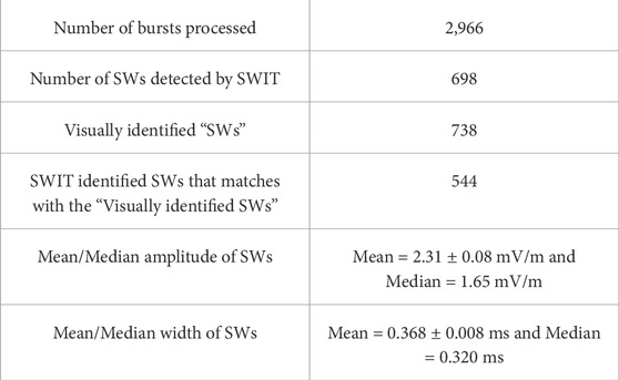
TABLE A1. Summary of SWIT’s output for the dataset from 1 January 2021.

A2 confusion matrix: 1 January 2021 datasets

TABLE A2

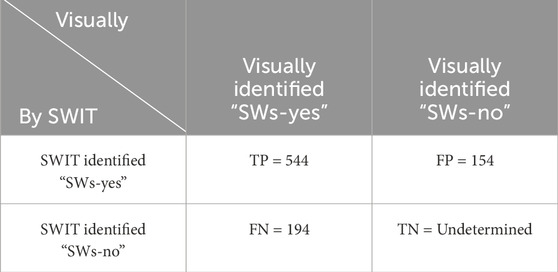
TABLE A2. Confusion matrix based on SWIT’s predictions for the presence of SWs on 1 January 2021. Columns indicate the visually identified presence or absence of SWs, while rows show the SWs detected by SWIT. The False negative rate is estimated to be 0.26.

$\text{False\hspace{0.17em}negative\hspace{0.17em}rate}=\frac{FN}{TP+FN}=\frac{194}{544+194}=0.26$

Our dataset consists of continuous electric field measurements over time, which may include solitary waves (SWs) with varying characteristics (e.g., amplitude and width). Moreover, there is no defined criterion for how many SWs should appear in a given burst signal. The signal segments that exclude visually identified SWs can be considered as true negatives; however, they remain unquantified. Therefore, it is not possible to estimate the number of true negatives.

A3 SWIT output summary: February 2015 datasets

TABLE A3

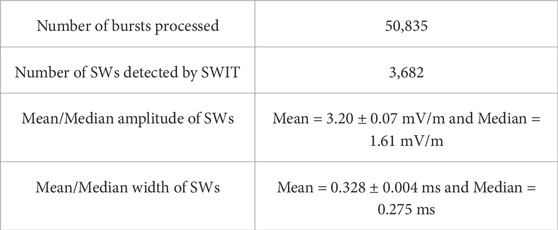
TABLE A3. Summary of SWIT’s output for the dataset from February 2015.