Predictive analytics of cold ion outflow from the Earth’s ionosphere

In this study, we investigate the cold ions ($<$70 eV) originated in the high-latitude ionosphere of the Earth entering the magnetosphere towards the magnetotail. We analyze measurements from Cluster spacecraft along with solar irradiance, solar wind (SW), and geomagnetic observations. Two machine learning models driven by solar irradiance and solar wind measurements are derived to predict the cold ion flux. With the linear baseline model, we provide an empirical formula. The nonlinear model (Extra-Trees Regressor) yields 17% better performance. The total cold ion escape rate from the polar cap ranges between $\sim 1.1\cdot 10^{24}$ and $\sim 2.7\cdot 10^{26}{s}^{-1}$. The upper limit is comparable to the neutral escape rate. The results show that spatial location is the most important predictor. Solar EUV irradiance is also among the top predictors, followed by the solar wind electric field, the interplanetary magnetic field (IMF), and solar wind dynamic pressure. These results can help to evaluate the influence of the stellar wind-magnetospheric interaction on the ion outflow at Earth-like exoplanets. They indicate the importance of such an interaction for the atmospheric escape during active geomagnetic conditions. Stronger outflow from the Northern Hemisphere than from the Southern Hemisphere hints that the magnetic field strength can impact the amount of ionospheric outflow.

1 Introduction

Populations of ions characterized by total energies below 100 eV are termed ‘cold’ (Delzanno et al., 2021). Cold ions within the magnetosphere originate mainly from the ionosphere. The polar cap and the auroral regions are major contributors to ionospheric escape (Kronberg et al., 2014). The variability in the outflow fluxes and composition is strongly influenced by solar and magnetospheric activities (Cully et al., 2003). Under certain conditions, this ionospheric plasma source becomes the predominant plasma contributor within the magnetosphere (Chappell et al., 1987; Welling et al., 2015; Toledo-Redondo et al., 2021). Therefore, ionospheric outflow impacts the dynamics of the magnetosphere and is an important component in understanding geospace dynamics (Kronberg et al., 2021).

Despite their importance, cold populations are amongst the least explored, mainly due to the challenges of obtaining reliable measurements (Delzanno et al., 2021). The challenge is caused by the positive electric charge on the surface of a sunlit spacecraft. Cold ions with kinetic energies lower than the electric potential energy of the spacecraft are not reliably detected by the instruments onboard the spacecraft. Advancements in scientific instrumentation from the Cluster mission (Escoubet et al., 2001) and methodologies from recent research have further expanded the possibilities to quantify the cold plasma population. The Cluster spacecraft have enabled measurements of the cold ion outflow parameters using in situ electric field measurements via the “wake technique” (Pedersen et al., 2008; Engwall et al., 2008; 2009; Lybekk et al., 2012; Li et al., 2012; Li et al., 2013). New insights into this technique are given by André et al. (2021). They also demonstrated observations of boom-induced wake using the MMS mission. A simple linear model for cold ions based on measurements of the Akebono suprathermal mass spectrometer with respect to different solar and geomagnetic parameters was derived by Cully et al. (2003).

In this study, we present linear and ensemble machine learning (ML) models that predict the outflow of cold ions ($<70$ eV) from the polar cap region as a function of solar activity and location parameters. The models can determine important predictors for the cold ion flux and can help to assess the total outflow rate under various activity conditions. The Cluster observations and the technique described in André et al. (2021) are used to obtain the parameters of the cold ions. Quantification and modeling of cold ion outflow help reconstruct total atmospheric escape rates. It puts cold ion outflow in the relative context with neutral particle escape and escape of ions at higher energies, as well as the escape from low and middle latitudes on closed magnetic field lines. This could inform exoplanetary atmospheric modeling studies in evaluating the importance of ionospheric ion outflow.

2 Methods and observations

In the tenuous plasma environment over the polar cap region, a spacecraft can be positively charged due to the photoelectric effect. The spacecraft electric potential, $V_{sc}$, is often a few tens of volts. Its equivalent potential energy is larger than the kinetic energy of cold ionospheric ions (mainly protons), $E_k$. Since the ions are cold, their thermal energy is smaller than their kinetic energy, such that:

$k{T}_i<E_k<e{V}_{sc},(1)$

where $k$ is the Boltzmann constant, $T_i$ is the ion temperature and $e$ is the elementary charge, under the condition in Equation 1, an enhanced plasma wake is formed downstream of the spacecraft. The enhanced wake can be much larger than the size of the spacecraft due to scattering of the cold ions by the positive spacecraft potential. The wake contains almost no cold ions but is filled with cold electrons. The electric field of the wake lies in the same direction as the cold ion flow (Engwall et al., 2006). The wake electric field can be obtained by comparing the data from the Electric Field and Wave (EFW) instrument (Gustafsson et al., 2001) with the data from the Electron Drift Instrument (EDI) (Paschmann et al., 1997). The EFW instrument obtains the electric field between four orthogonally mounted probes on 88-m long wire booms. The EDI infers the electric field by measuring the drift of artificially emitted electrons as they gyrate back to the spacecraft in the geomagnetic field. Considering the geometry relation between the bulk velocity of the cold ion flow and the background magnetic field measured by the fluxgate magnetometer (FGM) (Balogh et al., 2001), the velocities parallel- and perpendicular to the magnetic field components, $v_{\Vert }$ and $v_{\perp }$, can be derived. For more details on this method, we refer to the description in Engwall et al. (2009).

Since $V_{sc}$ is formed due to the balance between the currents of photoelectrons emitting from the spacecraft and the electrons bombarding the spacecraft from background plasma, the density of cold plasma $n_e$ can be derived from $V_{sc}$ as follows:

$n_e=A{e}^{\frac{-V_{sc}}{B}}(2)$

where A and B are depended on spacecraft surface geometry and solar EUV irradiance. They are determined for different years during the solar cycle (Lybekk et al., 2012; Pedersen et al., 2008) and may also be refined for daily solar EUV variations (André et al., 2015). Considering the charge neutrality, the ion density, $n_i$, is identical to the electron density, identified in Equation 2.

Finally, the flux of cold ions along magnetic field lines, $j_i$, is calculated as:

$j_i=n_i{v}_{\Vert i}(3)$

Using the method described above and measurements by Cluster 1 and Cluster 3, André et al. (2015) obtained parameters of the cold ion outflow during the periods between July to November, from 2001–2010, when the satellites remained within the magnetosphere. The measurements by Cluster 2 and Cluster 4 were not used because EDI on those spacecraft were not operated. The measurements during solar minimum of solar cycle 23 (especially in 2008) are not included in the dataset, because solar EUV irradiance was too low, causing the EFW probes operating with a fixed bias current to function improperly. Also measurements of Cluster 3 in 2006 are excluded due to the same reason. Other criteria for the data selection include: 1) reliable EDI measurements, namely, data with missing returning-electron-beam signals and other technical issues were excluded. This led to exclusion of the day side observations as large gradients in the magnetic field prevent the artificially emitted electrons to gyrate back properly to the receiver; the EDI error was incorporated into the total error estimate for cold ion parallel bulk velocity; 2) spacecraft potential within the range from +8 to +50 V, so that the relation in Lybekk et al. (2012) can be used; 3) wake electric field in the range 2–100 mV/m; 4) magnetic field not too perpendicular with respect to the spin plane to ensure reliable calculation of the parallel velocity (Engwall et al., 2009). Uncertainties of the magnetic field measurements are used for the total cold ion bulk velocity error estimation, too; 5) reasonable values of the velocity in the satellite spin plane with small enough relative errors to ensure the detection in the cold ion energy range.

The relative error for ion density $\mathrm{\Delta }(n_i)$ is generally 20%, as given in Lybekk et al. (2012). The relative error for the parallel velocity $\mathrm{\Delta }(v_{\Vert })$ is provided in the dataset from André and Cully (2012). We combine these errors to obtain the total relative error of the flux, defined in Equation 3, as follows:

$\mathrm{\Delta }\left(j_i\right)=\sqrt{\mathrm{\Delta }{\left(n_i\right)}^2+\mathrm{\Delta }{\left(v_{\Vert }\right)}^2}(4)$

We include the total relative errors as input weights in our models, see more details in Section 3.

For more details on this dataset, we refer to the study by André et al. (2015). Values for the aleatoric uncertainty (mean relative error) for the training and test dataset are provided in Table 5. The current dataset contains 320,503 data points with a 4s spacecraft spin resolution. The distribution of the number of flux observations versus flux value and time is shown in Figure 1.

Figure 1

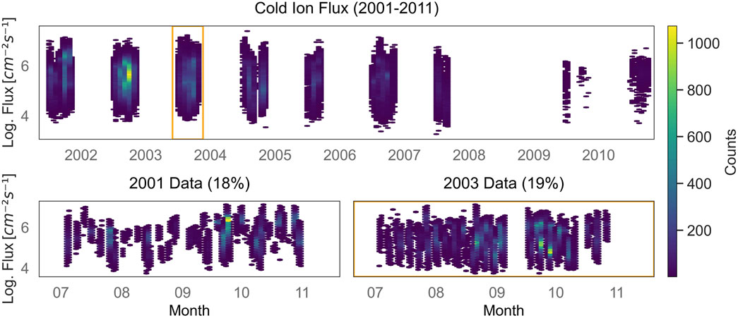
Figure 1. Number of cold ion flux observations versus flux and time for the period from 2001 to 2011 (top). Zoom-ins for 2001 and 2003 show periods selected as best candidates for test data (bottom). The orange rectangle indicates the selected test dataset. See more details about the selection in Section 3.

2.1 Predictors of cold ion flux

Table 1 lists the predictors evaluated for their relevance to model performance. Histograms for the predictors are shown in Figure 2. The numbers of events in the histograms generally represent the full range of parameter values in the dataset, with only a few outliers towards high solar wind and geomagnetic activity.

Table 1

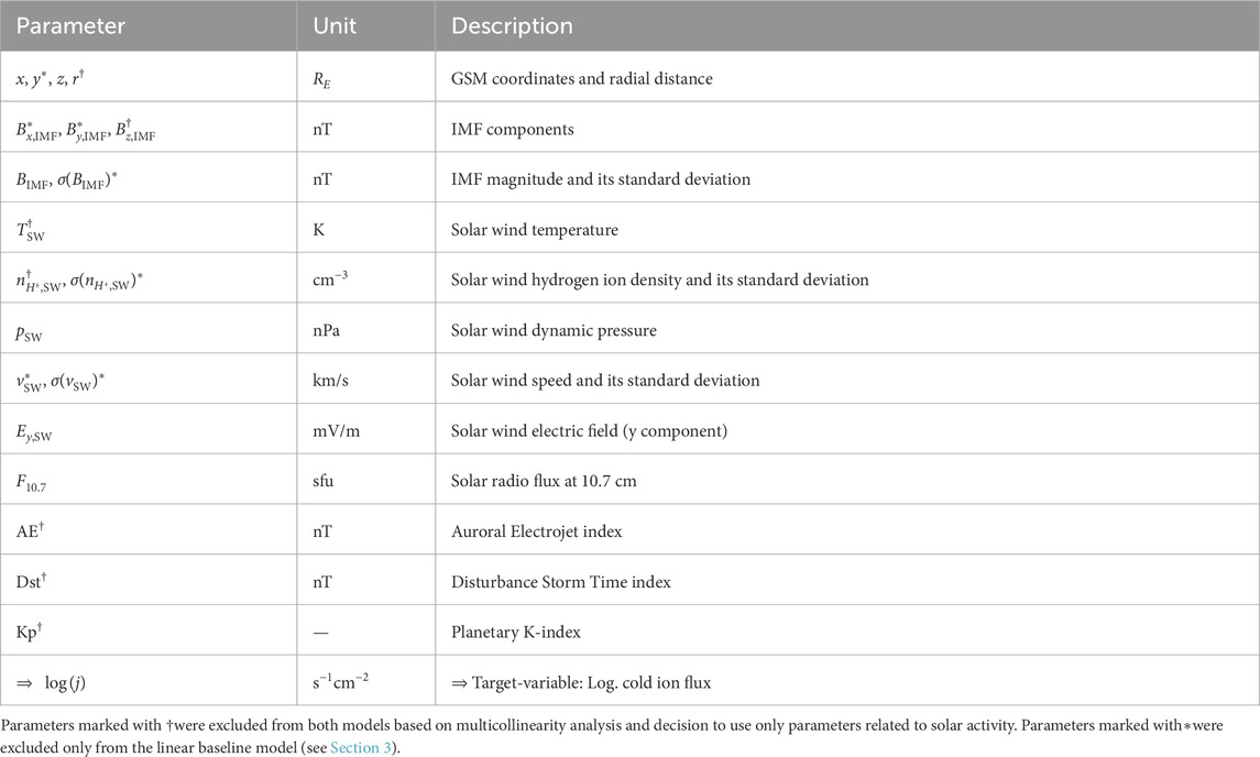
Table 1. Overview of relevant parameters.

Figure 2

Figure 2. Histograms of observed events for different predictor parameters provided in Table 1. Orange vertical lines mark zero values along the x-axis.

2.1.1 Predictors related to location in space

In the presented analysis the flux is systematically correlated with its respective position within the geocentric solar magnetospheric (GSM) coordinate system. The positioning is determined by the spatial parameters $x$, $y$, $z$ and the radial distance from Earth’s center, $r$, expressed in terms of Earth radii, $R_E$. Figure 3 illustrates the spatial distribution of the flux within the GSM coordinates and corresponding spatial data coverage. In Figure 4 logarithmic mean values of the cold ion flux are plotted against the different value ranges of the features. From these plots, we can observe a linear decline of logarithmic cold ion flux with increasing distance for $r$ and $|x|$. This is expected to be due to the diffusion of the ions to a large volume. Higher cold ion flux can be identified in the Northern Hemisphere from Figures 3, 4. Here, we compare regions at $x<\sim$-5 $R_E$, $|y|<\sim$5 $R_E$, and $|z|>\sim$5 $R_E$ where we have a significant amount of observations according to bottom panels of Figure 3. Discussion of the asymmetry can be found in Section 5.

Figure 3

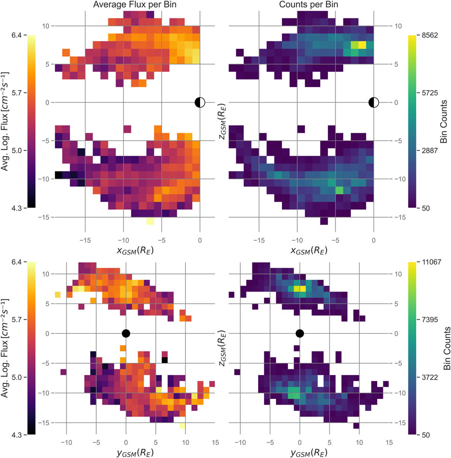
Figure 3. The heatmaps illustrate the spatial distribution of the average logarithmic cold ion flux- (left column) and the counts of data points per bin (right column) in the xz (top) and yz (bottom) GSM planes. The Earth is shown as a circle, where the white half corresponds to the day side and the black half to the night side. Only bins with minimum 20 data points are shown. The bin size is $1R_E\times 1R_E$.

Figure 4

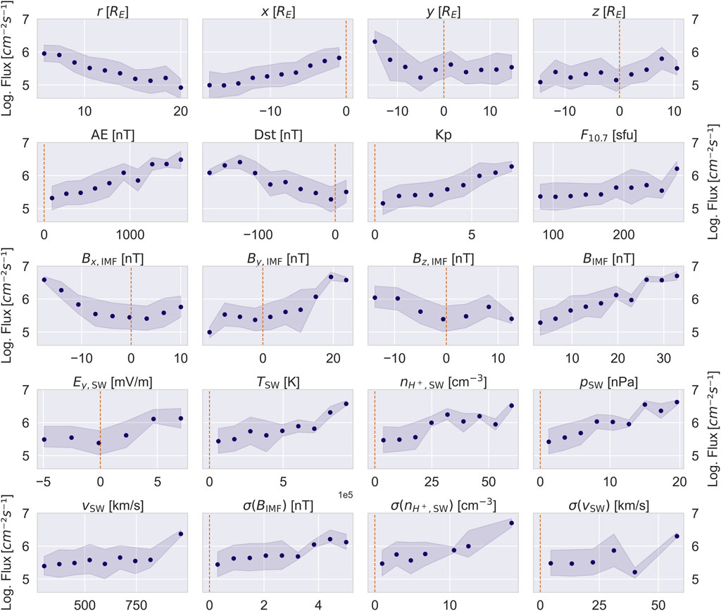
Figure 4. Relationships between the mean cold ion flux and the predictors listed in Table 1. The original range of values for each parameter is divided into 10 bins. The mean flux is computed within each bin, provided that the number of data points in the bin exceeds a minimum threshold of 20. The transparent blue regions represent the interquartile range (IQR), defined as the range between the 25th and 75th percentiles of the flux values within each bin. Orange vertical lines indicate the zero crossing on the x-axis.

2.1.2 Predictors related to the solar- and geomagnetic activity

The indices related to geomagnetic activity include the Auroral Electrojet Index $(\text{AE})$, which measures geomagnetic activity in the auroral zone (Davis and Sugiura, 1966; Nose et al., 2015); the Disturbance Storm Time Index $(\text{Dst})$, which quantifies geomagnetic storm strength (Sugiura, 1964); and the planetary $\text{Kp}$-index (Matzka et al., 2021), which evaluates disturbances of the geomagnetic field at mid-latitudes. Solar activity is indicated by the Solar Radio Flux $(F_{10.7})$, which represents the total emission of the sun at a wavelength of 10.7 cm from all sources of the solar disc (Tapping, 2013). Physical properties of the solar wind are described by ion density $n_{H^{+},\text{SW}}$, speed $v_{\text{SW}}$, temperature $T_{\text{SW}}$, pressure $p_{\text{SW}}$, as well as by the Interplanetary Magnetic Field (IMF) magnitude $B_{\text{IMF}}$ with its components $B_{x,\text{IMF}}$, $B_{y,\text{IMF}}$ and $B_{z,\text{IMF}}$. The solar wind electric field y-component is characterized by $E_{y,\text{SW}}$. We also investigated the relationship between the cold ion outflow and the dispersion of the SW parameters, namely, their standard deviation, such as $\sigma (B_{\text{IMF}})$, $\sigma (n_{H^{+},\text{SW}})$ and $\sigma (v_{\text{SW}})$. Details on their calculation can be found in King and Papitashvili (2005). The corresponding solar and geomagnetic parameters are taken from the OMNI-2 dataset which combines measurements from different sources, resulting in varying temporal resolutions: solar wind (SW) parameters at 1-min resolution, $F_{10.7}$ index at daily resolution, the $\text{Dst}$ and $\text{AE}$ indices at hourly resolution, and $\text{Kp}$ index at 3-h resolution. The histograms in Figure 2 exhibit that most of the data were collected during solar/geomagnetic quiet times.

Figure 5 shows the Pearson correlation coefficients between the relevant features and the cold ion flux. These coefficients can range from −1 to 1, where values closer to −1 indicate a strong negative linear correlation, values closer to 1 represent a strong positive linear correlation, and values near 0 signify little to no linear correlation. Positional features $x$, $z$, and radial distance $r$ exhibit the highest Pearson correlations with the flux, with values reaching up to 0.44. Among the features of solar and geomagnetic activity, $\text{AE}$, $\text{Kp}$, and $\text{Dst}$ exhibit the highest correlation with the cold ion flux. These are followed by positive correlations with $B_{\text{IMF}}$, $E_{y,\text{SW}}$ and $p_{\text{SW}}$. However, many relationships between cold ion flux and its predictors are nonlinear, as indicated by the relatively low values for the Pearson correlation coefficient (see Figure 5).

Figure 5

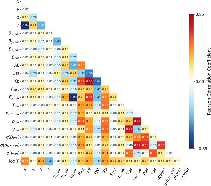
Figure 5. The matrix shows the Pearson correlation coefficients between potential predictors and cold ion flux, $\log (j)$ (left column) rounded to the second decimal.

The cold ion flux does not show clear relations with the SW velocity, in contrast to, for example, for $\sim$100 keV proton flux observed by Kronberg et al. (2020). However, it shows strong increase with the electric field in duskward direction, $E_{y,\text{SW}}$, see Figure 4. The increase in flux is also seen to be correlated with negative $B_{z,\text{IMF}}$, indicating that the IMF topology is a more important factor in triggering the outflow than $v_{\text{SW}}$. A dramatic growth of the flux is observed with the negative $B_{x,\text{IMF}}$ and duskward $B_{y,\text{IMF}}$ components. These imply that the orientation and magnitude of the IMF play a significant role in generation of ion outflow. An enhancement in the cold-ion flux is observed on average with an increase in the variance of SW parameters such as $\sigma (B_{\text{IMF}})$ and $\sigma (n_{H^{+},\text{SW}})$ but not for $\sigma (v_{\text{SW}})$.

3 Model derivation

Here we derive two distinct ML models. For the first approach we use a linear regression (LR) model in order to provide a user-friendly empirical formula to predict the flux of cold ions below 70 eV. For the second approach, we select a nonlinear ML algorithm, which captures nonlinear patterns in the data while improving predictive accuracy.

3.1 Data separation into test and training sets

The dataset is divided using a ”leave-one-year-out” test separation strategy based on an analysis of yearly data distribution and coverage consistency shown in Figure 1. Specifically, data from year 2003 constituted about 19% of the total dataset, aligning well with conventional test set sizes of 20% of total data. The proportion of data points within other years corresponds to either far more or far less than conventional 20% of total data. Another sizing-based candidate is the 2001 data: it accounts for roughly 18% of the data but its temporal coverage is less uniform than that of 2003 (see Figure 1). Therefore, we choose 2003 as our test set to minimize biases stemming from the temporal data coverage. All remaining data is used for the training. Since time is not explicitly included as a predictor in the model we are not using the last 20% of data as the test set to ensure that the training data span both solar-minimum and solar-maximum phases. Although this simple split may yield lower performance compared to other splitting strategies, it creates ”unseen” test dataset conditions.

3.2 Uncertainty quantification and implementation

We evaluate different uncertainties associated with the predictive models. These include point estimates of prediction errors, aleatoric uncertainty arising from data variability, epistemic uncertainty due to model construction, and ensemble uncertainty specific to ensemble-based methods.

3.2.1 Point estimates of model predictions

To assess the performance during training, validation and evaluation processes, we use classical metrics to provide aggregated point estimates of prediction accuracy: the mean squared error (MSE), the root mean squared error (RMSE), the R2-score, the Pearson correlation, the Symmetric Mean Absolute Percentage Error (SMAPE), and the Symmetric Signed Percentage Bias (SSPB). To assess the model improvement of the nonlinear ML model over the linear model, we use the MSE based Skill-score (MSESS). For a detailed metrics description, we refer to the papers by (Morley et al., 2018; Swiger et al., 2022). While these metrics quantify prediction errors, they do not reflect variability or uncertainty inherent of predictions.

3.2.2 Aleatoric (data) uncertainty

In Equation 4, we derived combined relative errors $\delta (j_i)$ for each data point. We implement these relative errors directly into the modeling framework as normalized sample weights $\widehat{w_i}$:

$\widehat{w_i}=\frac{\mathrm{\Delta }{\left(j_i\right)}^{-1}}{{\sum }_{i=1}^n\mathrm{\Delta }{\left(j_i\right)}^{-1}}.(5)$

The weights are applied into the fitting function of the models during the training process, helping to prioritize data points with lower relative errors. Additionally, we incorporate the weights from Equation 5 into evaluation metrics (MSE and R2-score), implementing observational uncertainties within the model’s performance assessment.

3.2.3 Epistemic (model construction) uncertainty

The epistemic uncertainty captures variability in model prediction due to limited training data. To estimate this type of uncertainty, we implement bootstrapping, a method involving 1,000 providing sufficient number of variations) training subsets generated from the original dataset by sampling with replacement. Models are repeatedly trained on these subsets, and their predictions yield distributions from which mean predictions and standard deviations are derived. The bootstrapping mean prediction represents the overall model estimate, while the corresponding standard deviation reflects epistemic uncertainty. This provides us a measure of model sensitivity to changes in training data, quantifying an uncertainty estimation associated with the model building process itself, dependent on the number of bootstrap samples (Weinberger and Sridharan, 2018).

3.2.4 Ensemble and predictor uncertainty (Extra-Trees Regressor model)

For the final model, which is later selected to be Extra-Trees Regressor, the ensemble uncertainty is evaluated by examining prediction variability across the ensemble’s individual decision trees. For each observed data point, we calculate the mean and the standard deviation of predictions generated by all trees in the ensemble. Ensemble variability serves as a measure of the internal consistency and robustness of the model predictions.

The uncertainty contribution of the predictors are assessed using the bootstrapping approach. For each resampled dataset, the ETR model is trained and the resulting feature importances are extracted. From the distributions, we compute the empirical 95% confidence intervals to quantify the variability and robustness of the estimated feature contributions.

3.3 Multicollinearity Analysis and initial feature selection

Multicollinearity among the features can distort coefficient estimates, reduce interpretability, and degrade model performance by inflating parameter variance. Linear models are sensitive to highly correlated predictors. As a measure of linear association, the Pearson correlation coefficient and the Variance Inflation Factor (VIF) help to address this problem. VIF quantifies how much the variance of a coefficient is inflated due to multicollinearity with other predictors, with values above 5 indicating critical multicollinearity (Shrestha, 2020). Strong pairwise Pearson correlations, defined as those exceeding 0.7, can be identified between $x$ and $r$, $n_{H^{+},\text{SW}}$ and $p_{\text{SW}}$, $v_{\text{SW}}$ and $T_{\text{SW}}$, $\text{AE}$ and $\text{Kp}$, and $B_{z,\text{IMF}}$ and $E_{y,\text{SW}}$, see Figure 5. Additionally, several features exhibited VIF values exceeding the threshold of 5: $E_{y,\text{SW}}$, $B_{z,\text{IMF}}$, $p_{\text{SW}}$, $n_{H^{+},\text{SW}}$, $r$ and $\text{Kp}$. Based on these results, $r$ was excluded from the model due to its redundancy with $x$, as it has lower correlation with cold ion flux and a higher VIF. $n_{H^{+},\text{SW}}$ was excluded in favor of $p_{\text{SW}}$ because of its lower correlation with the ion flux and redundancy as $p_{\text{SW}}$ $\propto n_{H^{+},\text{SW}}$. $T_{\text{SW}}$ was excluded in favor of $v_{\text{SW}}$, as SW velocity is more often used in description of the solar wind energy input. $B_{z,\text{IMF}}$ was excluded because of lower correlation with the flux than $E_{y,\text{SW}}$. While the parameters are connected via $E\times B$, we also reduce redundancy for the model. Geomagnetic activity index $\text{Kp}$ was removed due to its lower resolution compared to $\text{AE}$.

For the remaining parameters, the highest Pearson coefficients are below 0.7 and no VIF values exceeded 5. With this, we resolved multicollinearity while preserving the most relevant relationships. Most excluded features are indirectly captured by retained ones. Following this process, we excluded the five parameters, marked by $†$ in Table 1. For both models, we take this remaining feature selection as the basis and individually refine it in both cases, see Section 3.5 and 4.

3.4 Linear regression baseline model

For the first approach, we use multivariate Linear Regression (Neter et al., 1996) by fitting a linear equation to the data that estimates the relationship between a dependent variable, the cold ion flux, and multiple independent variables. The model is fitted using the ordinary least squares (OLS) method, which minimizes the sum of squared residuals to achieve the best linear fit through the data. To derive comparable feature importances for the feature selection process, the model is first trained with predictors, normalized using standard scaler (Pedregosa et al., 2011). Model coefficients derived from normalized input features indicate the relative significance and contributions of individual input features for the models output.

We further refine the selection of the predictors done in Section 3.3 by assessing the performance of the model before and after an exclusion. We use KFold cross-validation (CV), where the training data is split into 5 different subsets. In each step, the model is trained on four subsets and validated on the remaining one. This process provides a fair comparison of a model’s performance across varying data subsets of the original training data. For the linear model we use absolute values for $z$ because of the nonlinear relation with the ion flux, seen in Figure 4.

First, we exclude the remaining geomagnetic indices $\text{Dst}$ and $\text{AE}$ from the feature set. Across the different folds, MSE has shown only a slight increase. In this way, we derive a model that evaluates the flux based on solar input, avoiding the consequences of solar wind-magnetosphere interactions, such as geomagnetic activity. This allows application of the model to exoplanets where we do not measure the magnetic disturbance at the surface. After, we iteratively remove $y$, $v_{\text{SW}}$, $\sigma (v_{\text{SW}})$, $\sigma (n_{H^{+},\text{SW}})$, $B_{x,\text{IMF}}$, $B_{y,\text{IMF}}$, and $\sigma (B_{\text{IMF}})$, which exhibited the lowest scaled coefficients. This leads to slight improvement of the cross-validation performance. The final set of predictors for the linear model is listed as parameters without any symbols such as $\ast$ or $†$ in Table 1.

To derive a predictive formula which can be used with unscaled input data, the model is retrained using the final set of unscaled features. The performance is evaluated on the test dataset from 2003. The corresponding metrics are provided in Table 3 and discussed in Section 4.1.

3.5 Nonlinear model selection

To determine the best performing model for cold ion flux, we evaluate five different ML methods other than linear regression: Extra-Trees Regressor (ETR) (Geurts et al., 2006), Random Forest (Breiman, 2001), Gradient Boosting (Friedman, 2001), Light Gradient Boosting (Ke et al., 2017) (all four ensemble models), and Multi Layer Perceptron (Rumelhart et al., 1986) (neural network). Here we use the models by default settings in combination with the KFold CV. Table 2 presents the CV results obtained for each evaluated model. Among the models, ETR consistently demonstrates the lowest mean CV-MSE (0.17) and the highest Pearson correlation coefficient (66%). Other models exhibit higher mean CV-MSE and lower correlation. Given these results, we select the ETR method to derive a non-linear model for the cold ion flux.

Table 2

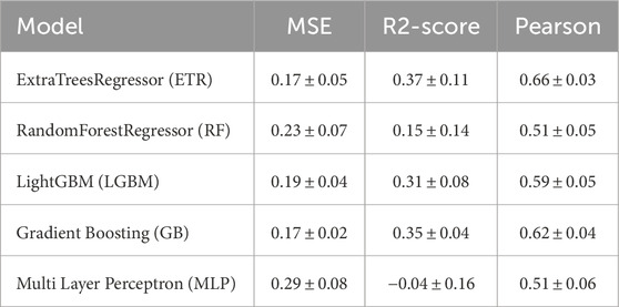
Table 2. Cross-validation performance metrics (mean ± standard deviation) for nonlinear regression models with default settings.

3.6 Extra-trees regressor ensemble model

ETR is a tree based ensemble algorithm. Using bagging, it averages the output of all decision trees (estimators) in the ensemble. Compared to the Random-Forest-Regressor, this method introduces additional randomness by selecting the split thresholds within the decision trees randomly rather than calculating the best feature value threshold. This makes ETR less computationally expensive and also less prone to overfitting. The algorithm selects a random subset of features for each split and trains each tree on the full dataset without bootstrapping. This method is also useful for interpreting the contribution of each individual feature for the predictions such as evaluation of feature importance based on reduction in impurities (Breiman, 2001).

Although the ETR model is not sensitive to multicollinearity, the same feature set as in Section 3.3 is used for consistency across both models. This set is further refined by assessing changes in predictive performance via CV before and after each removal. We first exclude the remaining geomagnetic indices $\text{Dst}$ and $\text{AE}$ from the feature set, as for the linear model (Section 3.4). This resulted in CV performance improvement: both, mean Pearson correlation and mean R2-score increased by 1% while mean MSE remained the same. Subsequently, we attempt further exclusion by removing the least important features from the model. This exclusion resulted in a performance decline, reflected by an increase in the mean CV MSE and decrease in both mean R2-and the Pearson correlation coefficients. Consequently, we decided against further feature reduction. The final set of features comprises of 13 predictors, as those with $\ast$ or without any symbol, listed in Table 1.

We optimize the hyperparameters of the model using Optuna (Akiba et al., 2019), employing a Tree-structured Parzen Estimator (TPE) sampler to efficiently explore a parameter space. The optimization process runs for 500 trials, where each trial evaluates a certain hyperparameter configuration. To assess model performance and generalization, we apply 5-fold CV without shuffle, preserving temporal structure by splitting the training data into five sequential subsets. We optimize four key hyperparameters. The number of estimators controls the number of decision trees in the ensemble, where a higher count generally improves and stabilize the performance but increases computational cost. Here we define a range from 20 to 100. The tree depth is constrained between 5 and 25 to prevent excessive growth of the trees. The minimum number of samples required for a leaf node (between 12 and 40) and the minimum number of samples required for an internal node (between 13 and 40) ensure that splits only occur when there is a sufficient number of samples available. By constraining the model from growing pure leaves, we prevent it from overfitting the training data. After the hyperparameter optimization process, we get a final configuration with 77 estimators, a maximum tree depth of 13, a minimum of 37 samples per leaf, and a minimum of 40 samples per split.

Once the features are selected and the optimal hyperparameters are identified, the final model is trained on the complete training dataset and applied to the test set from 2003 to assess its generalization performance. The metrics are listed in Table 4 and discussed in Section 4.2.

4 Results

4.1 Linear regression results

We derive a predictive formula for the cold ion flux using unscaled features in units provided in Table 1:

$\begin{array}{ll}\hfill {\log }_{10}\left(j\right)& =6.16\cdot 10^{-2}\cdot x-2.90\cdot 10^{-2}\cdot |z|+3.18\cdot 10^{-3}\cdot F10.7\hfill \\ \hfill & +7.14\cdot 10^{-2}\cdot p_{\text{SW}}+4.41\cdot 10^{-2}\cdot E_{y,\text{SW}}+1.19\cdot 10^{-2}\cdot B_{\text{IMF}}\hfill \\ \hfill & +5.35\hfill \end{array}(6)$

The comparison of training and test performance (see Table 3) shows only slight differences, meaning that the model does not have an overfitting problem. On the test set we obtain a predicted mean logarithmic flux value of 5.36 ${\text{cm}}^{-2}{\text{s}}^{-1}$ with RMSE/MAE of 0.44/0.37 ${\text{cm}}^{-2}{\text{s}}^{-1}$. This indicates, that the RMSE difference between the predicted and the measured values is reasonable. The R2-scores of $\sim 40\%$ suggests that a significant portion of the variance remains unexplained by the model. The Pearson correlation coefficients of $\sim 65\%$ shows a significant positive correlation between predicted and observed values of cold ion flux. We observe an increase of the Pearson correlation coefficient and a decrease of the R2-score for the test dataset compared to training dataset. The differences are within expected statistical fluctuations. Such behavior can be related to the simplicity of the approach and the random variability in the data. This aligns with the bias-variance tradeoff, where simpler models tend to have higher bias but lower variance, which leads to comparable performance on both training and test datasets (Hastie et al., 2001). The SMAPE value indicates that, on average, the predictions deviate from the true value by $\sim$6% and $\sim$7%. Low values of the SSPB for both training and test sets suggest that the model generalizes.

Table 3

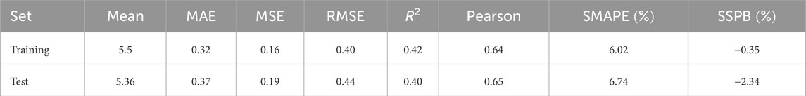
Table 3. Training and test performance-metrics for the linear model.

Figure 6 visualizes the discrepancies between the measured and the predicted cold ion flux values. The predictions are somewhat dispersed, suggesting a model fit that is moderately accurate. The distribution of predicted values indicates a systematic underprediction of high flux values and overprediction of low flux values, particularly towards the extremes. This effect suggests a “regression-to-the-mean” behavior, where the model struggles to capture the full range of variability in the data.

Figure 6

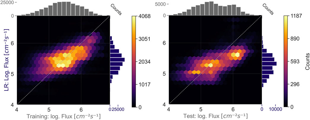
Figure 6. Comparison of measured and LR model predicted cold ion flux, for both training and test datasets. The color bars represent the number of flux values within each bin shown in the plots. The marginal histograms show the distribution of the flux values for both the predicted (vertical) and observed (horizontal) data. A good model predicts most of the fluxes along the white dashed diagonal, namely, closely matching the measurements.

For the test set, the model captures the overall trend in the data. However, it fails to reproduce the bimodal nature of the test data distribution, as shown in the gray histograms in Figure 6. The discrepancy between the measured and predicted values hints to the model’s difficulties in learning and generalizing more intricate nonlinear relationships present in the data.

4.2 Extra-trees-regression results

The ETR model shows a notable improvement in performance compared to the LR model (see Table 4). The RMSE/MAE value of 0.40/0.32 ${\text{cm}}^{-2}{\text{s}}^{-1}$ is lower than that of the LR model and is relatively low compared to the mean logarithmic ion flux value of 5.45 ${\text{cm}}^{-2}{\text{s}}^{-1}$. The R2-score of 50% suggests that the ETR model explains the half of the variance in the data. The Pearson correlation coefficient of 75% indicates a reasonably strong linear relationship between predictions and observations. The SMAPE of the test predictions (6%) indicates high accuracy of prediction. The ability of the ETR model to generalize to unknown data is demonstrated by comparing the values in the training and test metrics, which are not too far apart.

Table 4

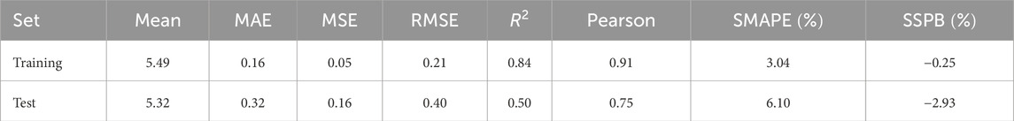
Table 4. Training and test performance metrics for the Extra-Trees Regressor (ETR) model.

Unlike the linear model, which tends to underpredict high flux values and overpredict low flux values, the ETR model better predicts variability in the data. This is reflected by a reduced “regression-to-the-mean-effect”, although it tends to underpredict on the test set (well seen in Figure 7) and indicated by the SSPB of −2.9%. Additionally, the model reproduces the bimodal shape of the test data distribution (see gray histogram), which was not well predicted by the LR model. Overall, the improved metrics indicate that the ETR model is more effective in learning nonlinear relationships in the data.

Figure 7

Figure 7. The two plots compare the measured and ETR model predicted cold ion flux values for both the training and test datasets. The format is the same as in Figure 6.

The feature importance ranking of the ETR model is illustrated in Figure 8. With significant offset the importance ranking in predicting the cold ion flux is led by location parameters $x$ and $z$ followed by $F_{10.7}$. After comes $y$. The next in ranking are features characterising the solar wind: $E_{y,\text{SW}}$, $B_{y,\text{SW}}$, $B_{\text{IMF}}$, $p_{\text{SW}}$, $v_{\text{SW}}$, and $B_{x,\text{SW}}$. Variance-related parameters provide the least contribution to the model’s predictions but still help to improve the performance. More details on physical mechanisms behind the selected parameters is in Section 5.

Figure 8

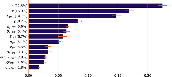
Figure 8. ETR model feature importance values. The length of the orange error bars corresponds to 95% confidence intervals.

Figure 9 demonstrates the predictions of the ETR model during quiet ($\text{Dst}>-30$ nT) and disturbed geomagnetic activity ($\text{Dst}\ge -30$ nT) on the 2003 test dataset. The model tends to underpredict flux values during disturbed geomagnetic activity, with most flux values falling below the white dashed line in Figure 9. For quiet geomagnetic times, overprediction of low flux values and underprediction of mid and high flux values is seen. Performance of the model for quiet conditions exhibits Pearson coefficient of 71%, an R2-Score of 47% and a MSE of 0.16. Under disturbed conditions, the prediction performance improves according to the Pearson correlation of 79%, while MSE and R2-Score values remain the same. The difference in the Pearson correlation may arise from the different data distributions and from the fact, that disturbed cases correspond to only 20% of total test data.

Figure 9

Figure 9. The ETR model predictions for 2003 test data, for quiet (left) and disturbed (right) geomagnetic activity, based on $\text{Dst}$ levels. The format is the same as in Figure 6.

Overall, the Pearson correlation coefficient on the whole 2003 test dataset, seen in Table 4, lies between the results for quiet and disturbed cases. This reflects, that the ETR model provides reliable results under varying geomagnetic conditions.

4.3 Model comparison and uncertainties

As shown in Table 5, the ETR model exhibits slightly higher epistemic uncertainty estimates than the LR model. This is expected because fully deterministic models, such as LR, account less for the variability inherent in the data. Ensemble models such as ETR aggregate multiple estimators and, therefore, capture a wider range of possible values. Additionally, the ensemble uncertainties in the ETR model are higher than the epistemic uncertainties estimated through bootstrapping. This indicates that the variability introduced by combining diverse predictors in the ensemble contributes to the overall uncertainty. However, the aleatoric uncertainty is the highest, if comparing it with epistemic and ensemble uncertainties.

Table 5

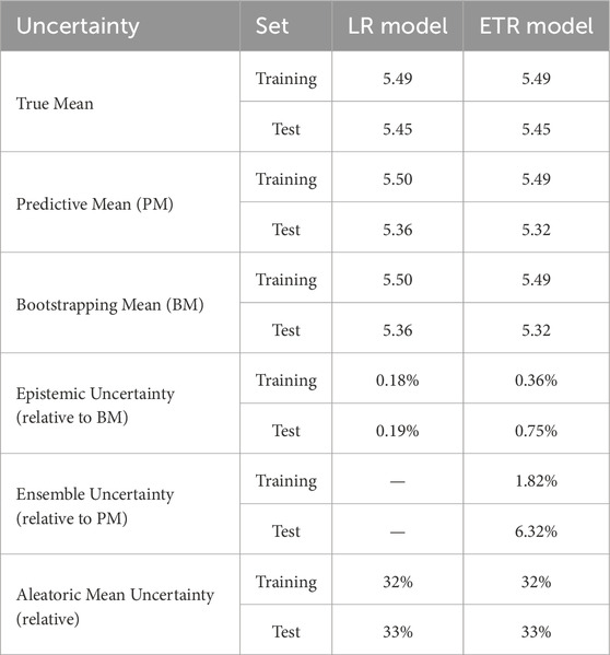
Table 5. Mean cold ion flux values and their specific uncertainties for training and test datasets for LR and ETR models.

We assess the performance improvement of the ETR model compared to the linear baseline model on the unused 2003 test dataset. We use the MSE skill-score (MSESS). This metric provides a quantification of improvement in terms of prediction errors over the linear baseline model (Wheatcroft, 2019). The results show that the ETR model outperforms the linear baseline model in predicting cold ion flux by reducing the prediction error for unseen data by $17\%$. For both, Pearson correlation and R2-score we observe an improvement of 10%.

5 Discussion

5.1 Model performance

Our models show relatively good performance (Pearson scores of 0.65 and 0.75 for the LR and ETR models). Limitations in performance may be due to limited data or the rough data splitting method. However, this splitting strategy may better reflect model generalization across distinct conditions. Both LR and ETR models suffer from “regression-to-the-mean effect”, which results in underprediction of high values and overprediction of the low values. Still, the relative contribution of aleatoric uncertainty is significantly higher than that of epistemic and ensemble uncertainties (see Table 5), indicating that limited measurement precision is a major source of model uncertainty. Although ML models offer powerful tools for uncovering relationships in data, they have limitations. The significance and causality of identified features must be considered cautiously when interpreting the model’s results. ML results do not uncover causal chains in physical processes but suggest statistical relationships that must be validated through physical understanding and further empirical investigation.

5.2 Effects of various parameters on the ion outflow flux

The ETR model identifies spatial variables $x$ and $z$ as the most important predictors of the cold ion flux in the magnetosphere. The flux of cold ions decreases with the radial distance due to the diffusion of particles to a larger volume. Higher flux is observed in the Northern Hemisphere, as seen from Figure 3. This can be explained by the higher ionospheric downward Poynting flux in the Northern Hemisphere according to Yu et al. (2024). Electromagnetic energy that creates a downward Poynting flux controls the ion outflow (Kronberg et al., 2014). The asymmetry may also be related to the weaker magnetic field in this Hemisphere and, consequently, higher electron precipitation. This results in stronger ion outflow; see (Li et al., 2020) for more details. Higher electron precipitation leads to stronger ionospheric conductance (Baumjohann and Treumann, 1996). Indeed, regions with a weaker magnetic field are associated with stronger ionospheric conductance, as shown in the study by Fang (2025). In contrast, a study by Liu et al. (2024) shows that auroral intensity, which is correlated with ion outflow (Kronberg et al., 2014), is weaker in regions with weaker magnetic field. Therefore, the effect of the Earth’s magnetic field on the cold ion outflow is not necessarily straightforward and needs to be addressed in future studies.

Solar EUV irradiance, indicated by the $F_{10.7}$-index, is the most significant factor (after $x$ and $z$) affecting ion outflows according to ETR model (see Figure 8). Solar irradiance changes the ionization rate in the ionosphere modifying the ionospheric density and temperature, and, therefore, the escape rate of the ions (André et al., 2015). A significant correlation was also shown by (Cully et al., 2003; André et al., 2015; Li et al., 2017).

Geomagnetic activity indices such as $\text{AE}$ and $\text{Dst}$ and $\text{Kp}$ have the highest linear correlations with the ion outflow, after $x$ and $z$ (see Figure 5). Geomagnetic activity associated with enhanced charged particle and Poynting flux precipitation leads to the increased ion outflow (Kronberg et al., 2014). Significant correlation of the cold ion outflow with geomagnetic activity is well aligned with the results for geomagnetic storms by (Cully et al., 2003; Li et al., 2012; Li et al., 2013; Goldstein et al., 2018), and for geomagnetic substorms by (Øieroset et al., 1999).

Our goal is to model the outflow based on causal drivers of Sun–Earth interaction (e.g., solar wind parameters) rather than indices of geomagnetic activity, which represent coupled magnetosphere–ionosphere system responses and may both influence and be influenced by ion outflow. This approach also makes it easier or even possible to apply our results to other planets where magnetic activity cannot yet be measured at the surface. We tried LR and ETR models with geomagnetic parameters, but their performance on the training dataset was not significantly better than that of the model driven just by solar parameters.

For the solar wind drivers, we note that $E_{y,\text{SW}}$, $B_{y,\text{IMF}}$, $B_{\text{IMF}}$ and $p_{\text{SW}}$ show the highest contribution to the ETR model (Figure 8). These parameters (excluding $B_{y,\text{IMF}}$) are also used in the LR model and exhibit the highest linear correlations (Figure 4). This demonstrates consistency between the models. Enhanced magnetospheric convection, indicated by $E_{y,\text{SW}}$, is a known driver for ion outflow (Yau and Andre, 1997). $B_{z,\text{IMF}}$ was not included as a model input because it is strongly correlated with $E_{y,\text{SW}}=-V_{x,\text{SW}}\cdot B_{z,\text{IMF}}$. In Figure 4 one can notice strong enhancement of the outflow for negative $B_{z,\text{IMF}}$ and, respectively, positive $E_{y,\text{SW}}$. This magnetic field configuration is effective for the reconnection. In Figure 4 one can also see slight increase of the outflow with increase of positive $B_{z,\text{IMF}}$. This can be explained by reconnection at high latitudes. The reconnection rate also depends on the magnetic field magnitude (Liu et al., 2025). It leads to consequent effective magnetosphere-ionosphere coupling. $B_{y,\text{IMF}}$ defines the location of magnetic reconnection at the magnetopause. The charged particle and Poynting flux generated in this region follow the magnetic field lines and affect the location of the ion outflow in the ionosphere (Liao et al., 2010; Luo et al., 2017). Stronger ion outflow is observed for positive values of $B_{y,\text{IMF}}$ (Figure 4). The asymmetry agrees with the observations by (Howarth and Yau, 2008; Liao et al., 2010; Li et al., 2013) and may reflect larger convection electric field at the dusk side (Howarth and Yau, 2008).

SW dynamic pressure affects the dynamics of the magnetosphere by additional stress on the magnetic field lines at the day side. One of the possible effects is that $p_{\text{SW}}$ also facilitates magnetic reconnection (Kim et al., 2024). A positive correlation between ion outflow and SW dynamic pressure was also reported by Cully et al. (2003).

We examined whether the SW turbulence proxies, such as $\sigma (B_{\text{IMF}})$, $\sigma (n_{H^{+},\text{SW}})$, and $\sigma (v_{\text{SW}})$, are correlated with the cold ion outflow. SW turbulence can be transported to the magnetosphere (Gilder et al., 2020) and can enhance energy transfer to the magnetosphere (Echim et al., 2021). Figure 4 indeed indicates an enhancement of the cold ion flux with increasing turbulence of $\sigma (B_{\text{IMF}})$ and $\sigma (n_{H^{+},\text{SW}})$, but not for $\sigma (v_{\text{SW}})$. The positive relation with $\sigma (B_{\text{IMF}})$ was also found by Cully et al. (2003). However, these parameters are of secondary importance in the ETR model, although the exclusion of these parameters led to a slight decrease in performance.

5.3 Estimation of the cold ion escape rate

The user-friendly linear empirical model in Formula 6 can help us evaluate the total escape rate from the polar cap depending on the variation of solar irradiance and SW dynamic pressure in order to compare their impact. In comparison, the ETR model, while more accurate overall, is less suited for isolating and interpreting the impact of individual parameters. We estimate the polar cap area at the geocentric distance of $\sim$4 ${\text{R}}_E$, as the lowest observations were at this altitude. The edge of the polar cap at this distance can be determined from the first open field lines from the geomagnetic equator for all magnetic longitudes using the Tsyganenko T01 model (Tsyganenko, 2002). The total polar cap area is integrated over all parts of the sphere at different magnetic longitudes. The area was calculated for three activity levels: low, median and high (see Table 6). To run the T01 model, we used $p_{\text{SW}}$, $B_{y,\text{IMF}}$ and $B_{z,\text{IMF}}=-E_{y,\text{SW}}/v_{\text{SW}}$. Furthermore, the $\text{Dst}$ index was taken as 0, -22 and −170 nT for each activity, respectively. This resulted in polar cap areas of $0.61\cdot 10^{15}$, $0.84\cdot 10^{15}$ and $1.33\cdot 10^{15}$ ${\text{m}}^2$, for low, median and high activity, respectively. Note that in case the $\text{Dst}$ index is not available, a simple geometric formula of the polar cap area can be used for a rougher estimation. The values of the input parameters in Formula 6 are listed in Table 6. For each activity level, we vary either $F_{10.7}$ or $p_{\text{SW}}$. The results are shown in Figure 10. We can see that the solar irradiance and the SW pressure strongly modulate the outward fluence. This means that the contribution of stellar wind-magnetosphere coupling along with the stellar irradiance has to be considered in modeling the ion outflow at Earth and Earth-like exoplanets. The LR model can help estimate the influence of such an interaction on the ion outflow at exoplanets. The outward fluence varies over approximately three orders of magnitude, from $\sim 1.1\times 10^{24}$ to $\sim 2.7\times 10^{26}$ ions/s, with median value $\sim 7\times 10^{24}$. The fluences estimated in previous studies, such as, $\sim$0.2-$1\times 10^{26}$ ions/s by André and Cully (2012) and an upper limit of $\sim 3\times 10^{26}$ ions/s for 10–30 eV oxygen from Strangeway et al. (2005), are similar to the high activity values predicted by our model. The upper limit is comparable with the atmospheric neutral hydrogen escape related to Jeans process for the solar maximum, which is $\sim 6\times 10^{26}$ ions/s and the charge-exchange escape of neutrals for the solar minimum $\sim 6\times 10^{26}$ ions/s (Gronoff et al., 2020). However, the estimated escape rate is only a part of the total ion outflow from the polar cap. To evaluate the total outflow rate, particles with energies above 70 eV and ion species other than hydrogen must also be considered. This means that the contribution of the cold ion outflow in the total atmospheric escape, according to LR, is not negligible during active solar wind conditions. The fluence values for the ETR model are $\sim 4.9\times 10^{24}$, $\sim 6.1\times 10^{24}$ and $\sim 2\times 10^{25}$ for low, median, and high activity levels, respectively. The values are lower than those derived by the LR model and in previous studies. This may be due to the tendency of the ETR model to underpredict high flux values, as shown in Figure 7.

Table 6

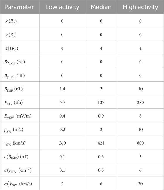
Table 6. Parameters for low-, mid (median)- and high-activity levels used to calculate outward fluence with Formula 6, depicted in Figure 10.

Figure 10

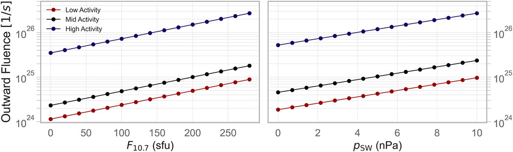
Figure 10. Total escape rate profiles of cold ions ($<$70 eV) from the dipole polar cap area for three activity levels, with a maximum outflow range of $1.1\cdot 10^{24}$ to $2.7\cdot 10^{26}$ ions/s, shown as a function of solar EUV irradiance (left) and solar wind pressure (right).

6 Conclusions and outlook

In this work we used Cluster measurements to derive models for cold ion outflow. We developed a linear model with empirical formula and a more accurate nonlinear ensemble model to predict cold ion flux in the magnetospheric lobes for particles emanating from Earth’s ionosphere. The models use solar activity parameters as predictors. The spatial variables $x$ and $z$ are the most important predictors for the cold ion flux. The flux decreases with altitude, an expected effect due to ion diffusion into a larger volume, and a north-south asymmetry is observed. According to the ETR model, solar EUV irradiance, indicated by $F_{10.7}$, is the most significant solar activity parameter. Among the solar wind drivers, $E_{y,\text{SW}}$, $B_{y,\text{IMF}}$, $B_{\text{IMF}}$ and $p_{\text{SW}}$ show mainly the highest linear correlations with the cold ion flux and highest contribution as predictors to the nonlinear model. The importance of these parameters indicates the effectiveness of the solar-wind-magnetopshere-ionosphere coupling and of reconnection in triggering cold ion outflow. We estimate the total escape rate range of cold ions ($<$70 eV) from the polar cap to be between $\sim 1.1\times 10^{24}$ ions/s and $\sim 2.7\times 10^{26}$ ions/s, which is comparable to the neutral escape for the high activity. To estimate the total ion outflow, contributions from higher energies must be included. The derived linear model can help to scale the influence of the stellar wind magnetospheric interaction on the ion outflow at Earth-like exoplanets.

In future studies, we plan to extend the database of cold ion fluxes, to include additional input parameters such as temporal history, solar wind energy, X-ray flux, magnetopause location, and terrestrial magnetic field. We will also consider more advanced feature engineering for the linear baseline model.

Data availability statement

The datasets used in this research are available in the following repositories: the Cluster Science Archive at https://csa.esac.esa.int/csa-web/ and the NASA OMNIWeb http://omniweb.gsfc.nasa.gov/. The model files are provided in the Zenodo Open Access repository {https://doi.org/10.5281/zenodo.17288188}. The software packages used, including Sklearn (Pedregosa et al., 2011b), Numpy (Harris et al., 2020), Pandas (The pandas development team, 2020), Matplotlib (Hunter, 2007), Optuna (Akiba et al., 2019b) and Seaborn (Waskom, 2021).

Author contributions

ND: Validation, Writing – original draft, Visualization, Formal Analysis, Writing – review and editing, Investigation, Conceptualization, Software, Methodology. EK: Investigation, Funding acquisition, Formal Analysis, Validation, Methodology, Writing – original draft, Supervision, Conceptualization, Writing – review and editing, Project administration. KL: Resources, Writing – review and editing, Formal Analysis, Data curation. AS: Formal Analysis, Writing – review and editing. RI: Formal Analysis, Writing – review and editing. FS: Writing – review and editing, Formal Analysis.

Funding

The author(s) declare that financial support was received for the research and/or publication of this article. EK and ND are supported by the German Research Foundation (DFG) under GZ KR 4375/2-1 within SPP “Dynamic Earth”. EK is also funded by the DFG Heisenberg grant under number 516641019. Additionally, AS and ND are supported by DFG project number 520916080. EK, ND and KL acknowledge the LMU-China Academic Network for the support. Work at the University of Illinois at Urbana-Champaign was performed with financial support from the NASA grant 80NSSC24K0273.

Acknowledgments

We acknowledge Mats André and Anders Eriksson for their invaluable input on cold ion observations. We also grateful to Mei-Yun Lin, Kevin Heng and Simon Mischel for useful discussions.

Conflict of interest

The authors declare that the research was conducted in the absence of any commercial or financial relationships that could be construed as a potential conflict of interest.

The author(s) declared that they were an editorial board member of Frontiers, at the time of submission. This had no impact on the peer review process and the final decision.

Generative AI statement

The author(s) declare that no Generative AI was used in the creation of this manuscript.

Any alternative text (alt text) provided alongside figures in this article has been generated by Frontiers with the support of artificial intelligence and reasonable efforts have been made to ensure accuracy, including review by the authors wherever possible. If you identify any issues, please contact us.

Publisher’s note

All claims expressed in this article are solely those of the authors and do not necessarily represent those of their affiliated organizations, or those of the publisher, the editors and the reviewers. Any product that may be evaluated in this article, or claim that may be made by its manufacturer, is not guaranteed or endorsed by the publisher.

References

Akiba, T., Sano, S., Yanase, T., Ohta, T., and Koyama, M. (2019). “Optuna: a next-generation hyperparameter optimization framework,” in Proceedings of the 25th ACM SIGKDD International Conference on Knowledge Discovery & Data Mining, 2623–2631doi. doi:10.1145/3292500.3330701

CrossRef Full Text | Google Scholar

André, M., and Cully, C. M. (2012). Low-energy ions: a previously hidden solar system particle population. Geophys. Res. Lett. 39. doi:10.1029/2011GL050242

CrossRef Full Text | Google Scholar

André, M., Li, K., and Eriksson, A. I. (2015). Outflow of low-energy ions and the solar cycle. J. Geophys. Res. Space Phys. 120, 1072–1085. doi:10.1002/2014JA020714

CrossRef Full Text | Google Scholar

André, M., Eriksson, A. I., Khotyaintsev, Y. V., and Toledo-Redondo, S. (2021). The spacecraft wake: interference with electric field observations and a possibility to detect cold ions. J. Geophys. Res. Space Phys. 126, e29493. doi:10.1029/2021JA029493

CrossRef Full Text | Google Scholar

Balogh, A., Carr, C. M., Acuña, M. H., Dunlop, M. W., Beek, T. J., Brown, P., et al. (2001). The cluster magnetic field investigation: overview of in-flight performance and initial results. Ann. Geophys. 19, 1207–1217. doi:10.5194/angeo-19-1207-2001

CrossRef Full Text | Google Scholar

Baumjohann, W., and Treumann, R. A. (1996). Basic space plasma physics.

Google Scholar

Breiman, L. (2001). Random forests. Random For. 45, 5–32. doi:10.1023/A:1010933404324

CrossRef Full Text | Google Scholar

Chappell, C. R., Moore, T. E., and Waite, Jr., J. H. (1987). The ionosphere as a fully adequate source of plasma for the earth’s magnetosphere. J. Geophys. Res. Space Phys. 92, 5896–5910. doi:10.1029/JA092iA06p05896

CrossRef Full Text | Google Scholar

Cully, C. M., Donovan, E. F., Yau, A. W., and Arkos, G. G. (2003). Akebono/suprathermal mass spectrometer observations of low-energy ion outflow: dependence on magnetic activity and solar wind conditions. J. Geophys. Res. Space Phys. 108. doi:10.1029/2001JA009200

CrossRef Full Text | Google Scholar

Davis, T. N., and Sugiura, M. (1966). Auroral electrojet activity index ae and its universal time variations. J. Geophys. Res. (1896-1977) 71, 785–801. doi:10.1029/JZ071i003p00785

CrossRef Full Text | Google Scholar

Delzanno, G. L., Borovsky, J. E., Henderson, M. G., Resendiz Lira, P. A., Roytershteyn, V., and Welling, D. T. (2021). The impact of cold electrons and cold ions in magnetospheric physics. J. Atmos. Solar-Terrestrial Phys. 220, 105599. doi:10.1016/j.jastp.2021.105599

CrossRef Full Text | Google Scholar

Echim, M., Chang, T., Kovacs, P., Wawrzaszek, A., Yordanova, E., Narita, Y., et al. (2021). “Turbulence and complexity of magnetospheric plasmas,” in Magnetospheres in the solar system. Editors R. Maggiolo, N. André, H. Hasegawa, and D. T. Welling 2, 67–91. doi:10.1002/9781119815624.ch5

CrossRef Full Text | Google Scholar

Engwall, E., Eriksson, A. I., André, M., Dandouras, I., Paschmann, G., Quinn, J., et al. (2006). Low-energy (order 10 ev) ion flow in the magnetotail lobes inferred from spacecraft wake observations. Geophys. Res. Lett. 33. doi:10.1029/2005GL025179

CrossRef Full Text | Google Scholar

Engwall, E., Eriksson, A. I., Cully, C. M., André, M., Torbert, R., and Vaith, H. (2008). Earth’s ionospheric outflow dominated by hidden cold plasma. Nat. Geosci. 2, 24–27. doi:10.1038/ngeo387

CrossRef Full Text | Google Scholar

Engwall, E., Eriksson, A. I., Cully, C. M., André, M., Puhl-Quinn, P. A., Vaith, H., et al. (2009). Survey of cold ionospheric outflows in the magnetotail. Ann. Geophys. 27, 3185–3201. doi:10.5194/angeo-27-3185-2009

CrossRef Full Text | Google Scholar

Escoubet, C., Fehringer, M., and Goldstein, M. (2001). IntroductionThe cluster mission. Ann. Geophys. 19, 1197–1200. doi:10.5194/angeo-19-1197-2001

CrossRef Full Text | Google Scholar

Fang, X. (2025). A new fast calculation method for pedersen and hall conductances from maxwellian electron precipitation: incorporating magnetic field dependence. J. Geophys. Res. Space Phys. 130, e2025JA033835. doi:10.1029/2025JA033835

CrossRef Full Text | Google Scholar

Friedman, J. H. (2001). Greedy function approximation: a gradient boosting machine. Ann. statistics 29, 1189–1232. doi:10.1214/aos/1013203451

CrossRef Full Text | Google Scholar

Geurts, P., Ernst, D., and Wehenkel, L. (2006). Extremely randomized trees. Mach. Learn. 63, 3–42. doi:10.1007/s10994-006-6226-1

CrossRef Full Text | Google Scholar

Gilder, S., Wack, M. R., Kronberg, E. A., and Prabhu, A. (2020). Geomagnetism, aeronomy and space weather. Cambridge University Press, 71–83.

Google Scholar

Goldstein, J., Llera, K., McComas, D. J., Redfern, J., and Valek, P. W. (2018). Empirical characterization of low-altitude ion flux derived from twins. J. Geophys. Res. Space Phys. 123, 3672–3691. doi:10.1029/2017JA024957

CrossRef Full Text | Google Scholar

Gronoff, G., Arras, P., Baraka, S., Bell, J. M., Cessateur, G., Cohen, O., et al. (2020). Atmospheric escape processes and planetary atmospheric evolution. J. Geophys. Res. Space Phys. 125, e2019JA027639. doi:10.1029/2019ja027639

CrossRef Full Text | Google Scholar

Gustafsson, G., André, M., Carozzi, T., Eriksson, A. I., Fälthammar, C.-G., Grard, R., et al. (2001). First results of electric field and density observations by cluster efw based on initial months of operation. Ann. Geophys. 19, 1219–1240. doi:10.5194/angeo-19-1219-2001

CrossRef Full Text | Google Scholar

Harris, C. R., Millman, K. J., van der Walt, S. J., Gommers, R., Virtanen, P., Cournapeau, D., et al. (2020). Array programming with numpy. Nature 585, 357–362. doi:10.1038/s41586-020-2649-2

PubMed Abstract | CrossRef Full Text | Google Scholar

Hastie, T., Tibshirani, R., and Friedman, J. (2001). The elements of statistical learning springer series in statistics. New York, NY, USA: Springer New York Inc.

Google Scholar

Howarth, A., and Yau, A. W. (2008). The effects of IMF and convection on thermal ion outflow in magnetosphere-ionosphere coupling. J. Atmos. Solar-Terrestrial Phys. 70, 2132–2143. doi:10.1016/j.jastp.2008.08.008

CrossRef Full Text | Google Scholar

Hunter, J. D. (2007). Matplotlib: a 2d graphics environment. Comput. Sci. & Eng. 9, 90–95. doi:10.1109/MCSE.2007.55

CrossRef Full Text | Google Scholar

Ke, G., Meng, Q., Finley, T., Wang, T., Chen, W., Ma, W., et al. (2017). Lightgbm: a highly efficient gradient boosting decision tree. Adv. neural Inf. Process. Syst. 30, 3146–3154. doi:10.5555/3294996.3295074

CrossRef Full Text | Google Scholar

Kim, H., Connor, H. K., Zou, Y., Park, J., Nakamura, R., and McWilliams, K. (2024). Relation between magnetopause position and reconnection rate under quasi-steady solar wind dynamic pressure. Earth, Planets Space 76, 165. doi:10.1186/s40623-024-02101-9

PubMed Abstract | CrossRef Full Text | Google Scholar

King, J. H., and Papitashvili, N. E. (2005). Solar wind spatial scales in and comparisons of hourly wind and ace plasma and magnetic field data. J. Geophys. Res. Space Phys. 110. doi:10.1029/2004JA010649

CrossRef Full Text | Google Scholar

Kronberg, E. A., Ashour-Abdalla, M., Dandouras, I., Delcourt, D. C., Grigorenko, E. E., Kistler, L. M., et al. (2014). Circulation of heavy ions and their dynamical effects in the magnetosphere: recent observations and models. Space Sci. Rev. 184, 173–235. doi:10.1007/s11214-014-0104-0

CrossRef Full Text | Google Scholar

Kronberg, E. A., Gastaldello, F., Haaland, S., Smirnov, A., Berrendorf, M., Ghizzardi, S., et al. (2020). Prediction and understanding of soft-proton contamination in XMM-Newton: a machine learning approach. Astrophysical J. 903, 89. doi:10.3847/1538-4357/abbb8f

CrossRef Full Text | Google Scholar

Kronberg, E. A., Grigorenko, E. E., Ilie, R., Kistler, L., and Welling, D. (2021). “Impact of ionospheric ions on magnetospheric dynamics,” in Geophysical monograph series. Editors R. Maggiolo, N. André, H. Hasegawa, D. T. Welling, Y. Zhang, and L. J. Paxton 1 edn. (Wiley), 353–364. doi:10.1002/9781119815624.ch23

CrossRef Full Text | Google Scholar

Li, K., Haaland, S., Eriksson, A., André, M., Engwall, E., Wei, Y., et al. (2012). On the ionospheric source region of cold ion outflow. Geophys. Res. Lett. 39, L18102. doi:10.1029/2012GL053297

CrossRef Full Text | Google Scholar

Li, K., Haaland, S., Eriksson, A., André, M., Engwall, E., Wei, Y., et al. (2013). Transport of cold ions from the polar ionosphere to the plasma sheet. J. Geophys. Res. Space Phys. 118, 5467–5477. doi:10.1002/jgra.50518

CrossRef Full Text | Google Scholar

Li, K., Wei, Y., André, M., Eriksson, A., Haaland, S., Kronberg, E. A., et al. (2017). Cold ion outflow modulated by the solar wind energy input and tilt of the geomagnetic dipole. J. Geophys. Res. Space Phys. 122 (10), 658–668. doi:10.1002/2017JA024642

CrossRef Full Text | Google Scholar

Li, K., Förster, M., Rong, Z., Haaland, S., Kronberg, E., Cui, J., et al. (2020). The polar wind modulated by the spatial inhomogeneity of the strength of the earth’s magnetic field. J. Geophys. Res. Space Phys. 125, e2020JA027802. doi:10.1029/2020ja027802

CrossRef Full Text | Google Scholar

Liao, J., Kistler, L. M., Mouikis, C. G., Klecker, B., Dandouras, I., and Zhang, J.-C. (2010). Statistical study of o+ transport from the cusp to the lobes with cluster codif data. J. Geophys. Res. Space Phys. 115. doi:10.1029/2010JA015613

CrossRef Full Text | Google Scholar

Liu, Z.-Y., Zong, Q.-G., Li, L., Feng, Z.-J., Sun, Y.-X., Yu, X.-Q., et al. (2024). The impact of the south atlantic anomaly on the aurora system. Geophys. Res. Lett. 51, e2023GL107209. doi:10.1029/2023GL107209

CrossRef Full Text | Google Scholar

Liu, Y.-H., Hesse, M., Genestreti, K., Nakamura, R., Burch, J. L., Cassak, P. A., et al. (2025). Ohm’s law, the reconnection rate, and energy conversion in collisionless magnetic reconnection. Space Sci. Rev. 221, 16. doi:10.1007/s11214-025-01142-0

PubMed Abstract | CrossRef Full Text | Google Scholar

Luo, H., Kronberg, E. A., Nykyri, K., Trattner, K. J., Daly, P. W., Chen, G. X., et al. (2017). IMF dependence of energetic oxygen and hydrogen ion distributions in the near-Earth magnetosphere. J. Geophys. Res. Space Phys. 122, 5168–5180. doi:10.1002/2016JA023471

CrossRef Full Text | Google Scholar

Lybekk, B., Pedersen, A., Haaland, S., Svenes, K., Fazakerley, A. N., Masson, A., et al. (2012). Solar cycle variations of the cluster spacecraft potential and its use for electron density estimations. J. Geophys. Res. Space Phys. 117. doi:10.1029/2011JA016969

CrossRef Full Text | Google Scholar

Matzka, J., Stolle, C., Yamazaki, Y., Bronkalla, O., and Morschhauser, A. (2021). The geomagnetic kp index and derived indices of geomagnetic activity. Space weather. 19, e2020SW002641. doi:10.1029/2020SW002641

CrossRef Full Text | Google Scholar

Morley, S. K., Brito, T. V., and Welling, D. T. (2018). Measures of model performance based on the log accuracy ratio. Space weather. 16, 69–88. doi:10.1002/2017SW001669

CrossRef Full Text | Google Scholar

Neter, J., Kutner, M. H., Nachtsheim, C. J., and Wasserman, W. (1996). Applied linear statistical models (Chicago: Irwin)

Google Scholar

Nose, M., Iyemori, T., Sugiura, M., and Kamei, T. (2015). Geomagnetic ae index. doi:10.17593/15031-54800

CrossRef Full Text | Google Scholar

Øieroset, M., Yamauchi, M., Liszka, L., and Hultqvist, B. (1999). Energetic ion outflow from the dayside ionosphere: categorization, classification, and statistical study. J. Geophys. Res. Space Phys. 104, 24915–24927. doi:10.1029/1999JA900248

CrossRef Full Text | Google Scholar

Paschmann, G., Melzner, F., Frenzel, R., Vaith, H., Parigger, P., Pagel, U., et al. (1997). The electron drift instrument for cluster. Space Sci. Rev. 79, 233–269. doi:10.1023/a:1004917512774

CrossRef Full Text | Google Scholar

Pedersen, A., Lybekk, B., André, M., Eriksson, A., Masson, A., Mozer, F. S., et al. (2008). Electron density estimations derived from spacecraft potential measurements on cluster in tenuous plasma regions. J. Geophys. Res. Space Phys. 113. doi:10.1029/2007JA012636

CrossRef Full Text | Google Scholar

Pedregosa, F., Varoquaux, G., Gramfort, A., Michel, V., Thirion, B., Grisel, O., et al. (2011). Scikit-learn: machine learning in python. J. Mach. Learn. Res. 12, 2825–2830. doi:10.48550/arXiv.1201.0490

CrossRef Full Text | Google Scholar

Rumelhart, D. E., Hinton, G. E., and Williams, R. J. (1986). Learning representations by back-propagating errors. Nature 323, 533–536. doi:10.1038/323533a0

CrossRef Full Text | Google Scholar

Shrestha, N. (2020). Detecting multicollinearity in regression analysis. Am. J. Appl. Math. Statistics 8, 39–42. doi:10.12691/ajams-8-2-1

CrossRef Full Text | Google Scholar

Strangeway, R. J., Ergun, R. E., Su, Y.-J., Carlson, C. W., and Elphic, R. C. (2005). Factors controlling ionospheric outflows as observed at intermediate altitudes. J. Geophys. Res. Space Phys. 110. doi:10.1029/2004JA010829

CrossRef Full Text | Google Scholar

Sugiura, M. (1964). Hourly values of equatorial dst for the igy. Ann. Int. Geophys. 35, 9–45.

Google Scholar

Swiger, B. M., Liemohn, M. W., Ganushkina, N. Y., and Dubyagin, S. V. (2022). Energetic electron flux predictions in the near-earth plasma sheet from solar wind driving. Space Weather 20, e2022SW003150. doi:10.1029/2022SW003150

CrossRef Full Text | Google Scholar

Tapping, K. F. (2013). The 10.7 cm solar radio flux (f10.7). Space weather 11, 394–406. doi:10.1002/swe.20064

CrossRef Full Text | Google Scholar

The pandas development team (2020). pandas-dev/pandas: Pandas. Zenodo. doi:10.5281/zenodo.3509134

CrossRef Full Text | Google Scholar

Toledo-Redondo, S., André, M., Aunai, N., Chappell, C. R., Dargent, J., Fuselier, S. A., et al. (2021). Impacts of ionospheric ions on magnetic reconnection and earth’s magnetosphere dynamics. Rev. Geophys. 59, e00707. doi:10.1029/2020RG000707

CrossRef Full Text | Google Scholar

Tsyganenko, N. A. (2002). A model of the near magnetosphere with a dawn-dusk asymmetry 1. mathematical structure. J. Geophys. Res. Space Phys. 107 (SMP 12–1), 12–15. doi:10.1029/2001JA000219

CrossRef Full Text | Google Scholar

Waskom, M. L. (2021). Seaborn: statistical data visualization. J. Open Source Softw. 6, 3021. doi:10.21105/joss.03021

CrossRef Full Text | Google Scholar

Weinberger, K. Q., and Sridharan, K. (2018). Cs4780/cs5780: machine learning for intelligent systems. Lecture notes.

Google Scholar

Welling, D. T., André, M., Dandouras, I., Delcourt, D., Fazakerley, A., Fontaine, D., et al. (2015). The earth: plasma sources, losses, and transport processes. Space Sci. Rev. 192, 145–208. doi:10.1007/s11214-015-0187-2

CrossRef Full Text | Google Scholar

Wheatcroft, E. (2019). Interpreting the skill score form of forecast performance metrics. Int. J. Forecast. 35, 573–579. doi:10.1016/j.ijforecast.2018.11.010

CrossRef Full Text | Google Scholar

Yau, A. W., and Andre, M. (1997). Sources of ion outflow in the high latitude ionosphere. Space Sci. Rev. 80, 1–25. doi:10.1023/A:1004947203046

CrossRef Full Text | Google Scholar

Yu, C., Zhang, X.-X., Wang, W., and He, F. (2024). Hemispheric asymmetry of ionospheric poynting flux during geomagnetically quiet periods. J. Geophys. Res. Space Phys. 129, e2024JA032519. doi:10.1029/2024JA032519

CrossRef Full Text | Google Scholar