Propagation of whistler mode waves in Earth’s inner magnetosphere in the presence of field aligned irregularities and geomagnetic curvature

Whistler mode waves are known to propagate in the Earth’s magnetosphere along complex trajectories and have a significant impact on space weather processes and radiation belt energy dynamics. Most past work on propagation trajectories of whistler mode waves has been done using ray tracing, which is appropriate for smoothly varying background plasma densities. Recent spacecraft observations suggest that the cold plasma density in the magnetosphere can often be highly inhomogeneous. In this study, we investigate the propagation of whistler mode waves in cold, inhomogeneous plasma, with a focus on the combined effects of geomagnetic curvature and density irregularities known as magnetospheric ducts. Using both a comprehensive full wave model and a ray tracing model, we simulate wave behavior under conditions representative of Van Allen Probe observations. The presence of magnetospheric ducts produces a more complex wave behavior in the full wave model, leading to a strong spatial modulation, efficient confinement and the formation of shadow region as a result of geomagnetic curvature. The ray tracing simulation provides a complementary perspective, highlighting the propagation paths of individual rays in the background cold plasma density and, demonstrates the reflection, bending and guiding of rays due to density gradients. Employing both of these models provides insight into the effects of density ducts in the whistler mode wave propagation and understanding of the wave power distribution in global magnetospheric models.

1 Introduction

Electromagnetic waves in the Extremely Low Frequency (ELF, 300 Hz–3 kHz) and Very Low Frequency (VLF, 3–30 kHz) band propagate in the Earth’s magnetosphere as whistler mode plasma waves and play an important role in near-Earth space weather, regulating the dynamics of the outer radiation belts (Inan et al., 1985; Abel and Thorne, 1998; Meredith et al., 2006). Of particular interest is the generation and propagation of magnetospherically generated whistler-mode waves known as chorus and hiss. Chorus is well-known to play a pivotal role in acceleration and losses of energetic electrons in the outer radiation belt (Bortnik and Thorne, 2007). Chorus waves are generated near the geomagnetic equator outside the plasmasphere typically with quasi-parallel wave normal angle (WNA) $\theta -$ the angle between the wave normal vector and the background magnetic field direction (Agapitov et al., 2011b; Agapitov et al., 2011a; Agapitov et al., 2013; Bortnik et al., 2011; Yearby et al., 2011; Breuillard et al., 2012; Chen et al., 2014). Propagating to higher latitudes, whistler mode WNAs increase due to curvature of the geomagnetic field lines, and in the absence of local amplification and damping, approximately follow a linear dependence (Agapitov et al., 2013). However, it is known that plasma density anisotropic inhomogeneities can significantly affect propagation of whistler mode waves leading to more field aligned WNAs and spatial modulation of wave amplitude (Hanzelka and Santolík, 2019; Hosseini et al., 2021; Ke et al., 2021; Zhang et al., 2024)

The most common methodology for modeling the propagation of chorus waves within the magnetosphere is ray tracing (Kimura, 1966; Inan and Bell, 1977; Maxworth and Golkowski, 2017; Pasmanik and Demekhov, 2017; Maxworth et al., 2020). The ray tracing approximation has been successful in explaining various observed phenomena such as magnetospheric reflection (MR) of lightning-whistlers (Bortnik et al., 2003) and propagation of chorus into the plasmasphere (Bortnik et al., 2008). In a smooth magnetosphere, the ray tracing approximation predicts a linear increase in WNA with latitude for chorus waves generated at the equator (Breuillard et al., 2012; Chen et al., 2014; Pasmanik and Demekhov, 2020). However, observations show that at high latitudes, the WNA does not always increase as expected and the waves are more parallel propagating than predicted from ray tracing in a smooth magnetosphere (Agapitov et al., 2011a; Agapitov et al., 2015; Agapitov et al., 2018; Hanzelka and Santolík, 2022). This contradiction suggests the possibility of field aligned density irregularities being important. When field aligned irregularities extend over several degrees of latitude, they are often called magnetospheric “ducts.” Such ducts can effectively guide whistler-mode waves to high latitudes and enforce parallel propagation (Gołkowski and Inan, 2008; Pasmanik and Demekhov, 2020). Although ray tracing has been used to model a range of duct dimensions compared to a wavelength, the equations are formally invalid for density changes that approach single wavelength scales. Under these considerations, a full wave technique is required to model the propagation of whistler mode waves in plasmas with small scale density inhomogeneities (Streltsov et al., 2006; 2007; Katoh, 2014; Zudin et al., 2019).

Recent spacecraft observations confirm the existence of field aligned plasma density irregularities and their strong influence on observed whistler mode wave parameters (Hanzelka and Santolík, 2019; Chen et al., 2021; Hosseini et al., 2021; Harid et al., 2024; Zhang et al., 2024). Figure 1 shows examples of observations on the Van Allen Probes A (also known as Radiation Belt Storm Probe A) spacecraft that exhibits a significant density irregularity region and simultaneous wave power enhancement. These observations are readily interpreted as ducting of the whistler mode waves that originate from an equatorial source. The density irregularities exhibit both large scale (>100 km) and small scale (<20 km) features. Although the concept of ducts and cold plasma inhomogeneities guiding waves is not new (Smith et al., 1960; Inan and Bell, 1977; Sonwalkar et al., 1994), the effect of such irregularities on observable wave parameters remains a topic of active study (Hanzelka and Santolík, 2019; 2022; Hosseini et al., 2020; Pasmanik and Demekhov, 2020; Chen et al., 2021; Williams and Streltsov, 2021; Harid et al., 2024).

Figure 1

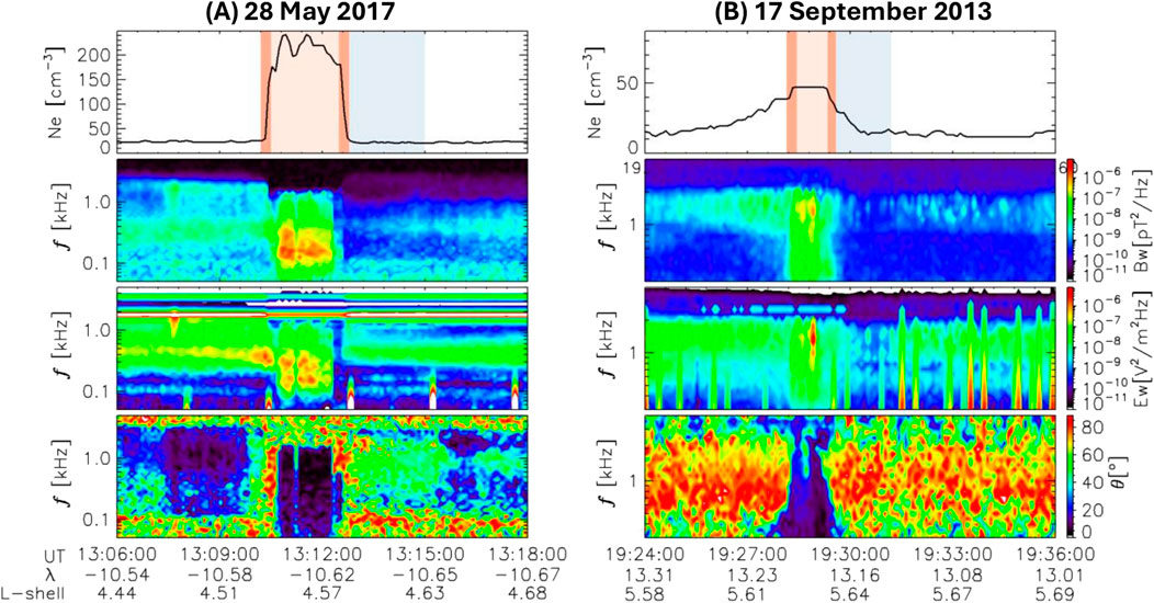
Figure 1. Two density irregularity region incidents crossing recorded by VAPA (Van Allen Probes A): (A) 28 May 2017 (left); (B) 17 September 2013 (right). The panels from top to bottom present the plasma density, the magnetic field dynamics spectrum, the electric field dynamic spectrum, and the wave normal angle (WNA) where λ indicates the magnetic latitude.

Two examples of observed duct-like structures crossing are shown in Figure 1 where the horizontal axes show the position of the space craft in time, magnetic latitude, $\lambda$, and L shell. The WNAs of whistler waves inside the duct are more field aligned than WNAs outside the structure. For case #1 in Figure 1A, WNAs observed before the spacecraft crosses the density inhomogeneity were about 20–25°, i.e., about twice of the magnetic latitude, indicating propagation from the source, where waves are assumed to be field aligned, in line with that predicted by raytracing in homogenous but anisotropic medium (Agapitov et al., 2013). In the vicinity of duct boundaries, the WNA becomes very oblique (up to 80°). We can identify four regions with unique behavior of WNAs around the large scale density intense duct at intermediate $\lambda$: (1) the unperturbed region with WNA well explained by the raytracing in a constant background density; (2) the duct boundary regions with very oblique WNAs (marked in dark red in the top panels of Figure 1); (3) the duct region with field aligned WNAs (highlighted as a light red region in the top panels of Figure 1); (4) the duct “shadow” region at higher L-shells with sudden increase (∼45–55°) of WNAs and significant depletion of wave amplitude (wave magnetic field perturbation goes down to almost the background noise level which is represented by a light blue region in the top panels of Figure 1). Case #2 in Figure 1B shows propagation of hiss waves near the equator, with waves outside the duct having very oblique WNA (around 70–80°), and only inside the duct is the field aligned propagation observed. In case #2, we can identify only three regions from the four listed above: the unperturbed region; the duct region, and the shadow region.

In this work, we use both raytracing and a finite difference time domain (FDTD) model to investigate the effects of whistler mode waves propagation in a dipole magnetic field (the geomagnetic dipole) with plasma density inhomogeneities like those observed on spacecraft and presented in Figure 1A. To rigorously analyze the observational data, we simulate both the ray tracing and FDTD models in the presence of ducts. Section 2 presents the theoretical background of the models, and the simulation setup. Comparison of the numerical results with observations of whistler waves propagating in a smooth magnetosphere and density enhancement ducts is presented in Section 3 and Section 4. A summary and conclusions are presented in Section 5.

2 Theoretical background of models

2.1 Ray tracing model

Ray tracing theory was first applied to whistler mode waves in the magnetosphere by Kimura (1966) and uses the index of refraction and Snell’s law to develop the ray path under various inhomogeneous and anisotropic conditions. This allows for tracing of the trajectories of waves as wave packets. However, the ray tracing model requires the assumption that the index of refraction does not vary significantly over a wavelength. The raytracing algorithm tracks the change in wave vector that is dependent on both the position of the wave and time. Consequently, the change in wave vector, along with the change in position and wave velocity, can be determined. The dispersion function of the cold plasma for the ray tracing simulations given by

$\mathit{D}\left(\mathit{\omega },\mathit{k},\mathit{r}\right)=-{\mathit{\mu }}^{\mathbf{2}}+\frac{\mathit{B}-{\left({\mathit{B}}^{\mathbf{2}}-\mathbf{4}\mathit{A}\mathit{C}\right)}^{\mathbf{0.5}}}{\mathbf{2}\mathit{A}}=\mathbf{0}(1)$

The quantity ${\mu }^2=\frac{{\left|k\right|}^2{c}^2}{{\omega }^2}$ is the index of refraction and A, B and C are cold plasma parameters (Horne, 1989) that are presented by Stix (1992).

Equation 1 determines what wave parameters can exist at any position and time in the magnetosphere. Here we consider the initial conditions of a wave at the equator with zero WNA. Equations 2, 3 stated below, can be integrated to track the position of each ray, r, and its corresponding wavevector, $k$, through time, $t$ in the background cold magnetized plasma (Harid et al., 2024).

$\frac{\mathit{d}\mathit{r}}{\mathit{d}\mathit{t}}=-\frac{\mathit{\partial }\mathit{D}}{\mathit{\partial }\mathit{k}}{\left(\frac{\mathit{\partial }\mathit{D}}{\mathit{\partial }\mathit{\omega }}\right)}^{-\mathbf{1}}={\mathit{v}}_{\mathit{g}}(2)$

$\frac{\mathit{\partial }\mathit{k}}{\mathit{\partial }\mathit{t}}=\frac{\mathit{\partial }\mathit{D}}{\mathit{\partial }\mathit{r}}{\left(\frac{\mathit{\partial }\mathit{D}}{\mathit{\partial }\mathit{\omega }}\right)}^{-\mathbf{1}}(3)$

We can perform ray tracing in the background cold plasma in the presence of density irregularities that are large compared to a wavelength. The raytracing formulation intrinsically tracks the trajectory of a wave packet and although the formulation can be augmented with attenuation or wave growth terms, determination of energy density or Poynting flux requires auxiliary calculations. Formally, energy density or Poynting flux can be estimated in the raytracing formalism using a variety of methods. In general, the procedure involves calculating the cross section of a thin ray tube centered along a ray, group velocity along a ray, and additional dispersive factors (Shklyar et al., 2004; Shklyar, 2005; Pasmanik and Demekhov, 2017). However, as an approximation, a “ray convergence” procedure is employed here instead. Specifically, a large number of rays are first traced continuously through the simulation domain and the spatial “trail” left by the rays are stored in memory until all rays have left the simulation domain. Each of these rays is considered to be “main rays” and has a twin that is some distance apart. The simulation domain is then divided into a large number of rectangular bins (pixels). The “transmitted” ray flux is computed based on the distance between the main ray and its twin that goes through the bins. In this study, all bins at the launch point have some number of rays. Then, for each bin, the number of rays that cross every bin in the simulation domain is computed which is used to compute the average distance for each bin and captures the effects of ray convergence and divergence. In this approach, the twin rays provide an effective method for quantifying the spread of the rays, which is essential for calculating ray convergence and divergence. Although, this procedure neglects the impact of dispersion and group velocity variation, it can be readily seen that the ray convergence procedure produces a correct result for a point source or a plane wave source in homogeneous and isotropic media.

As for the Wave normal angle calculation for multiple rays, a nearest neighbor approach is used. The WNA code iterates through all grid points to check for the presence of rays in each cell. When a ray is detected, the algorithm identifies the nearest grid point and uses the field components at that location to calculate the WNA.

2.2 Finite difference time domain (FDTD) model

The FDTD model uses Maxwell’s equations in a linearized cold fluid plasma model in a two-dimensional space (Equations 4–6). The full wave numerical method uses the Yee grid to solve the discretization of the electric and magnetic field component in space and time (Yee, 1966; Hosseini et al., 2021).

$\frac{\mathit{\partial }\stackrel{\rightharpoonup }{\mathit{J}}}{\mathit{\partial }\mathit{t}}=\frac{{\mathit{q}}^{\mathbf{2}}{\mathit{N}}_{\mathbf{0}}}{\mathit{m}}\stackrel{\rightharpoonup }{\mathit{E}}-\frac{\mathit{q}}{\mathit{m}}\stackrel{\rightharpoonup }{\mathit{J}}\times {\mathit{B}}_{\mathbf{0}}(4)$

$\nabla \times \stackrel{\rightharpoonup }{\mathit{E}}=-\frac{\mathit{\partial }\stackrel{\rightharpoonup }{\mathit{B}}}{\mathit{\partial }\mathit{t}}(5)$

$\nabla \times \stackrel{\rightharpoonup }{\mathit{B}}={\mathit{\mu }}_{\mathbf{0}}\stackrel{\rightharpoonup }{\mathit{J}}+{\mathit{\mu }}_{\mathbf{0}}{\mathit{\epsilon }}_{\mathbf{0}}\frac{\mathit{\partial }\stackrel{\rightharpoonup }{\mathit{E}}}{\mathit{\partial }\mathit{t}}(6)$

where $m$ and $q>0$ are the electron mass and charge; ${ϵ}_0,{\mu }_0$ are the permittivity and permeability in vacuum; $N_0$ is the initial electron density. The terms $E,B,J$ are respectively the electric field, magnetic field, and electron current. All are two-dimensional vector quantities where the electron current term is a linearized approximation. Since all field terms are known, the net power flow as the whistler mode waves propagate can be quantified by the Poynting vector $\left(S^{\rightharpoonup }\right)$ using Equation 7.

$\stackrel{\rightharpoonup }{\mathit{S}}=\frac{\mathbf{1}}{{\mathit{\mu }}_{\mathbf{0}}}\left(\stackrel{\rightharpoonup }{\mathit{E}}\times \stackrel{\rightharpoonup }{\mathit{B}}\right)(7)$

We compute the background magnetic field in a Cartesian coordinate system where the z-axis is aligned with the magnetic moment of the Earth’s dipole field. Unlike the raytracing model, the FDTD model is a full wave model and is therefore able to handle changes in density of arbitrary size.

The FDTD code outputs the time series of the wave magnetic field vector. To identify the most likely k-vector for multiple wave components, a minimum variance analysis is applied using principal component analysis (PCA) to assess the distribution. PCA is useful in quantifying the spread of the data, and the minimum variance provides the best estimate of the k-vector for parallel propagation.

An averaging filter is applied in the post-processing of both the ray tracing and FDTD simulations to smooth out spatial variations in WNA values.

3 Simulations of non-ducted wave propagation in a smooth magnetosphere

A two-dimensional homogeneous density case is simulated at first using both the ray tracing and FDTD models. The simulation space is 1900 km in the x-coordinate and 6000 km in the z-coordinate. The fundamental parameters for both the ray tracing and FDTD simulation models are similar. In both cases, the background cold plasma density is constant everywhere and is 20 electron/cm³. The wave frequency is set at 2.2223 kHz or 0.2fc where, fc is denoted as the equatorial gyrofrequency. The source of the wave is initiated at the equator (z = 0) with L shell range of approximately 3.90 < L < 4.15. The top panel of Figures 2A–D shows the ray tracing simulation for non-ducted wave propagation in space. The FDTD simulation with the same parameters is shown in the bottom panel of Figures 2E–H.

Figure 2

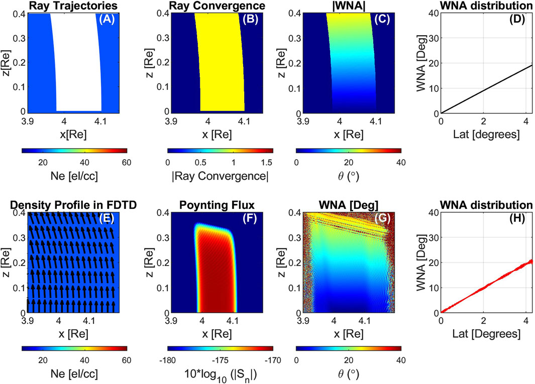
Figure 2. Simulation of non-ducted whistler mode wave propagation in homogeneous density (i) Ray tracing model (top panels A–D); (ii) FDTD model (bottom panels E–H).

The ray tracing model for the homogeneous case consists of 10,000 rays initiated with a wave normal angle of zero degrees shown in white lines (Figure 2A). As there are no ducts or plasma irregularities present, all the rays act as “free rays” following trajectories affected only by geomagnetic curvature. The ray convergence parameter is shown in Figure 2B. In this simulation, the distance between the main rays is 76.4 m and the distance between the main rays and their twin rays is 20 m. As these rays propagate away from the source, we can calculate the ray convergence between the twins. It is expected from ray tracing theory that in the absence of any guiding structures, the waves will have increasing wave normal angles with higher latitude. In our ray tracing code, we can recreate the relation between WNA distribution and increasing latitude. The rays are launched at the equator with a wave normal angle of zero degrees. As these rays travel to higher latitude, the wave normal angle increases due to geomagnetic curvature (Figure 2C). A plot of WNA distribution as a function of latitude is also presented in Figure 2D, for a single ray that starts from x = 4.05 Re. The WNA behavior as a function of latitude for the remaining 10,000 rays in this homogeneous medium scenario is similar. It shows that in our ray tracing simulations, we can trace a ray at L = 4.05 from the equatorial source point to the end of the simulation, and the result aligns with the expected ray tracing theory.

The FDTD model results shown in the bottom panels of Figures 2E–H can be compared with those of the ray tracing simulation in Figures 2A–D. A challenge in full wave simulations is ideal non-reflecting boundary conditions. Here, the simulation is stopped before the waves reach the boundary of the simulation space such that reflected waves do not contaminate the simulation. For this reason, the WNA in Figure 2G shows high values near the upper boundary of the simulation. The direction of the background magnetic field is shown with arrows in Figure 2E. The energy flow of the waves is initially parallel to the background magnetic field and can be calculated via the Poynting flux as displayed in Figure 2F. The Poynting flux shows good agreement in spatial extent and curvature with the ray convergence calculation using the ray tracing model. The average WNA distribution is also calculated as a function of latitude using the FDTD model (Figure 2H) along the ray trajectory of the single ray that starts from x = 4.05 Re that was shown in Figure 2D. Since the FDTD provides a full wave simulation, we can utilize the x and z-positions from ray tracing to extract the WNA values at those specific positions. The FDTD model confirms the increase in WNA with increasing latitude that is seen in the ray tracing simulation results.

4 Simulation results for wave propagation in the presence of ducts

To compare the simulation results with spacecraft data, we examine a time interval from 12:00 to 14:00 UT on 28 May 2017, from the Van Allen Probes A (VAPA, operated from 2012 to 2019) measurements shown in Figure 1A. VAPA was located at L = 4.5–4.6, at magnetic latitude $\lambda$ = -10.6^o. The sharp density enhancement region was from 25 to 30 electron/cm³ to 200–250 electron/cm³ with a spatial scale structure of ∼300–350 km across the background magnetic field direction. The simulation step calculation is dependent on the plasma frequency ($f_p$) which in turn relies on the density profile. To ensure a computable simulation, we reduced the density by a factor of 4 with a maximum density of 50 electron/cm³. The duct-like structure affected the whistler wave, observed in the 0.2–2 kHz frequency range. The data demonstrates enhanced activity inside the structure and suggests that the whistler wave was trapped inside the positive density duct. The wave spectral power in the vicinity of the structure is also affected by the duct: the clear “shadow effect” is seen in the wave power just after the crossing the structure at higher L-shells. This observational event is simulated using ray tracing and full wave models that include geomagnetic curvature in the sub-sections below.

4.1 Ray tracing results

Observational evidence from spacecraft suggests the existence of significant field aligned density irregularities in the vicinity of the equator. To simulate such scenarios, we create field-aligned ducts as shown in Figure 3A, which capture the shape of the density fluctuations and the net change in wave amplitude as shown in Figure 1A. The maximum density region is 50 electrons/cm³ and the wave frequency is 300 Hz (Figure 3A). The rays are launched from the equatorial plane ($\left.z=0\right)$ with a WNA of zero degrees with the source covering approximately $4.76<L<4.85$.

Figure 3

Figure 3. Simulation results of Ray Tracing. (A) Density irregularity region as ray path (B) Ray convergence (C) WNA of rays in degrees. The black dashed line in each plot shows the linecut at $\lambda =3°latitude$.

Here, we initiate 10,000 rays that are initially field aligned to create a large equatorial source region. Figures 3B,C show the ray convergence and WNA distribution. In Figure 3B, the original distance between the main rays and their twin ray is 10 m at z = 0. It is observable that most of the rays are guided to propagate in the field aligned direction inside the duct and there is a shadow region outside the duct near the higher x-coordinate boundary region of the duct. Within the shadow region, less rays propagate.

To characterize the guided and unguided trajectories in more detail, we simulated 20 rays that cover both the inside and outside of the duct. In the presence of ducts, the propagating rays start from the source with WNA, $\theta =0°$ and follow a propagation path along the duct. These rays are categorized into four types in Figure 4, depending on their diverse trajectories and interaction with the duct in different ways.

Figure 4

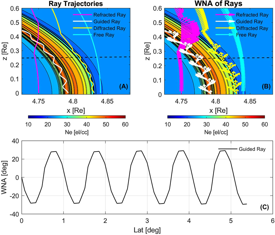
Figure 4. Simulation of four different rays. (A) Ray path trajectory (B) WNA trajectory of rays (C) WNA trajectory of rays, arrows indicate relative wave normal vector. The black dashed line in each plot shows the linecut at $\lambda =3°latitude$.

The four categories of rays are as follows and representative rays of each category are shown with different colors in Figures 4A,B. The Figures 4A,B illustrate the corresponding ray paths for the four types of rays as they propagate along the inhomogeneous density profile of the duct, along with their associated changes in WNA. The arrows in Figure 4B, show the local direction of the wave normal and the arrow length is proportional to the refractive index magnitude.

1. Refracted Ray (magenta): These rays start from the lower edge of the duct. Initially, they do not encounter the duct. But as the waves propagate to higher latitude, they impinge on the lower edge of the duct. This leads to refraction as the waves go across the duct and escape at the other side.

2. Guided/Ducted Rays (white): These rays are launched inside the duct. They exhibit a snaking trajectory staying confined inside the duct. These rays remain confined for the full simulation time.

3. Diffracted Rays (yellow): These rays start at the top edge of the duct. They propagate along the edge and eventually escape the duct.

4. Free rays (cyan): These rays start at the top edge of the duct. These rays do not interact or collide onto the duct at any point in the simulation. They propagate in the smooth background plasma behaving as the rays in a non-ducted case.

In Figure 4C, we show the WNA distribution for the rays that are guided inside the duct as a function of latitude in the presence of geomagnetic curvature. It is worth noting that these guided rays’ WNA is not strictly close to zero but instead oscillates about zero such that the rays snake around the magnetic field as was postulated by (Smith et al., 1960). Such oscillations between $\pm 30°$ can have ramifications for particle scattering and diffusion calculations where the WNA is a key term. In the presence of geomagnetic curvature, some rays may escape out of the duct. This phenomenon may emerge as leakage of wave energy from the duct.

4.2 Finite difference time domain (FDTD) results

We perform a two-dimensional FDTD simulation driven by a source at the equator with similar parameters used in Section 4.1 for ray tracing. The results of a comprehensive simulation study are shown in Figure 5 with the density profile shown in Figure 5A. Within the duct region, the density profile exhibits small-scale density irregularities such that there are smaller ducts within a larger duct.

Figure 5

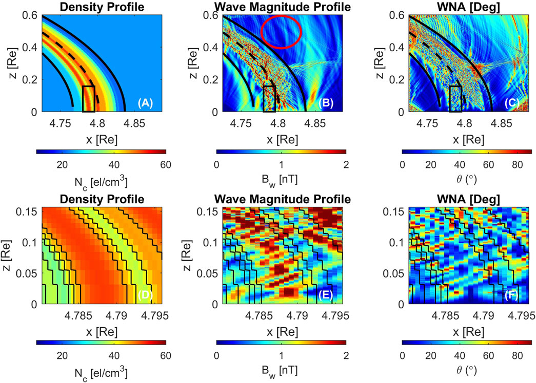
Figure 5. Full wave simulation of the duct using FDTD. (A) density profile (B) wave magnitude profile (C) WNA (D), (E,F) show the region of ∼100 km.

For the FDTD simulation, the wave frequency is also set at 300 Hz, which is 0.04 times the gyrofrequency and in the center of the band of the observed whistler waves. A circularly polarized source is initiated at the magnetic equator and is uniform across all L-shells of interest. This type of source represents a large equatorial source of hiss type waves.

The density variation in Figure 5A displays the magnetospheric duct region throughout the simulation space. To further demonstrate the effect of ducting under a small region of 100 km, a black rectangle area is displayed in the top panels of Figure 5. The lower panels of Figures 5D–F show the wave parameters within this rectangle.

In Figure 5B, the wave magnitude ($B_{w }$ [nT]) is plotted. As the whistler waves that are being guided inside the duct propagate away from the source, the spatial structure of the wave magnitude is influenced by the fluctuation of cold plasma density. The waves that are trapped inside the duct retain a propagation direction parallel to the magnetic field lines resulting from a guiding effect. The guiding of the waves causes enhancement in wave amplitude. The wave magnitude profile for guided waves from the full wave model shows qualitative similarity to the ray convergence profile shown in Figure 3B. The average wave magnitude decreases as the waves go further away from the source, and the propagating waves become oblique. Due to the multiple reflections and complex guiding of the wave inside the duct, there is sub wavelength modulation that occurs within the small structures of the duct. There is a visible pattern of interference causing the rise and fall of wave amplitude and WNA. The fluctuations in amplitude are visible even near the source. It is worth noting that although the electric field excitation at the source is uniform, the density inhomogeneity leads to the formation of a non-uniform planar source. Hence, the density profile structure of the duct causes immediate distortion of the planar wavefront across the duct upon initiation of propagation.

During the guided propagation, the average WNA stays close to zero. For the few waves that escape or propagate outside the duct, the WNA increases with increasing latitude. It is worth noting that such constructive/destructive interference that is a function of wave phase cannot be obtained from the raytracing model. The raw results from FDTD exhibit all the small-scale features for the waves that are spread throughout the simulation space.

In panels (D-F) of Figure 5, the black rectangle region shows the density profile inside the duct that explicitly exhibits small-scale features, or “mini-ducts”, inside the actual large duct. Inside the mini-ducts, the waves show similar features, i.e., periodic change in wave magnitude and WNA.

To compare the model results-directly to observations, we consider a hypothetical satellite to be passing through in the x direction approximately at (i) z₀ = 0, at equator; (ii) z₁ = 172 km; (iii) z₂ = 1601.7 km or $3°$ latitude line cut.

The position of the hypothetical satellite is chosen such that we can study the relationship between the power density ($S_n$) and WNA as the waves propagate along the magnetospheric duct. The different line cuts of interest are shown in white in Figures 6A–C. The power density profile in Figure 6B shows the results after the time average filter has been implemented. In Figures 6D–F, the relationship between the time averaged power density (Sn[dB]) and WNA(θ[degrees]) with density (Ne[el/cc]) is presented. Figure 6D shows the results from the equator where the source is initiated with WNA, θ = 0°. Therefore, the waves are completely field aligned. In Figure 6E, the line cut is at 172 km which is still relatively close to the equator. For this reason, the WNA and power density show similar variations versus L-shell. The average WNA is still low (<30°) for the most part, but there are singular points where the WNA achieves highly oblique values of up to 60°. Figure 6F shows a line cut at 3° latitude where the WNA inside the magnetospheric duct is seen to be increased overall and shows significant peaks of about 85°. Interestingly, the peaks in WNA concur with decreases in the time average power density.

Figure 6

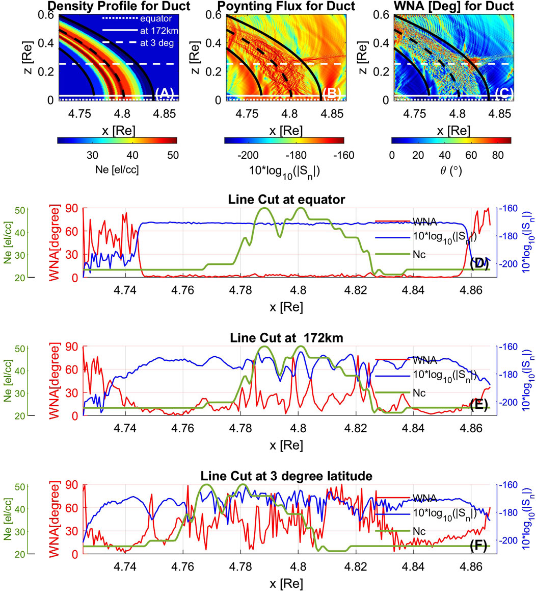
Figure 6. FDTD simulation results for ducted whistler mode wave propagation. (A) Density profile (B) Poynting Flux (C) WNA. At three different latitudinal positions: (D) at the magnetic equator (z₀); (E) 172 km (0.027 R_e) from the equator (z₁); and (F) 1601.7 km (∼3° latitude) from the equator (z₂).

The WNA and power density variations are much richer and more complex in full wave model than those predicted by the raytracing model. The raytracing model showed waves confined in ducts to be either mostly field-aligned or to exhibit the oscillatory ‘snaking’ like behavior (Figure 4C). Both the ray tracing and FDTD models show similarity in leakage at the upper duct boundary due to geomagnetic curvature. Nonetheless, FDTD results show high and somewhat random variations of parameters inside the ducted space with increasing latitude. The higher variation is a result of the constructive/destructive interference enabled by modeling of the wave instantaneous phase. In particular, the fact that the power density decreases coincide with the spikes in the WNA suggest destructive interference at these locations. Moreover, the FDTD model is more sensitive to the small-scale variations that locally distort the planar wavefronts. Another feature that is observed in both the simulation models is the shadowing effect of the ducts (shown in Figure 5B highlighted by the red circle) that is caused by the positioning of the source along the equatorial line and presence of geomagnetic curvature.

5 Discussion and summary

A general problem in investigating whistler mode wave phenomena in the magnetosphere is that in situ observations are extremely sparse. There is therefore a need for accurate models that can predict wave parameters and their evolution in space and time. Here we have deployed two numerical models to simulate whistler mode wave propagation in the presence of cold plasma variations in the background magnetic field and geomagnetic curvature. The raytracing and FDTD models employed here allow us to investigate the effects of propagation without amplification. Likewise, the assumption of a uniform and coherent monochromatic equatorial wave source large over a large range of L-shells is a simplifying assumption that permits honing in on propagation phenomena. Prior studies (Streltsov et al., 2006; Chen et al., 2009) primarily focused on applying either one of the two models individually. After cross-validating the models on the most simplified scenario of whistler mode wave propagation through a homogeneous density environment, we analyzed wave propagation under geomagnetic curvature conditions and field aligned density structures using both models. The unique ducting event observed by Van Allen Probe A provided an opportunity to study the influence of micro-duct structures on whistler mode wave propagation. It should be noted that our models do not take into account cyclotron wave growth that can be important for chorus waves in the equatorial region (Agapitov et al., 2018) nor Landau damping which becomes significant for oblique waves. Whether hiss waves experience growth in the equatorial region or simply propagate into the plasmasphere is less clear.

The raytracing model represents a simplified view of whistler mode wave propagation and tracks the wave normal angle and group velocity of independent wave packets. On the other hand, the FDTD method does a grid-based computation to solve the full set of field values from Maxwell’s equations in a cold plasma fluid. The FDTD model is able to provide Poynting flux directly while the raytracing model permits us to calculate an analogous ray convergence metric. In the case of whistler mode waves propagating in homogeneous cold plasma, both the ray tracing and FDTD model show linear increment of WNA with increasing latitude as waves propagate away from an equatorial source.

For the case of whistler mode wave propagation in the presence of field-aligned density ducts, which was motivated by VAPA EMFISIS observations on 28 May 2017 (Figure 1A), there are some similarities in the predictions of the two models. On the one hand, both the models simulate the propagation structure of whistler mode waves with regions of different wave activity. In the ray tracing results, rays are seen to avoid certain regions along with ducted propagation, leading to areas of low ray convergence. These regions can be interpreted as an indication for reduced wave magnitude (Figure 3B). Similarly, the FDTD simulation also captures regions with low wave magnitude or shadow regions outside the duct as seen in Figure 5B (highlighted by the red circle). These regions closely resemble the area of low wave intensity observed in the VAPA data, indicted with a light blue region in the top panel of Figure 1A. Thus, despite the models differing physical assumptions and computational framework, both models consistently identify the presence of a shadow region which is likely caused by the trapping of the whistler mode waves within the duct and the effects of geomagnetic curvature.

There is also qualitative agreement between ray convergence and full wave power density. The regions where ray paths converge correspond to high wave magnitude and Poynting flux in FDTD simulations. The effects of micro-duct or small-scale ducts are also captured by both these models. At the same time, there are also noticeable differences between the two models. The difference is that the full wave model shows strong effects of constructive/destructive interference behavior. Such interference effects are only prominent in the presence of ducts since the duct structure disrupts the large-scale plane wave behavior. These interferences due to wave interactions can drive the WNA to be locally higher and exhibit higher variation in comparison to the ray tracing model which treats whistler-mode waves purely as rays. Overall, we can conclude that propagation effects alone predict a wider range of instantaneous WNA based on different types of rays propagating along the field-aligned irregularities region. This wider range is in agreement with some past studies. Namely, Harid et al. (2024) show fluctuations of WNA in the range of 0°–20° for ducted waves, and broader statistical studies by Haque et al. (2010) indicate that for parallel-propagating waves, the WNA can vary up to 30°.

Ray tracing theory suggests that a duct must be larger than one wavelength in the transverse direction waves to be confined. Although the observed inhomogeneous density region had at least two regions that are closer to a wavelength, the whistler waves propagated in those regions. This suggests that ray tracing can still produce meaningful results even at the limits of its validity. The minimum limit for the duct regions that can guide the waves is still a matter to be studied.

Another important issue is computation cost. The FDTD and ray tracing simulations were performed by MATLAB software. The two-dimensional FDTD simulation required approximately 6 days to compute the full wave model on a laptop (Core i7-10750H Processor, 32 GB RAM). The ray tracing code took approximately 1 h for computation of the ray path of the initial 10,000 rays in the background magnetic field and calculated the WNA along with the ray convergence in the same device used for FDTD simulation.

These simulation results indicate that the multiple closely spaced density structures in geomagnetic curvature have a significant and complex impact on the wave propagation characteristics. In large-scale ducts, the effects of the spatial profile on wave propagation are not easily predicted from a simple ducted theory, as these structures cannot be treated as independent ducts. The spatial profile of wave distribution for such cases has not been studied extensively in prior research.

Data availability statement

The datasets presented in this study can be found in online repositories. The names of the repository/repositories and accession number(s) can be found in the article/supplementary material.

Author contributions

RK-E-Z: Formal Analysis, Methodology, Software, Visualization, Writing – original draft, Writing – review and editing. VH: Conceptualization, Formal Analysis, Methodology, Software, Supervision, Writing – review and editing. MG: Conceptualization, Formal Analysis, Funding acquisition, Methodology, Supervision, Writing – review and editing. OA: Formal Analysis, Funding acquisition, Investigation, Writing – review and editing. PH: Formal Analysis, Software, Writing – review and editing.

Funding

The author(s) declare that financial support was received for the research and/or publication of this article. This work was supported by the National Science Foundation with Award AGS 2312282 and by NASA with Award 80NSSC19K0264 to University of Colorado Denver. O.V. Agapitov at SSL was supported by NSF grant No. 1914670, NASA’s Living with a Star (LWS) program (contract 80NSSC20K0218), and NASA grants contracts 80NNSC19K0848, 80NSSC22K0433, 80NSSC22K0522, 80NSSC20K0697, and 80NSSC20K0697. R. Khatun-E-Zannat was partially funded by NASA’s Living with a Star (LWS) program (contract 80NSSC20K0218).

Conflict of interest

The authors declare that the research was conducted in the absence of any commercial or financial relationships that could be construed as a potential conflict of interest.

Generative AI statement

The author(s) declare that no Generative AI was used in the creation of this manuscript.

Publisher’s note

All claims expressed in this article are solely those of the authors and do not necessarily represent those of their affiliated organizations, or those of the publisher, the editors and the reviewers. Any product that may be evaluated in this article, or claim that may be made by its manufacturer, is not guaranteed or endorsed by the publisher.

References

Abel, B., and Thorne, R. M. (1998). Electron scattering loss in Earth’s inner magnetosphere: 2. Sensitivity to model parameters. J. Geophys. Res. Space Phys. 103, 2397–2407. doi:10.1029/97JA02920

CrossRef Full Text | Google Scholar

Agapitov, O., Krasnoselskikh, V., Dudok de Wit, T., Khotyaintsev, Y., Pickett, J. S., Santolík, O., et al. (2011a). Multispacecraft observations of chorus emissions as a tool for the plasma density fluctuations’ remote sensing. J. Geophys. Res. Space Phys. 116. doi:10.1029/2011JA016540

CrossRef Full Text | Google Scholar

Agapitov, O., Krasnoselskikh, V., Khotyaintsev, Y. V., and Rolland, G. (2011b). A statistical study of the propagation characteristics of whistler waves observed by cluster. Geophys. Res. Lett. 38. doi:10.1029/2011GL049597

CrossRef Full Text | Google Scholar

Agapitov, O., Artemyev, A., Krasnoselskikh, V., Khotyaintsev, Y. V., Mourenas, D., Breuillard, H., et al. (2013). Statistics of whistler mode waves in the outer radiation belt: cluster STAFF-SA measurements. J. Geophys. Res. Space Phys. 118, 3407–3420. doi:10.1002/jgra.50312

CrossRef Full Text | Google Scholar

Agapitov, O. V., Artemyev, A. V., Mourenas, D., Mozer, F. S., and Krasnoselskikh, V. (2015). Empirical model of lower band chorus wave distribution in the outer radiation belt. J. Geophys. Res. Space Phys. 120 (10), 425–442. doi:10.1002/2015JA021829

CrossRef Full Text | Google Scholar

Agapitov, O., Mourenas, D., Artemyev, A., Mozer, F. S., Bonnell, J. W., Angelopoulos, V., et al. (2018). Spatial extent and temporal correlation of chorus and hiss: statistical results from multipoint THEMIS observations. J. Geophys. Res. Space Phys. 123, 8317–8330. doi:10.1029/2018JA025725

CrossRef Full Text | Google Scholar

Bortnik, J., and Thorne, R. M. (2007). The dual role of ELF/VLF chorus waves in the acceleration and precipitation of radiation belt electrons. J. Atmos. Solar-Terrestrial Phys. 69, 378–386. doi:10.1016/j.jastp.2006.05.030

CrossRef Full Text | Google Scholar

Bortnik, J., Inan, U. S., and Bell, T. F. (2003). Energy distribution and lifetime of magnetospherically reflecting whistlers in the plasmasphere. J. Geophys. Res. Space Phys. 108. doi:10.1029/2002JA009316

CrossRef Full Text | Google Scholar

Bortnik, J., Thorne, R., and Meredith, N. (2008). The unexpected origin of plasmaspheric hiss from discrete chorus emissions. Nature 452, 62–66. doi:10.1038/nature06741

PubMed Abstract | CrossRef Full Text | Google Scholar

Bortnik, J., Chen, L., Li, W., Thorne, R. M., and Horne, R. B. (2011). Modeling the evolution of chorus waves into plasmaspheric hiss. J. Geophys. Res. Space Phys. 116. doi:10.1029/2011JA016499

CrossRef Full Text | Google Scholar

Breuillard, H., Zaliznyak, Y., Krasnoselskikh, V., Agapitov, O., Artemyev, A., and Rolland, G. (2012). Chorus wave-normal statistics in the Earth’s radiation belts from ray tracing technique. Ann. Geophys. 30, 1223–1233. doi:10.5194/angeo-30-1223-2012

CrossRef Full Text | Google Scholar

Chen, L., Bortnik, J., Thorne, R. M., Horne, R. B., and Jordanova, V. K. (2009). Three-dimensional ray tracing of VLF waves in a magnetospheric environment containing a plasmaspheric plume. Geophys. Res. Lett. 36. doi:10.1029/2009GL040451

CrossRef Full Text | Google Scholar

Chen, L., Thorne, R. M., Bortnik, J., Li, W., Horne, R. B., Reeves, G. D., et al. (2014). Generation of unusually low frequency plasmaspheric hiss. Geophys. Res. Lett. 41, 5702–5709. doi:10.1002/2014GL060628

CrossRef Full Text | Google Scholar

Chen, R., Gao, X., Lu, Q., Chen, L., Tsurutani, B. T., Li, W., et al. (2021). In situ observations of whistler-mode chorus waves guided by density ducts. J. Geophys. Res. Space Phys. 126, e2020JA028814. doi:10.1029/2020JA028814

CrossRef Full Text | Google Scholar

Gołkowski, M., and Inan, U. S. (2008). Multistation observations of ELF/VLF whistler mode chorus. J. Geophys. Res. Space Phys. 113. doi:10.1029/2007JA012977

CrossRef Full Text | Google Scholar

Hanzelka, M., and Santolík, O. (2019). Effects of ducting on whistler mode chorus or exohiss in the outer radiation belt. Geophys. Res. Lett. 46, 5735–5745. doi:10.1029/2019GL083115

CrossRef Full Text | Google Scholar

Hanzelka, M., and Santolík, O. (2022). Effects of field-aligned cold plasma density filaments on the fine structure of chorus. Geophys. Res. Lett. 49, e2022GL101654. doi:10.1029/2022GL101654

CrossRef Full Text | Google Scholar

Haque, N., Spasojevic, M., Santolík, O., and Inan, U. S. (2010). Wave normal angles of magnetospheric chorus emissions observed on the polar spacecraft. J. Geophys. Res. Space Phys. 115. doi:10.1029/2009JA014717

CrossRef Full Text | Google Scholar

Harid, V., Agapitov, O., Khatun-E-Zannat, R., Gołkowski, M., and Hosseini, P. (2024). Complex whistler-mode wave features created by a high density plasma duct in the magnetosphere. J. Geophys. Res. Space Phys. 129, e2023JA032047. doi:10.1029/2023JA032047

CrossRef Full Text | Google Scholar

Horne, R. B. (1989). Path-integrated growth of electrostatic waves: the generation of terrestrial myriametric radiation. J. Geophys. Res. Space Phys. 94, 8895–8909. doi:10.1029/JA094iA07p08895

CrossRef Full Text | Google Scholar

Hosseini, P., Golkowski, M., Agapitov, O. V., and Harid, V. (2020). Full wave modeling of small scale plasma irregularities and effects on whistler mode chorus propagation, SM025–SM028.

Google Scholar

Hosseini, P., Agapitov, O., Harid, V., and Gołkowski, M. (2021). Evidence of small scale plasma irregularity effects on whistler mode chorus propagation. Geophys. Res. Lett. 48, e2021GL092850. doi:10.1029/2021GL092850

CrossRef Full Text | Google Scholar

Inan, U. S., and Bell, T. F. (1977). The plasmapause as a VLF wave guide. J. Geophys. Res. (1896-1977) 82, 2819–2827. doi:10.1029/JA082i019p02819

CrossRef Full Text | Google Scholar

Inan, U. S., Chang, H. C., Helliwell, R. A., Imhof, W. L., Reagan, J. B., and Walt, M. (1985). Precipitation of radiation belt electrons by man-made waves: a comparison between theory and measurement. J. Geophys. Res. Space Phys. 90, 359–369. doi:10.1029/JA090iA01p00359

CrossRef Full Text | Google Scholar

Katoh, Y. (2014). A simulation study of the propagation of whistler-mode chorus in the Earth’s inner magnetosphere. Earth, Planets Space 66, 6–12. doi:10.1186/1880-5981-66-6

CrossRef Full Text | Google Scholar

Ke, Y., Chen, L., Gao, X., Lu, Q., Wang, X., Chen, R., et al. (2021). Whistler-mode waves trapped by density irregularities in the earth’s magnetosphere. Geophys. Res. Lett. 48, e2020GL092305. doi:10.1029/2020GL092305

CrossRef Full Text | Google Scholar

Kimura, I. (1966). Effects of ions on whistler-mode ray tracing. Radio Sci. 1, 269–284. doi:10.1002/rds196613269

CrossRef Full Text | Google Scholar

Maxworth, A., and Golkowski, M. (2017). “Warm plasma raytracing of whistler mode waves in the Earth’s magnetosphere,” in 2017 United States national committee of URSI national radio science meeting (USNC-URSI NRSM), 1–2. doi:10.1109/USNC-URSI-NRSM.2017.7878320

CrossRef Full Text | Google Scholar

Maxworth, A. S., Gołkowski, M., Malaspina, D. M., and Jaynes, A. N. (2020). Raytracing study of source regions of whistler mode wave power distribution relative to the plasmapause. J. Geophys. Res. Space Phys. 125, e2019JA027154. doi:10.1029/2019JA027154

CrossRef Full Text | Google Scholar

Meredith, N. P., Horne, R. B., Clilverd, M. A., Horsfall, D., Thorne, R. M., and Anderson, R. R. (2006). Origins of plasmaspheric hiss. J. Geophys. Res. Space Phys. 111. doi:10.1029/2006JA011707

CrossRef Full Text | Google Scholar

Pasmanik, D. L., and Demekhov, A. G. (2017). Peculiarities of VLF wave propagation in the Earth’s magnetosphere in the presence of artificial large-scale inhomogeneity. J. Geophys. Res. Space Phys. 122, 8124–8135. doi:10.1002/2017JA024118

CrossRef Full Text | Google Scholar

Pasmanik, D. L., and Demekhov, A. G. (2020). On the influence of propagation properties of whistler-mode waves in the Earth’s magnetosphere on their cyclotron amplification. Radiophys. Quantum Electron. 63, 241–256. doi:10.1007/s11141-021-10049-z

CrossRef Full Text | Google Scholar

Shklyar, D. R. (2005). Key problems in numerical simulation of spectrograms related to emissions caused by lightning stroke. Geomagnetism Aeronomy 45, 474–487.

Google Scholar

Shklyar, D. R., Chum, J., and Jiříček, F. (2004). Characteristic properties of nu whistlers as inferred from observations and numerical modelling. Germany: Copernicus Publications Göttingen.

Google Scholar

Smith, R. L., Helliwell, R. A., and Yabroff, I. W. (1960). A theory of trapping of whistlers in field-aligned columns of enhanced ionization. J. Geophys. Res. (1896-1977) 65, 815–823. doi:10.1029/JZ065i003p00815

CrossRef Full Text | Google Scholar

Sonwalkar, V. S., Inan, U. S., Bell, T. F., Helliwell, R. A., Chmyrev, V. M., Sobolev, Ya. P., et al. (1994). Simultaneous observations of VLF ground transmitter signals on the DE 1 and COSMOS 1809 satellites: detection of a magnetospheric caustic and a duct. J. Geophys. Res. Space Phys. 99, 17511–17522. doi:10.1029/94JA00866

CrossRef Full Text | Google Scholar

Stix, T. H. (1992). Waves in plasmas. Springer Science and Business Media.

Google Scholar

Streltsov, A. V., Lampe, M., Manheimer, W., Ganguli, G., and Joyce, G. (2006). Whistler propagation in inhomogeneous plasma. J. Geophys. Res. Space Phys. 111. doi:10.1029/2005JA011357

CrossRef Full Text | Google Scholar

Streltsov, A. V., Lampe, M., and Ganguli, G. (2007). Whistler propagation in nonsymmetrical density channels. J. Geophys. Res. Space Phys. 112. doi:10.1029/2006JA012093

CrossRef Full Text | Google Scholar

Williams, D. D., and Streltsov, A. V. (2021). Determining parameters of whistler waves trapped in high-density ducts. J. Geophys. Res. Space Phys. 126, e2021JA029228. doi:10.1029/2021JA029228

CrossRef Full Text | Google Scholar

Yearby, K. H., Balikhin, M. A., Khotyaintsev, Y. V., Walker, S. N., Krasnoselskikh, V. V., Alleyne, H. S. C. K., et al. (2011). Ducted propagation of chorus waves: cluster observations. Ann. Geophys. 29, 1629–1634. doi:10.5194/angeo-29-1629-2011

CrossRef Full Text | Google Scholar

Yee, K. (1966). Numerical solution of initial boundary value problems involving maxwell’s equations in isotropic media. IEEE Trans. Antennas Propag. 14, 302–307. doi:10.1109/TAP.1966.1138693

CrossRef Full Text | Google Scholar

Zhang, S., Rae, I. J., Liu, K., Watt, C. E. J., Shi, Q., Tian, A., et al. (2024). Effects of plasma density on the spatial and temporal scale sizes of plasmaspheric hiss. J. Geophys. Res. Space Phys. 129, e2023JA031955. doi:10.1029/2023JA031955

CrossRef Full Text | Google Scholar

Zudin, I.Yu., Zaboronkova, T. M., Gushchin, M. E., Aidakina, N. A., Korobkov, S. V., and Krafft, C. (2019). Whistler waves’ propagation in plasmas with systems of small-scale density irregularities: numerical simulations and theory. J. Geophys. Res. Space Phys. 124, 4739–4760. doi:10.1029/2019JA026637

CrossRef Full Text | Google Scholar