Investigation of phase and power fluctuation events using Rytov method and the forward propagation model

Ionospheric density irregularities cause fluctuations in transionospheric satellite signals, known as “scintillation”. While scintillation degrades the performance of navigation satellites, such as the Global Positioning System (GPS), it also serves as a diagnostic tool for studying the underlying plasma processes. In this study, we characterize high-latitude ionospheric structuring and its impact on radio signals using a 3D propagation model, the “Satellite-beacon Ionospheric-scintillation Global Model of the upper Atmosphere” (SIGMA), in conjunction with GPS observations and an analytical model. Establishing a modeling framework for defining the irregularity parameters, including spatial extent, spectral index, axial ratios, density fluctuations, layer height, drift velocity, and thickness, is essential for providing insights into scintillation modeling. We use the Rytov method, a well-known analytical 2D model for estimating irregularity parameters from observed log-power and phase spectra, which is particularly useful in the absence of auxiliary observations. Observations from GPS array receivers in Poker Flat, Alaska, are used to examine the simultaneous occurrence of phase and power fluctuations. These occurrences are rare, as only a few such events were detected in observations from 2014 to 2019. These reveal both large-scale, refractive fluctuations and smaller-scale, diffractive features embedded within them, highlighting the multiscale nature of plasma structuring. Initializing SIGMA with Rytov-derived parameters shows a good agreement between the simulated and observed power spectral densities, with goodness-of-fit metric $({\chi }^{\prime })$ close to 1. This is observed with power fluctuations, particularly when shorter temporal segments are used for the inversion. A spectral break within the diffractive regime suggests the presence of multiscale structuring. Overall, our findings support the concept that turbulent energy cascading from large-scale structures, likely driven by gradient-drift and/or Kelvin–Helmholtz instabilities, plays a crucial role in generating scintillation-inducing irregularities.

1 Introduction

Ionospheric scintillation refers to rapid fluctuations in the power and phase of radio signals as they propagate through the Earth’s ionosphere. These fluctuations are caused by electron density irregularities that act as a random medium. Studying these irregularities provides critical insight into the processes that cause scintillation, allowing us to better model and forecast these phenomena. When radio waves from Global Navigation Satellite Systems (GNSS), such as the Global Positioning System (GPS), encounter ionospheric irregularities, they undergo phase fluctuations (due to changes in refractive index) and power fluctuations (due to constructive and destructive interference patterns), particularly under weak-scatter, forward-scatter conditions (Yeh and Liu, 1982). These effects can significantly degrade the performance of the GNSS, especially under geomagnetically disturbed conditions (Basu et al., 1999; Kintner et al., 2007).

In the auroral ionosphere, electron density irregularities are believed to originate and develop in response to various sources of energy input, including influences from the magnetosphere, energetic precipitation, and plasma instabilities such as gradient-drift instability (GDI), and Kelvin-Helmholtz instability (KHI) (Kintner and Seyler, 1985). Large-scale plasma density patch can enter through the cusp region and transits through the polar cap into the auroral zone. During this transit, various plasma processes act on them to structure them into different scales (van der Meeren et al., 2014), a process known as cascading. In turbulent energy cascading, energy injected at larger spatial scales (the outer scale), is progressively transferred through turbulent mixing to smaller scales until it reaches the smallest scales/dissipation scales (Kintner and Seyler, 1985). The region between the outer scale and dissipation scale is known as the inertial sub-range, where turbulent mixing redistributes energy across scales. As a result, the spectrum of irregularities within this range may differ from the original energy injection scale. Instability-related irregularity formation mechanisms, such as GDI or KHI, act to structure the plasma at F-region altitudes (Carlson et al., 2007) while E-region structures can be formed by particle precipitation and ionization (Enengl et al., 2024). As these density structures evolve into a spectrum of spatial scales (inertial sub-range), they begin to perturb transionospheric radio signals through diffraction and refraction. Foundational theories of wave propagation in random media, such as those developed by Tatarski (2016), Ishimaru (1978); Rino (1979), and Yeh and Liu (1982), provide the analytical framework for interpreting how these multiscale irregularities influence signal propagation.

To understand the scintillation data, we employ power spectral density (PSD) analysis, a common technique used to identify different scale sizes present in scintillation-inducing irregularities, as well as to probe underlying plasma turbulence and instability dynamics (Yeh and Liu, 1982; Tsunoda, 1988). PSD analysis forms the basis of the phase screen theory developed by Rino (1979), which models ionospheric scintillation by characterizing the irregularity spectrum as a power-law distribution. This theoretical framework relates the spectral slope to both the intensity and scale distribution of electron density irregularities, thereby distinguishing between refractive and diffractive effects (Rino, 2011). Phase fluctuations can arise from refractive bending in regions of large-scale spatial gradients or rapid phase shifts along the signal path. Power fluctuations typically result from diffractive effects caused by irregularities on the order of Fresnel scales $(\sim \sqrt{\lambda z})$, which depend on signal wavelength $(\lambda )$ and the distance of the irregularity layer from the receiver $(z)$ (Yeh and Liu, 1982). Theoretical developments of double-slope spectra indicate the diagnosis of plasma environments where both refractive bending and diffractive stochastic processes coexist (Basu et al., 1983; Wernik et al., 2003; Rino, 2011), and the transition in spectral slopes links to turbulent energy cascading (Kintner et al., 2007). Small-scale irregularities dominate diffractive/stochastic effects, whereas larger-scale irregularities are associated with refractive/deterministic effects (Rufenach, 1975; Rino, 1979; Bhattacharyya et al., 2000; De Franceschi et al., 2019; Ghobadi et al., 2020).

Despite these theoretical foundations, observational evidence directly connecting turbulent energy cascading to scintillation-inducing irregularities at high latitudes is still limited. In particular, events with simultaneous phase and power fluctuations are uncommon, and methods for extracting irregularity parameters from observed fluctuation spectra in such events remain limited.

The methodology of this study combines the Rytov analytical approach with the forward propagation model, “Satellite-beacon Ionospheric scintillation Global Model of the upper Atmosphere” (SIGMA) (Deshpande et al., 2014). We begin by identifying the simultaneous occurrence of power and phase fluctuations with continuous fluctuations of at least 30 s, along with auxiliary data from instruments such as the Poker Flat Incoherent Scatter Radar (PFISR). Next, we apply the Rytov method (Datta-Barua et al., 2020), a 2D analytical technique, to estimate the irregularity parameters using spectra of observed power and phase fluctuations. These Rytov-derived parameters serve as input to a numerical inverse modeling framework using SIGMA (Deshpande et al., 2016), which performs numerical inverse analysis by refining parameter estimates through comparisons between simulated and observed power spectral densities. The irregularity parameters retrieved through this combined approach include drift speed $(|v_d|)$, drift direction $(\angle v_d)$, RMS electron density fluctuations $(\mathrm{\Delta }{N}_e)$, spectral index of electron density irregularities (SpInd), as well as the height $(z)$ and thickness $(L)$ of the irregularity layer.

SIGMA can be operated in multiple modes depending on the availability of observational data. For example, Vaggu et al. (2023) heavily relied on incoherent scatter radar (ISR) data throughout their analysis, whereas Vaggu et al. (2024) majorly utilized all-sky camera observations to initiate their modeling runs. In the absence of such auxiliary datasets, SIGMA is capable of functioning as a standalone forward model by relying on assumed input conditions. However, when a cluster of GNSS receivers is available and records simultaneous phase and power fluctuations, a more data-driven inverse modeling approach becomes viable. In such cases, the Rytov method can be applied to the observed fluctuation spectra to estimate irregularity parameters. These Rytov-derived estimates can then be used to initialize SIGMA, allowing the simulated power spectral densities (PSDs) to be directly compared with observations for parameter optimization and physical interpretation.

The motivation for this work lies in understanding how turbulent energy cascading in the high-latitude ionosphere gives rise to scintillation-inducing irregularities. While scintillation is widely recognized as a manifestation of plasma structuring, the observational link between multiscale cascading processes and irregularity formation remains to be explored. As scintillation measurements are sensitive to irregularity scales ranging from $\sim 100$ m to $\sim 100$ km, they provide a powerful means of probing the inertial sub-range where cascading transfers energy from large-scale drivers to small-scale irregularities. Observational studies in high-latitude regions show that phase scintillations occur far more frequently than amplitude scintillations (Aaron, 1982; Jiao et al., 2013), while simultaneous phase and amplitude scintillation remains comparatively rare. A multi-year survey from $2014--2019$ by Datta-Barua et al. (2021) reported only a few events exhibited simultaneous phase and amplitude scintillation. Leveraging these measurements offers a unique opportunity to observationally resolve the multiscale cascade of energy and to examine how plasma irregularities evolve from their source mechanisms to the scales that directly impact satellite signals.

A key challenge in this study is identifying high-latitude scintillation events that exhibit simultaneous phase and power fluctuations, as such occurrences are relatively rare. In addition, fitting the PSD of observed and simulated power fluctuations becomes difficult as amplitude scintillation typically occurs in short bursts of only a few $(\sim 5--10)$ seconds. Even with high-rate (50 Hz) sampling, such short intervals limit spectral resolution and reduce the statistical reliability of the PSD estimate. To investigate these events, we apply the Rytov method to derive irregularity parameters from scintillation spectra and use these estimates to initialize the SIGMA inverse framework. Using this approach, we compare the simulated and observed spectra to assess the ionospheric conditions and investigate these events to examine the role of turbulent energy cascading in multiscale plasma structuring.

2 Data and methodology

Scintillation Auroral GPS Array (SAGA) is an array of high-rate GNSS receivers established at the Poker Flat Research Range (PFRR), Alaska (Datta-Barua et al., 2015). The array consists of six GPS receivers, each providing 100 Hz power and phase measurements for satellites tracked at the L1 C/A (1575.42 MHz) and L2C (1227.60 MHz) frequencies. For this study, only L1 data are utilized. We analyze high-rate time series data from SAGA that have been detrended and filtered following the procedures recommended by Deshpande et al. (2012). While several filtering techniques exist to determine the cut-off frequency to separate refractive and diffractive components (Ghobadi et al., 2020), we adopt a 0.1 Hz high-pass filter cutoff that allows us to focus on phase and power fluctuations induced by ionospheric structures, regardless of whether they are responsible for refractive and/or diffractive effects. The 0.1 Hz high-pass filter cutoff separates low-frequency variations due to satellite motion and receiver effects. This choice is also consistent with Van Dierendonck et al. (1993), who applied a sixth-order Butterworth high-pass filter with a 0.1 Hz cutoff to separate scintillation-induced rapid fluctuations from low-frequency signal components in GNSS C/A code receivers.

2.1 Phase and power fluctuation events

We focus on events that exhibit simultaneous phase and power fluctuations. The selected events for this study are: 1) 5 August 2014 at 12:20:13 UTC, and 2) 8 December 2013 at 03:43:55 UTC, (hereafter referred to as Case 1 and Case 2, shown in Figure 1. These observations are taken from multiple SAGA receivers available during the scintillation interval (e.g., IIT-1, IIT-15, IIT-16, etc.). IIT-16 of Case 1 and IIT-1 of Case 2 data are used for SIGMA analysis. One of the primary challenges in this study is identifying events that exhibit both phase and power fluctuations (more events are shown in Section 3). Such events are relatively rare at high latitudes, where scintillation is typically dominated by phase-only fluctuations (Aaron, 1982), especially as determined by low-rate scintillation (Sreenivash et al., 2020). The simultaneous phase and power fluctuations observed by at least three SAGA receivers are required for the Rytov analysis, which is discussed later in this section.

Figure 1

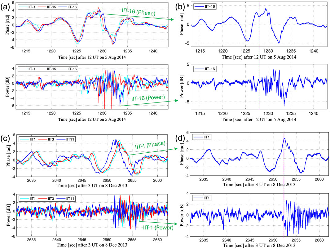
Figure 1. The phase and power fluctuations recorded by SAGA receivers on 5 August 2014 and 8 December 2013. Panels (a,c) data recorded at multiple SAGA IIT receivers. Panels (b,d) focus on IIT-16 and IIT-1 respectively. The magenta dashed line highlights the onset of high-frequency components within the signal phase that coincide with intense power fluctuations.

2.2 Unique observations of the identified events

As mentioned previously, these events are rare because they exhibit both strong power and phase fluctuations. These events are considered rare because, over nearly half a solar cycle $(2014--2019)$, analysis of SAGA $100$s scintillation index data identified only $\sim 30$ amplitude scintillation events, the majority of which occurred during 2014. Of these, only a very few exhibited simultaneous phase and amplitude scintillation recorded across multiple SAGA receivers (Sreenivash et al., 2020; Datta-Barua et al., 2021). By fitting the SIGMA simulated time series of power and phase with the observations, we can analyze the underlying ionospheric conditions and irregularity scale sizes responsible for these fluctuations. Strong power fluctuations are happening for a short period of time in both cases. In Case 1 (Figures 1a,b), the phase fluctuations are observed over the entire scintillation interval, whereas the power fluctuations are observed in the last 15-s interval. During the first 15 s, the phase fluctuations show only long-period variations with no evident high-frequency components (short-period variations) embedded on top of them. In contrast, the last 15 s display long-period fluctuations superimposed on high-frequency, short-period fluctuations. These short-period variations could indicate diffractive effects, which often manifest as fluctuations in signal power. Diffraction typically occurs when irregularities have structures close to or smaller than the Fresnel scale sizes. This becomes particularly important when performing spectral analysis, as discussed in Section 3.2. A similar trend can be observed in Case 2 and other similar cases, as shown in Section 3.4.

Although the occurrence of simultaneous phase and amplitude scintillation is observationally rare, the spectral characteristics exhibited by the modeled events, such as dual-slope power law behavior, spectral breaks near Fresnel scales, and slope values, are not unique and have been reported in many high-latitude studies (Spicher et al., 2014; Carrano and Rino, 2016; McCaffrey and Jayachandran, 2017; Ghobadi et al., 2020).

2.3 Rytov analysis: ratio of log-power spectrum to the phase spectrum

For Rytov analysis, the spectrum of log-power fluctuations Equation 1 and phase fluctuations Equation 2 must be recorded at a minimum of three SAGA receivers. Using at least three receivers ensures robust multi-receiver averaging of spectra and reduces the influence of single-receiver noise. These averaged spectra are then used to compute the ratio of the log-power spectrum to the phase spectrum (Equation 3), which represents theoretical Rytov spectral ratio $(R_f)$, as shown in Equation 4. The Rytov method utilizes the Rytov spectral ratio to infer the properties of ionospheric irregularities, including their layer thickness, height of the ionosphere, drift speed, and drift direction.

For a uniform irregularity layer, the spatial spectra of log-power and phase fluctuations in the horizontal plane are derived by integrating the plasma density fluctuation spectrum $(S_{\mathrm{\Delta }}n)$ along the propagation direction $z$ over the extent of the layer, from $z=0$ to the layer thickness $(L)$ [Taylor, 1975, eq.(31)]

$S_{\chi }=B\left[1-R_f\right]S_{\mathrm{\Delta }n}(1)$

$S_{\varphi }=B\left[1+R_f\right]S_{\mathrm{\Delta }n}(2)$

where $S_{\mathrm{\Delta }n}$ is the spectrum of plasma density variations, and the terms in $B$ (except thickness $L$) are constants for a given signal and geometry as defined by Datta-Barua et al. (2020).

The ratio of the log-power spectrum to the phase spectrum gives a theoretical Rytov spectral ratio $R_f$

$\frac{S_{\chi }}{S_{\varphi }}=\frac{1-R_f}{1+R_f}(3)$

By re-arranging terms, we get

$R_f=\frac{S_{\varphi }-S_{\chi }}{S_{\varphi }+S_{\chi }}(4)$

The corresponding expression for power spectra of phase and log power of the field on the ground is given by [Yeh and Liu, 1982, eq.(3.26)]. It can further be used as a filter for Rytov approximation (forward and weak scatter), expressed as

$R_f=\frac{2k}{k_{\Vert }^{2}L}\sin \left(\frac{k_{\Vert }^{2}L}{2k}\right)\cos \left(\frac{k_{\Vert }^2}{k}\left(z-\frac{L}{2}\right)\right)(5)$

where:

$k=2\pi /\lambda$ is the free-space wavenumber of the GNSS signal, with $\lambda$ the wavelength.

$k_{\Vert }$ is the parallel component of the wave vector (along the propagation/slant path). It is related to the perpendicular component by

$k_{\Vert }=\alpha |k_{\perp }|.$

$k_{\perp }=(k_x,k_y)$ is the wave vector components in the plane perpendicular to the propagation direction of the incoming wave, with magnitude

$|k_{\perp }|=\frac{2\pi f}{v_d},$

where $f$ is the temporal frequency and $v_d$ is the irregularity drift speed.

$•$ $\alpha$ is a geometric factor depending on viewing geometry:

$\alpha =\left[1+{\left(\cos {\theta }_d\cos \varphi +\sin {\theta }_d\sin \varphi \right)}^2\right]{\tan }^2\theta ,$

where ${\theta }_d$ is the drift direction (counter-clockwise from geographic east), $\varphi$ the azimuth angle of propagation, and $\theta$ the zenith angle.

$L$ is the irregularity layer thickness, and $z$ is the height of the ionosphere measured from the ground.

The drift speed $v_d$ and drift direction ${\theta }_d$ are estimated using a multi-receiver cross-correlation technique similar to that of Costa et al. (1988), by utilizing the time lags in correlated signal fluctuations observed across SAGA receivers to infer the horizontal velocity of the drifting ionospheric irregularities. This method assumes that plasma irregularities remain unchanged in structure as they drift across the receiver baseline during the observation interval, an approximation known as the “frozen-in” assumption or Taylor’s hypothesis (Taylor, 1938). Once the drift parameters are extracted, they are treated as fixed inputs in Equation 5, thereby reducing the free parameters to $L$ and $z$. Comparing (4) and (5)

$\frac{S_{\varphi }-S_{\chi }}{S_{\varphi }+S_{\chi }}=\frac{2k}{k_{\Vert }^{2}L}\sin \left(\frac{k_{\Vert }^{2}L}{2k}\right)\cos \left(\frac{k_{\Vert }^2}{k}\left(z-\frac{L}{2}\right)\right)(6)$

In Equation 6, the left-hand side (LHS) is derived from observational data, while the right-hand side (RHS) serves as a model representation that depends on $L$ and $z$. These parameters are estimated by minimizing the difference between the observed and modeled Rytov ratios by using the goodness-of-fit, which is quantified using a mean squared error (MSE) cost function. This approach is similar to the method employed by [Datta-Barua et al., 2020, Eq.(27)], where a cost function is minimized to retrieve the best-fit estimates of $L$ and $z$.

Scintillation measurements obtained along the line-of-sight (LOS) represent a one-dimensional (1D) projection of underlying three-dimensional (3D) electron density irregularities in the ionosphere. By applying a Fourier transform to the fluctuations observed along the LOS, a corresponding 1D spatial spectrum of electron density fluctuations can be derived. Analyzing this spectrum in log-log space can help us identify power-law behavior (such as a Kolmogorov-type slope), which is indicative of scale-dependent structuring. In addition, the 1D spectral index is always two less than the 3D spectral index $({\alpha }_{1D}={\alpha }_{3D}-2)$, as seen in Kolmogorov turbulence, where a 3D index of $11/3$ results in a 1D index of $5/3$. This relationship assumes isotropy and homogeneity in the turbulence (Tatarskii, 1971; Rino, 1979; Yeh and Liu, 1982). Furthermore, the total strength of the electron density fluctuations, $<|\mathrm{\Delta }N{|}^2>$, is obtained by integrating the electron density spectrum over a certain range of spatial wavenumbers, representing contributions from the corresponding spatial scales.

The parameters shown in the Table 1, namely, $|v_d|$, $\angle v_d$, $L_{th}$, $H_{\mathit{iono}}$, $SpInd$, and $N_e$ are derived using the above analysis, and are used as initial input to the SIGMA-inverse analysis.

Table 1

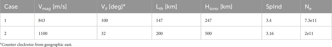
Table 1. Rytov analysis for 5 August 2014 and 8 December 2013 events.

2.4 SIGMA analysis and inversion

SIGMA is a 3D forward radio wave propagation model that simulates the propagation of satellite signals through ionospheric irregularities where the irregularity layers are characterized by the density distribution (Deshpande et al., 2014). SIGMA uses the information of the irregularity parameters, namely, electron number density $(N_e)$, drift speed $(|v_d|)$, drift direction $(\angle v_d)$, spectral index, altitude $(H_{\mathit{iono}})$, no. of layers $(N_l)$, layer thickness (${\text{L}}_{th}$), axial ratio, and outer scale $(l_0)$ and outputs the power and phase time series and its corresponding spectra on the ground. We also perform the SIGMA inversion over a 4D grid space with four design variables ($N_e$, $(|v_d|)$, $\angle v_d$, and spectral index). We assume single values for the other five input parameters, namely, altitude (${\text{H}}_{\mathit{iono}}$), no. of layers (${\text{N}}_l$), layer thickness (${\text{L}}_{th}$), axial ratio (AXR), and outer scale (${\text{l}}_0$) (Deshpande et al., 2016; Vaggu et al., 2023). A high-rate (50 Hz) time series of the simulated complex signal is generated for each parameter set, from which the filtered phase and power time series are derived. The observed power and phase time series from SAGA, as well as the simulated data for the selected event, are then detrended to remove satellite geometry effects and receiver clock errors (Deshpande et al., 2012). Finally, the PSDs of both the observed and simulated time series are extracted to evaluate the PSD fit, as illustrated below.

We use the chi-square fitting test (Press, 2007) to find the best PSD fit of the simulated data to the observed data, as shown in Equation 7. The maximum likelihood estimate of the model parameters is obtained by minimizing the chi-square quantity given by the equation below.

${\chi }^2=\frac{1}{{{\sigma }_y}^2}{\displaystyle \sum _{i=1}^N}{\left({\log }_{10}{Y}_i-{\log }_{10}{X}_i\right)}^2(7)$

where ${\mathrm{l}\mathrm{o}\mathrm{g}}_{10}{Y}_{i}s$ are N number of points on the PSD (dB) of the observed phase, ${\mathrm{l}\mathrm{o}\mathrm{g}}_{10}{X}_{i}s$ are the points on PSD (dB) of the SIGMA phase, and ${{\sigma }_y}^2$ is the variance on the observed PSD after removal of any trends. For a good fit Press (2007), ${\chi }^2$ $\approx$ (N $-$ M) or ${\chi }^{\prime }$ = ${\chi }^2$/(N $-$ M) $\approx$ 1, where the degrees of freedom are represented by (N $-$ M), with M as the total number of design variables to be fitted. In our case, M is 4 as we vary the four design variables to evaluate the chi-square values at each grid point and find the minimal value. The corresponding optimal values of the irregularity parameters, determined for the minimum chi-value, are then extracted to study the ionospheric conditions. The flow chart illustrating the SIGMA process for finding optimal values is shown in Vaggu et al. (2023).

The SIGMA simulations were executed on Embry-Riddle’s Vega high-performance computing (HPC) cluster, which consists of 42 nodes, each equipped with dual AMD EPYC 9654 96-core processors and 1.5 TB of RAM. Simulations were run on a single node utilizing 192 CPU cores. Each forward SIGMA run with a resolution of 100 m required approximately 45–60 min, depending on the irregularity parameters and propagation geometry. The inverse analysis was performed by evaluating the model fit across a four-dimensional parameter grid, with each grid point corresponding to a distinct forward run. Between 16 and 256 forward simulations were conducted per inversion, with each inverse run requiring a total computational time ranging from approximately 12 to 256 h on a single Vega node.

2.5 Solution approach

To derive the irregularity parameters and generate the results presented in this study, we followed the step-by-step procedure below:

1. High-rate GNSS phase and power data from SAGA were detrended and Fourier transformed to compute phase and log-power fluctuation spectra.

2. The observed Rytov spectral ratio was calculated using Equation 4, which relates the phase and log-power spectra.

3. The theoretical Rytov ratio, given by Equation 5, was evaluated over a range of irregularity layer thicknesses $(L)$ and heights $(z)$.

4. The drift speed $v_d$ and direction ${\theta }_d$ were estimated using a multi-receiver cross-correlation method (Costa et al., 1988), under the assumption of frozen-in drift or Taylor’s hypothesis (Taylor, 1938). These drift parameters were fixed in Equation 5, reducing the free variables to $L$ and $z$.

5. A cost function was defined using the mean squared error between the observed and theoretical Rytov ratios, and minimized to obtain best-fit parameters.

6. As discussed in Section 2.3, this optimization resulted in Rytov-derived irregularity parameters including $L$ and $z$, summarized in Table 1.

7. The one-dimensional (1D) spatial spectrum of electron density fluctuations was obtained by Fourier transforming the line-of-sight phase data, assuming frozen-in drift.

8. The slope of the 1D spectrum in log–log space provided the spectral index, and the fluctuation strength $⟨|\mathrm{\Delta }N{|}^2⟩$ was obtained by integrating the spectrum over wavenumber.

3 Results and discussion

This section presents the SIGMA analysis conducted for Case 1 and Case 2, exploring the characteristic features of ionospheric irregularities by fitting the simulations to observations. For each case, we perform the SIGMA analysis to find the best fit between the simulated and observed power and phase spectra, thereby determining the optimal values of irregularity parameters that best characterize the turbulent ionospheric conditions. We further discuss the spatial scale distribution of irregularities and the plasma structuring processes responsible for the observed scintillation characteristics. In addition to these two events, we also identified several other events exhibiting simultaneous phase and power fluctuations. However, these events were not suitable for detailed spectral analysis and inverse modeling. The limitations associated with these events are briefly discussed in 3.4.

3.1 SIGMA inverse with Rytov inputs

The resulting optimal values obtained for both cases are presented in Table 2. These are the results from SIGMA inverse analysis initiated with Rytov inputs (as explained in Section 2.4), where we fit the spectra of simulated power and phase fluctuations that best fits $({\chi }^{\prime })$ with observations.

Table 2

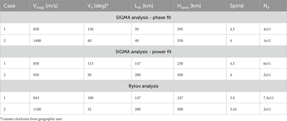
Table 2. SIGMA-derived and Rytov estimated parameters for Case 1 and Case 2 events.

For the phase fit, the PSD was derived using a 30-s segment of the phase time series from SIGMA and fitted with a 30-s observed PSD derived from SAGA observations. However, for the power fit, the PSD was computed using only 15 s of the power time series and fitted with the PSD derived from the last 15 s of the observed power time series, where significant power fluctuations were observed. This shorter window was chosen to isolate the short-lived, burst-like amplitude scintillations, which typically last only a few seconds. Using a longer interval would smear these diffractive features, reducing the ability to reproduce their spectral characteristics. This approach allows the model to find the best fit for the times where the active fluctuations of the signal power are happening, which are particularly relevant for diffractive structures.

Figure 2 shows the PSDs of observed (red) vs. simulated (blue) of phase (top row) and power (bottom row) for Case 1 and Case 2. For Case 1, the PSD of phase fluctuations (top-left) demonstrates strong agreement between the model and the observations, with a ${\chi }^{\prime }$ value of 1.24 (${\chi }^{\prime }$ close to 1 is considered as a best fit). The PSD of power fluctuations (bottom-left), for the last 15-s interval of enhanced power fluctuations, shows a good fit with observations indicating that the model captures the key features of small-scale irregularities that drive diffractive effects. Similar observations can be seen in Case 2.

Figure 2

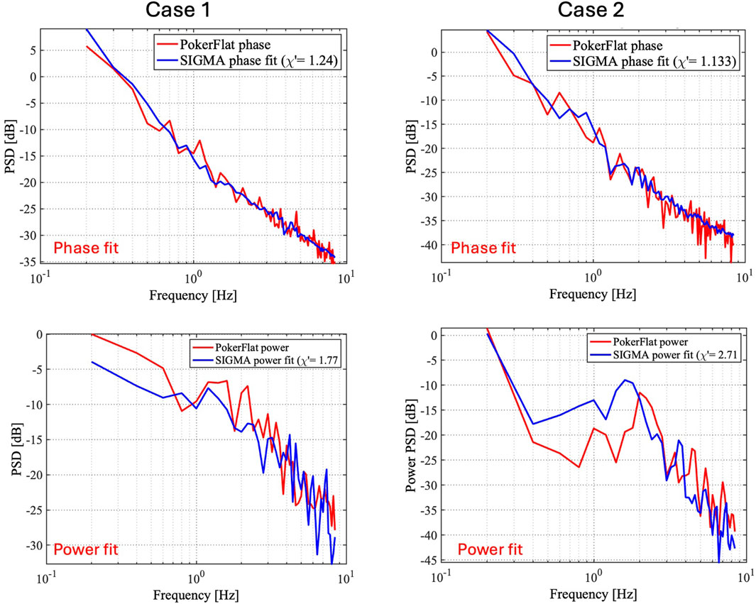
Figure 2. SIGMA best fits for Case 1 and Case 2. Top panels show phase PSD fits using 30-s segments, and bottom panels show power PSD fits using 15-s segments corresponding to the intervals of strongest amplitude scintillation. Red curves represent observed spectra and blue curves represent SIGMA simulations. Both cases demonstrate good agreement in reproducing the overall spectral shape, with power fits capturing the localized, short-lived diffractive bursts.

The estimated best-fit parameters (Table 2) can be compared with those obtained from the Rytov analysis, summarized in Table 1. It is important to note that the Rytov method yields a two-dimensional (2D) spectral index, whereas SIGMA applies a three-dimensional (3D) model. By definition, the 3D spectral index is typically one unit greater than the 2D spectral index, as discussed in Yeh and Liu (1982) and Wernik et al. (2004).

For Case 1 power fit, the drift speed was nearly identical (843 vs. $850$m/s), and both methods gave the same thickness ($147$km) and nearly the same height (247 vs. $250$km). In contrast, the SIGMA phase fit required a much thinner layer ($50$km vs. $147$km) at slightly higher altitude (295 vs. $247$km). When accounting for dimensional scaling (adding $+1$ to the 2D Rytov index), the spectral indices are in closer agreement, where Rytov gives 4.4 compared with the SIGMA value of 4.5. The electron number density from the power fit was also consistent, though slightly lower ($6\times 10^{11}$ vs. $7.3\times 10^{11}$ ${\text{m}}^{-3}$). For Case 2, the SIGMA power fit again showed closer agreement with the Rytov parameters, reproducing both the thickness ($200$km) and height ($500$km) exactly, while the drift speed (950 vs. $1100$m/s) and drift direction ($50°$ vs. $32°$) were within the expected variability. The SIGMA phase fit, by contrast, required a much thinner layer ($40$km vs. $200$km) at lower altitude (350 vs. $500$km) with a higher drift speed (1,400 vs. $1100$m/s). The spectral indices are consistent with SIGMA values (4.0 vs. 4.1).

Overall, in both cases, the SIGMA power fit reproduced the Rytov estimates more closely than the phase fit. This may be attributed to the localized and transient nature of power fluctuations, which reflects small-scale structuring occurring over short spatial and temporal scales. This comparison highlights the potential of Rytov-based estimates to provide physically meaningful initial conditions for inverse modeling. Furthermore, the need for a thicker irregularity layer and its height in the SIGMA to better estimate the spectrum of power fluctuations, as suggested by Rytov, reinforces the importance of density structuring in modeling diffractive scintillation features.

3.2 Energy cascading and structure formation

To explore the scale-dependent nature of the observed fluctuations, we segmented the 30-s time series of Figure 1 into two intervals, as shown in Figures 3a–d. These intervals isolate two distinct fluctuation regimes: one dominated by large-scale features and another where both large- and small-scale structures coexist, providing a means to investigate the presence of multiscale plasma structuring and energy cascading.

Figure 3

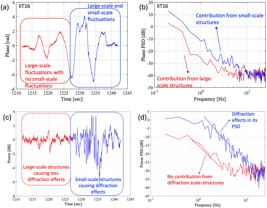
Figure 3. Phase and power fluctuations for Case 1, segmented into two 15-s intervals (red and blue, respectively). Panels (a,c) shows the time series data. Panels (b,d) shows their corresponding PSDs. The red interval is refractive-dominated, showing smooth phase variations with spectral power confined to low frequencies. The blue interval contains both refractive and diffractive components, with enhanced spectral energy at higher frequencies, indicating the onset of small-scale irregularities and stronger amplitude scintillation.

The red interval exhibits smooth phase variations with a period of $\sim 5$ seconds. These fluctuations represent refractive-scale structures typically associated with rapid gradients in Total Electron Content (TEC) or large/meso-scale field-aligned density depletions. The corresponding phase PSD confirms this behavior, with spectral power concentrated in the lower frequency regime ($\sim 0.2-1$Hz) and a rapid decline beyond $\sim 2$ Hz. The absence of significant spectral energy at higher frequencies suggests that small-scale, diffractive structures are either absent or weakly developed during this interval. This is consistent with a scenario in which the plasma structuring remains in relatively linear or early stages.

In contrast, the blue interval contains high-frequency ($\sim 2$ Hz) perturbations superimposed upon the underlying large-scale phase structure. The PSD corresponding to this segment reveals relatively enhanced spectral energy levels across both low and high frequencies, indicating the coexistence of refractive and diffractive contributions. This broader spectral regime is indicative of a more developed turbulent structuring, where energy injected at large scales is redistributed across smaller scales through nonlinear interactions, a process consistent with the concept of energy cascading in plasma turbulence, which is known to cause strong amplitude scintillation through diffractive processes.

The comparison between the two intervals thus explains the transition in the ionospheric plasma from a refractive-dominated to a refractive-plus-diffractive regime, offering observational evidence of energy transfer across scales. From an operational standpoint, these transitions from refractive-dominated to a refractive-plus-diffractive regime mark intervals when amplitude scintillation is strongest, posing a greater potential risk for GNSS signal tracking and positioning accuracy. Identifying such signatures may aid in forecasting scintillation impacts on navigation systems. This insight contributes to the broader understanding of a temporal development from large-scale (TEC) structuring toward a developed turbulent state, possibly via plasma instability mechanisms such as GDI or KHI. These mechanisms are known to facilitate the subsequent development of smaller-scale structures through secondary instabilities or nonlinear mode coupling (Basu et al., 1999; Kintner et al., 2007; Moen et al., 2013; Deshpande and Zettergren, 2019; Spicher et al., 2020).

Following the spectral analysis of phase fluctuations, we now examine the corresponding power variations to further explain the role of diffractive-scale irregularities. Figures 3c,d shows the power time series and PSDs for the first 15 s (red) and the last 15 s (blue) of the event. During the red interval, the power time series remains largely unperturbed. This behavior aligns with the absence of high-frequency perturbations in the phase signal during this period. The associated PSD of first 15-s power fluctuations (red line PSD) shows a steep decline with frequency and remains near the noise floor above $\sim 3$ Hz, indicating negligible contributions from small-scale, diffractive structures. This spectral profile suggests that the ionospheric irregularities present during this interval are predominantly large-scale, resulting in a relatively undisturbed signal power. In contrast, the blue interval (the latter 15 s) exhibits significant power fluctuations, temporally consistent with the onset of high-frequency components in phase, suggesting a strong correlation between phase and amplitude scintillation processes. The corresponding PSD (blue) shows a significant increase in spectral energy across a broad frequency range, particularly a significant energy retained in the high-frequency regime (above 1 Hz).

We further explored the respective scale sizes to determine the dominant scales that are driving large- and small-scale fluctuations. For example, the drift velocity for this case is $850$m/s, and the corresponding scales that are dominant at $2$Hz frequency are of the scale sizes of $425$m $(v/f)$. This is, of course, with an assumption that the irregularities are frozen along the magnetic field lines (frozen-in assumption). Assuming that the diffractive region starts at or above $2$Hz (and upto $10$Hz), then the small-scale irregularities that produce power fluctuations could range between $425$m and $85$m. At the large-scale regime, the scales can range between $425$m and $8.5$km (frequency of $2$Hz to $0.1$Hz), which are not diffractive and are likely to be fast-moving TEC.

Overall, we emphasize that the simultaneous occurrence of phase and power fluctuations suggests the presence of small-scale irregularities superimposed on large-scale TEC variations. The large-scale TEC structures primarily influence the phase fluctuations, while power fluctuations are driven by small-scale irregularities. The trend in power and phase time series (Figures 3a,c blue box) indicates that the strength of small-scale irregularities may be influenced by the background TEC, producing power fluctuations that exhibit both high-frequency variations and a broader, large-scale envelope. We interpret this as the irregularities represent a fast-moving plasma patch extending over a thick ionospheric region, where a local plasma instability, such as KHI and/or GDI, acts upon large-scale, precipitation-driven density structures, generating both refractive phase fluctuations from rapidly varying TEC and diffractive-scale irregularities that contribute to the observed power fluctuations.

Nishimura et al. (2023) propose that 1-min S4 (amplitude scintillation index) is not sufficient to detect scintillations. At least 1 s S4 scintillation index is needed to determine amplitude scintillations. As can be seen from the discussion above, our reported amplitude scintillations even though strong, are only occurring for less than 15-s. In order to not get washed out in the noise floor, it is recommended even for high rate (50-Hz or higher) data to look for the amplitude scintillations continually over a few seconds at a time and not over minutes-long periods of time.

3.3 Case 1 vs. Case 2 power fluctuations

In this section, we discuss our examination of power fluctuations and their spectra for Case 1 and Case 2. We strongly believe there is a relationship between phase and power fluctuations, especially highlighting the onset of high-frequency components within the phase signal that coincide with power fluctuations, as discussed in Section 2.2. It shows that the phase signal transitions from smooth to rapid fluctuations just as the power fluctuations begin, indicating a possible cascading in the plasma structuring. The power fluctuations themselves are different for the two cases when examined closely with their PSDs. There appears to be a spectral transition (or “break”) in Case 1 PSD, indicating a two-slope spectrum (Figure 4a) when compared to Case 2 with a single slope (Figure 4b).

Figure 4

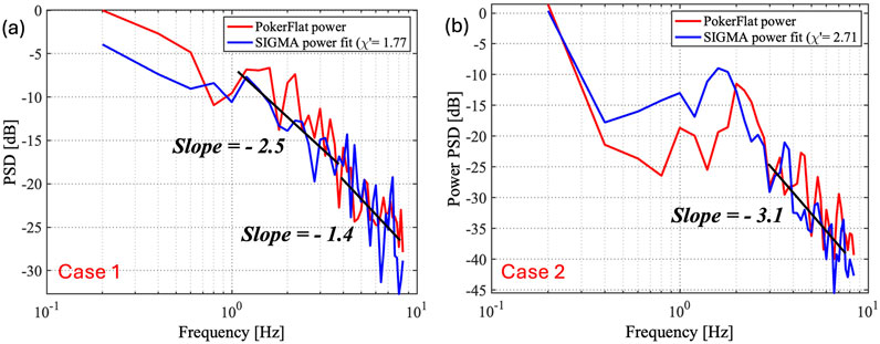
Figure 4. PSD of power fluctuations indicating the approximate spectral slopes for Case 1 and Case 2, shown in panels (a,b), respectively. Case 1 shows a two-slope spectrum with a break near $\sim 4$ Hz, separating intermediate- and small-scale irregularities. Case 2 exhibits a single-slope spectrum dominated by small-scale structures.

We calculate a linearly fitted slope at frequencies ranging from $\sim 1$Hz to $\sim 8.5$ Hz. In Case 1, a steeper slope from $\sim 1$ Hz to $\sim 4$ Hz, corresponding to intermediate-scale irregularities and a shallower slope beyond $\sim 4$ Hz, indicates the smaller scales reaching the dissipation regime. The break in spectral slope around $\sim 4$ Hz likely represents a transition between the range of irregularity scales (Carrano and Rino, 2016). In contrast, Case 2 suggests a single-slope spectrum, possibly dominated by small-scale structures or a narrower range of contributing scale sizes- likely arising from localized density gradients (e.g., structures from the tail-side region of a fully developed gradient-drift instability). The spectral slopes obtained from these two observations are consistent with those derived using the Rytov method, both representing two-dimensional (2D) spectral indices. In contrast, the SIGMA model employs a three-dimensional (3D) irregularity spectrum, where the spectral index is typically one unit greater than the corresponding 2D value. This dimensional scaling is theoretically expected and supported by previous studies (Yeh and Liu, 1982; Wernik et al., 2004; Rino, 2011).

3.4 Similar cases from SAGA data

In this section, we present a few additional examples from SAGA data where both power and phase time series exhibited strong fluctuations.

Figure 5 shows these different cases, which are similar to the two we have analyzed in detail in this paper. The events shown here are: (a) 16 November 2014 at 01:17:00 UTC (Rx IIT11), (b) 21 February 2014 at 13:21:00 UTC (Rx IIT1), (c) 19 February 2014 at 09:08:45 UTC (Rx IIT15), (d) 20 February 2014 at 07:57:25 UTC (Rx IIT11). These observations are taken from multiple SAGA receivers available during the scintillation interval (ex, IIT-1, IIT-11, etc.). Each of these events exhibits phase fluctuations, either followed by or preceded by short-duration amplitude scintillation bursts lasting approximately 3–10 s. These observations support our broader findings that the phase fluctuations are accompanied by power fluctuations, suggesting multiscale structuring or energy cascading. This behavior is particularly significant at high latitudes, where power fluctuations tend to manifest as short, high-rate bursts superimposed on longer-lasting phase trends. Despite their importance, these events are not ideal candidates for SIGMA inverse analysis due to the very short duration of fluctuations in signal power (poor spectral resolution).

Figure 5

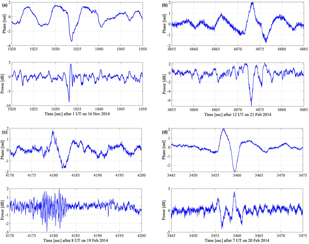
Figure 5. Panels (a–d) displays similar phase and power fluctuation events recorded by SAGA. Each of these events exhibits simultaneous phase and power fluctuations.

3.5 Limitations and modeling assumptions

This study assumes that ionospheric irregularities are represented as a uniform, slab-like layer with fixed height and thickness. A frozen-in flow assumption (Taylor’s hypothesis) is applied, where plasma irregularities are considered to drift past the receiver at a constant velocity without changing their structure during the observation window. While such assumptions are standard in scintillation modeling, they may not fully capture the spatiotemporal complexity of dynamic auroral environments.

The SIGMA forward model operates on a four-dimensional parameter space, characterizing ionospheric irregularities using electron density fluctuation strength, drift speed, drift direction, and spectral index. These four parameters are varied in the model, while five other parameters, namely, layer height, thickness, outer scale, axial ratio, and number of layers are held constant during SIGMA inversion. Sensitivity studies (Deshpande et al., 2016) have shown that the four fitted parameters have the dominant influence on GNSS signal fluctuations under typical high-latitude conditions. Additionally, a practical limitation of this study comes from the data availability, where the inversion method requires at least continuous $30$second segments of high-rate GNSS data. In amplitude scintillation cases, short-lived bursts were only captured in part of the full window. To resolve these features without smearing their spectral characteristics, we split the power spectrum into shorter intervals. Future studies incorporating time-dependent drift speeds and evolving irregularity structures may enhance the robustness of inverse modeling under disturbed conditions.

4 Conclusion and future study

This study presents a preliminary investigation of ionospheric irregularity physics using the Rytov method combined with SIGMA modeling. We identified events in the auroral region exhibiting simultaneous occurrence of phase and power fluctuations, recorded across multiple SAGA receivers. These events are particularly notable for displaying short-scale diffractive structures superimposed upon large-scale refractive phase fluctuations. Using the spectrum of observed fluctuations, we implemented the Rytov method to estimate irregularity parameters. These Rytov-derived parameters were then used as initial inputs to the SIGMA inverse modeling, which provides optimal values of the irregularity parameters by fitting simulated PSD to the observations. This combined approach demonstrated better agreement with observations, particularly when auxiliary measurements are unavailable. Moreover, by splitting the 30-s scintillation intervals, we analyzed two regimes: one dominated by large/mesoscale structures (tens of kilometers), responsible for refractive effects, and another exhibiting multiscale behavior dominated by small-scale structures, responsible for diffractive effects. The transition of large/mesoscale structures to small-scale structures reflects the cascading of turbulent energy, supporting the idea that plasma structuring processes such as gradient-drift and/or Kelvin-Helmholtz plasma instabilities drive the development of scintillation-inducing irregularities. From an operational perspective, the phase and amplitude scintillation events coincide with the conditions most prone to GNSS signal loss and navigation errors, highlighting the importance of identifying their spectral signatures for use in scintillation forecasting. Overall, this study demonstrates the effectiveness of integrating analytical Rytov-based spectral analysis with forward propagation inverse modeling for characterizing the multiscale spatial structures and their impact on GNSS signals in the high-latitude ionosphere. Looking ahead, this methodology can be extended by incorporating physics-based plasma simulations that model multiscale structuring driven by GDI and KHI. More auxiliary observations, such as ISR and all-sky imagery (ASI), enable a more comprehensive connection between the wide range of irregularity scales. Incorporating multi-year datasets to establish statistical occurrence rates of such rare events would be highly valuable. While existing studies primarily use low-rate indices, future studies incorporating high-rate observations ($50$Hz or higher) will be particularly important for capturing the short-lived, burst-like amplitude scintillations that last only a few seconds. Such integration has the potential to bring new insights into multiscale plasma dynamics and the role of energy cascading in the high-latitude ionosphere, and to contribute toward bridging the gap between physical modeling of plasma turbulence and the practical forecasting of scintillation impacts on GNSS systems.

Data availability statement

The original contributions presented in the study are publicly available. This data can be found here: https://doi.org/10.5281/zenodo.17065310.

Author contributions

PV: Writing – review and editing, Investigation, Writing – original draft, Software, Visualization, Validation, Resources, Methodology. GB: Writing – review and editing, Software, Conceptualization, Supervision, Funding acquisition, Resources, Project administration, Methodology, Visualization. KD: Writing – review and editing, Funding acquisition, Resources, Project administration, Software, Visualization, Conceptualization, Methodology, Supervision, Validation, Investigation. SD-B: Resources, Writing – review and editing, Funding acquisition, Data curation, Conceptualization, Project administration. MZ: Writing – review and editing, Supervision.

Funding

The author(s) declare that financial support was received for the research and/or publication of this article. We gratefully acknowledge support from the NSF under grants AGS-1651465, AGS-1651410, AGS-1651466, and AGS-1651448, as well as from NASA under grant 80NSSC21K1354.

Acknowledgments

We thank Embry-Riddle Aeronautical University for providing access to the VEGA high-performance computing facility, which was helpful in carrying out the simulations for this study.

Conflict of interest

The authors declare that the research was conducted in the absence of any commercial or financial relationships that could be construed as a potential conflict of interest.

Generative AI statement

The author(s) declare that no Generative AI was used in the creation of this manuscript.

Any alternative text (alt text) provided alongside figures in this article has been generated by Frontiers with the support of artificial intelligence and reasonable efforts have been made to ensure accuracy, including review by the authors wherever possible. If you identify any issues, please contact us.

Publisher’s note

All claims expressed in this article are solely those of the authors and do not necessarily represent those of their affiliated organizations, or those of the publisher, the editors and the reviewers. Any product that may be evaluated in this article, or claim that may be made by its manufacturer, is not guaranteed or endorsed by the publisher.

References

Aaron, J. (1982). Global morphology of ionospheric scintillations. Proc. IEEE 70, 360–378. doi:10.1109/proc.1982.12314

CrossRef Full Text | Google Scholar

Basu, S., Basu, S., McClure, J., Hanson, W., and Whitney, H. (1983). High resolution topside in situ data of electron densities and vhf/ghz scintillations in the equatorial region. J. Geophys. Res. Space Phys. 88, 403–415. doi:10.1029/ja088ia01p00403

CrossRef Full Text | Google Scholar

Basu, S., Groves, K., Quinn, J., and Doherty, P. (1999). A comparison of tec fluctuations and scintillations at Ascension island. J. Atmos. Solar-Terrestrial Phys. 61, 1219–1226. doi:10.1016/s1364-6826(99)00052-8

CrossRef Full Text | Google Scholar

Bhattacharyya, A., Beach, T., Basu, S., and Kintner, P. (2000). Nighttime equatorial ionosphere: gps scintillations and differential carrier phase fluctuations. Radio Sci. 35, 209–224. doi:10.1029/1999rs002213

CrossRef Full Text | Google Scholar

Carlson, H. C., Pedersen, T., Basu, S., Keskinen, M., and Moen, J. (2007). Case for a new process, not mechanism, for cusp irregularity production. J. Geophys. Res. Space Phys. 112. doi:10.1029/2007ja012384

CrossRef Full Text | Google Scholar

Carrano, C. S., and Rino, C. L. (2016). A theory of scintillation for two-component power law irregularity spectra: overview and numerical results. Radio Sci. 51, 789–813. doi:10.1002/2015rs005903

CrossRef Full Text | Google Scholar

Costa, E., Fougere, P. F., and Basu, S. (1988). Cross-correlation analysis and interpretation of spaced-receiver measurements. Radio Sci. 23, 141–162. doi:10.1029/rs023i002p00141

CrossRef Full Text | Google Scholar

Datta-Barua, S., Su, Y., Deshpande, K., Miladinovich, D., Bust, G., Hampton, D., et al. (2015). First light from a kilometer-baseline scintillation auroral gps array. Geophys. Res. Lett. 42, 3639–3646. doi:10.1002/2015gl063556

PubMed Abstract | CrossRef Full Text | Google Scholar

Datta-Barua, S., Su, Y., Rubio, A. L., and Bust, G. S. (2020). Ionospheric irregularity layer height and thickness estimation with a gnss receiver array. IEEE Trans. Geoscience Remote Sens. 59, 6198–6207. doi:10.1109/tgrs.2020.3024173

CrossRef Full Text | Google Scholar

Datta-Barua, S., Prat, P. L., and Hampton, D. L. (2021). Multiyear detection, classification and hypothesis of ionospheric layer causing gnss scintillation. Radio Sci. 56, 1–11. doi:10.1029/2021RS007328

CrossRef Full Text | Google Scholar

De Franceschi, G., Spogli, L., Alfonsi, L., Romano, V., Cesaroni, C., and Hunstad, I. (2019). The ionospheric irregularities climatology over Svalbard from solar cycle 23. Sci. Rep. 9, 9232. doi:10.1038/s41598-019-44829-5

PubMed Abstract | CrossRef Full Text | Google Scholar

Deshpande, K. B., and Zettergren, M. D. (2019). Satellite-beacon ionospheric-scintillation global model of the upper atmosphere (sigma) iii: scintillation simulation using a physics-based plasma model. Geophys. Res. Lett. 46, 4564–4572. doi:10.1029/2019gl082576

CrossRef Full Text | Google Scholar

Deshpande, K., Bust, G., Clauer, C., Kim, H., Macon, J., Humphreys, T., et al. (2012). Initial gps scintillation results from cases receiver at south pole, Antarctica. Radio Sci. 47, 2012RS005061–10. doi:10.1029/2012rs005061

CrossRef Full Text | Google Scholar

Deshpande, K., Bust, G., Clauer, C., Rino, C., and Carrano, C. (2014). Satellite-beacon ionospheric-scintillation global model of the upper atmosphere (sigma) i: high-latitude sensitivity study of the model parameters. J. Geophys. Res. Space Phys. 119, 4026–4043. doi:10.1002/2013ja019699

CrossRef Full Text | Google Scholar

Deshpande, K., Bust, G., Clauer, C., Scales, W., Frissell, N., Ruohoniemi, J., et al. (2016). Satellite-beacon ionospheric-scintillation global model of the upper atmosphere (sigma) ii: inverse modeling with high-latitude observations to deduce irregularity physics. J. Geophys. Res. Space Phys. 121, 9188–9203. doi:10.1002/2016ja022943

CrossRef Full Text | Google Scholar

Enengl, F., Spogli, L., Kotova, D., Jin, Y., Oksavik, K., Partamies, N., et al. (2024). Investigation of ionospheric small-scale plasma structures associated with particle precipitation. Space Weather. 22, e2023SW003605. doi:10.1029/2023sw003605

CrossRef Full Text | Google Scholar

Ghobadi, H., Spogli, L., Alfonsi, L., Cesaroni, C., Cicone, A., Linty, N., et al. (2020). Disentangling ionospheric refraction and diffraction effects in gnss raw phase through fast iterative filtering technique. GPS Solutions 24, 85. doi:10.1007/s10291-020-01001-1

CrossRef Full Text | Google Scholar

Ishimaru, A. (1978). Wave propagation and scattering in random media, 2. New York: Academic Press.

Google Scholar

Jiao, Y., Morton, Y. T., Taylor, S., and Pelgrum, W. (2013). Characterization of high-latitude ionospheric scintillation of gps signals. Radio Sci. 48, 698–708. doi:10.1002/2013rs005259

CrossRef Full Text | Google Scholar

Kintner, P. M., and Seyler, C. E. (1985). The status of observations and theory of high latitude ionospheric and magnetospheric plasma turbulence. Space Sci. Rev. 41, 91–129. doi:10.1007/bf00241347

CrossRef Full Text | Google Scholar

Kintner, P. M., Ledvina, B. M., and De Paula, E. (2007). Gps and ionospheric scintillations. Space Weather. 5. doi:10.1029/2006sw000260

CrossRef Full Text | Google Scholar

McCaffrey, A. M., and Jayachandran, P. (2017). Spectral characteristics of auroral region scintillation using 100 hz sampling. GPS Solutions 21, 1883–1894. doi:10.1007/s10291-017-0664-z

CrossRef Full Text | Google Scholar

Moen, J., Oksavik, K., Alfonsi, L., Daabakk, Y., Romano, V., and Spogli, L. (2013). Space weather challenges of the polar cap ionosphere. J. Space Weather Space Clim. 3, A02. doi:10.1051/swsc/2013025

CrossRef Full Text | Google Scholar

Nishimura, Y., Kelly, T., Jayachandran, P., Mrak, S., Semeter, J. L., Donovan, E., et al. (2023). Nightside high-latitude phase and amplitude scintillation during a substorm using 1-second scintillation indices. J. Geophys. Res. Space Phys. 128, e2023JA031402. doi:10.1029/2023ja031402

CrossRef Full Text | Google Scholar

Press, W. H. (2007). “Numerical recipes,” in The art of scientific computing. 3rd edition (Cambridge: Cambridge University Press).

Google Scholar

Rino, C. (1979). A power law phase screen model for ionospheric scintillation: 1. weak scatter. Radio Sci. 14, 1135–1145. doi:10.1029/rs014i006p01135

CrossRef Full Text | Google Scholar

Rino, C. (2011). The theory of scintillation with applications in remote sensing. John Wiley and Sons.

Google Scholar

Rufenach, C. L. (1975). Ionospheric scintillation by a random phase screen: spectral approach. Radio Sci. 10, 155–165. doi:10.1029/rs010i002p00155

CrossRef Full Text | Google Scholar

Spicher, A., Miloch, W., and Moen, J. (2014). Direct evidence of double-slope power spectra in the high-latitude ionospheric plasma. Geophys. Res. Lett. 41, 1406–1412. doi:10.1002/2014gl059214

CrossRef Full Text | Google Scholar

Spicher, A., Deshpande, K., Jin, Y., Oksavik, K., Zettergren, M. D., Clausen, L. B., et al. (2020). On the production of ionospheric irregularities via kelvin-helmholtz instability associated with cusp flow channels. J. Geophys. Res. Space Phys. 125, e2019JA027734. doi:10.1029/2019ja027734

CrossRef Full Text | Google Scholar

Sreenivash, V., Su, Y., and Datta-Barua, S. (2020). Automated ionospheric scattering layer hypothesis generation for detected and classified auroral global positioning system scintillation events. Radio Sci. 55, 1–15. doi:10.1029/2018RS006779

CrossRef Full Text | Google Scholar

Tatarski, V. I. (2016). Wave propagation in a turbulent medium. Courier Dover Publications.

Google Scholar

Tatarskii, V. I. (1971). The effects of the turbulent atmosphere on wave propagation. Jerusalem: Israel Program for Scientific Translations.

Google Scholar

Taylor, G. I. (1938). The spectrum of turbulence. Proc. R. Soc. Lond. Ser. A-Mathematical Phys. Sci. 164, 476–490. doi:10.1098/rspa.1938.0032

CrossRef Full Text | Google Scholar

Taylor, L. S. (1975). Effects of layered turbulence on oblique waves. Radio Sci. 10, 121–128. doi:10.1029/rs010i001p00121

CrossRef Full Text | Google Scholar

Tsunoda, R. T. (1988). High-latitude f region irregularities: a review and synthesis. Rev. Geophys. 26, 719–760. doi:10.1029/rg026i004p00719

CrossRef Full Text | Google Scholar

Vaggu, P. R., Deshpande, K. B., Datta-Barua, S., Bust, G. S., Hampton, D. L., Rubio, A. L., et al. (2023). Morphological and spectral features of ionospheric structures at e-and f-region altitudes over poker flat analyzed using modeling and observations. Sensors 23, 2477. doi:10.3390/s23052477

PubMed Abstract | CrossRef Full Text | Google Scholar

Vaggu, P. R., Zettergren, M., Deshpande, K., Nishimura, Y., Semeter, J., Hirsch, M., et al. (2024). Model-based investigation of electron precipitation-driven density structures and their effects on auroral scintillation. J. Geophys. Res. Space Phys. 129, e2024JA032443. doi:10.1029/2024ja032443

CrossRef Full Text | Google Scholar

van der Meeren, C., Oksavik, K., Lorentzen, D., Moen, J. I., and Romano, V. (2014). Gps scintillation and irregularities at the front of an ionization tongue in the nightside polar ionosphere. J. Geophys. Res. Space Phys. 119, 8624–8636. doi:10.1002/2014ja020114

CrossRef Full Text | Google Scholar

Van Dierendonck, A., Klobuchar, J., and Hua, Q. (1993). Ionospheric scintillation monitoring using commercial single frequency c/a code receivers. Proc. ION GPS 93, 1333–1342.

Google Scholar

Wernik, A., Secan, J., and Fremouw, E. (2003). Ionospheric irregularities and scintillation. Adv. Space Res. 31, 971–981. doi:10.1016/s0273-1177(02)00795-0

CrossRef Full Text | Google Scholar

Wernik, A. W., Alfonsi, L., and Materassi, M. (2004). Ionospheric irregularities, scintillation and its effect on systems. Acta Geophys. Pol. 52, 237–249.

Google Scholar

Yeh, K. C., and Liu, C.-H. (1982). Radio wave scintillations in the ionosphere. Proc. IEEE 70, 324–360. doi:10.1109/proc.1982.12313

CrossRef Full Text | Google Scholar

Nomenclature

Abbreviations/acronyms

GPS Global Positioning System

GNSS Global Navigation Satellite System

PSD Power Spectral Density

PFISR Poker Flat Incoherent Scatter Radar

SAGA Scintillation Auroral GPS Array

SIGMA Satellite-beacon Ionospheric-scintillation Global Model of the upper Atmosphere

TEC Total Electron Content

GDI Gradient-Drift Instability

KHI Kelvin–Helmholtz Instability

Symbols and parameters

$|{\mathit{v}}_{\mathit{d}}|/{\mathit{V}}_{\mathit{mag}}$ Drift speed

$\mathit{\angle }{\mathit{v}}_{\mathit{d}}/{\mathit{V}}_{\mathit{\theta }}$ Drift direction (measured counterclockwise from geographic east)

$\mathit{L}/{\mathit{L}}_{\mathit{t}\mathit{h}}$ Irregularity layer thickness

$\mathit{z}/{\mathit{H}}_{\mathit{iono}}$ Height of the irregularity layer (ionospheric altitude)

$\mathit{S}\mathit{p}\mathit{I}\mathit{n}\mathit{d}$ Spectral index of electron density irregularities

${\mathit{N}}_{\mathit{e}}$ RMS electron number density fluctuations

$\mathit{\lambda }$ Wavelength

$\mathit{k}$ Free-space wavenumber $(2\pi /\lambda )$

${\mathit{k}}_{\Vert }$ Wave vector component along propagation direction

${\mathit{k}}_{\perp }$ Perpendicular wave vector

$\mathit{\varphi }$ Azimuth angle of wave propagation

$\mathit{\theta }$ Zenith angle of propagation