Adaptive extended Kalman filter and laser link acquisition in the detection of gravitational waves in space

Introduction: Establishing stable laser links in triangular spacecraft constellations for gravitational wave detection is challenging due to large initial pointing uncertainties and the limitations of conventional acquisition schemes.

Methods: We propose an alternative acquisition scheme that replaces the wide-field CCD camera with an adaptive extended Kalman filter (AEKF) integrated into the point-ahead angle mechanism (PAAM). The scheme employs a quadrant photodetector (QPD) based on differential power sensing (DPS), which provides a higher dynamic range than differential wavefront sensing (DWS).

Results: By integrating coarse and fine acquisition into a single control loop, the payload structure of the acquisition, tracking, and pointing (ATP) system is simplified. Numerical simulations using a colored measurement noise model, representative of on-orbit conditions, show that the AEKF effectively predicts the point-ahead angle (PAA) and significantly reduces the initial uncertainty region, even under worst-case spacecraft navigation errors.

Discussion: The proposed scheme avoids CCD-induced heating issues, enhances robustness against navigation errors, and offers a simplified yet efficient approach for deep-space laser link acquisition in gravitational wave detection missions.

1 Introduction

In the detection of gravitational waves in space, a triangular constellation of SCs with laser links among them serves as a laser interferometer to detect the picometer-scale miniature change in armlength between two SCs generated by variation in the spacetime curvature of a gravitational wave sources (Luo et al., 2020; Danzmann and Team, 1996; Luo et al., 2016). In the initial phase of the mission, laser link acquisition is required for SCs of millions of kilometers away from each other before the scientific phase of the mission employing laser interferometry can take place.

In the conventional strategy (Cirillo and Gath, 2009; Hu et al., 2024; Gao et al., 2021b), a key payload is the CCD camera with a wide field angle, which serves to narrow the angle of the uncertainty cone from $mrad$ to $\mu rad$, and then the scan by the laser beam takes over. The problem with the CCD camera is the heat generated. Due to a lack of heat ventilation in space, a specific metallic tube structure is required to channel the heat out of SC, and this complicates the payload structure. Further, the experience of the heating problem of the thrusters in LPF suggests that the thermal gradient generated will take some time to die out (Gao et al., 2021a; Ales et al., 2014; Luo et al., 2017) and the scientific phase of the mission will have to wait until the thermal stability of the SC is restored. A further disadvantage is that once the laser link acquisition is established, the CCD camera will become redundant and no longer play any role in the scientific phase of the mission.

Current research on space-based gravitational wave detection has focused mainly on simulation and preliminary verification of link acquisition schemes. Cirillo designed Kalman-filter-based controllers for the LISA acquisition phase and demonstrated their effectiveness through simulations (Cirillo and Gath, 2009). For the Taiji program, Gao developed a ground-based acquisition and pointing testbed to verify methodological feasibility (Gao et al., 2021a, Luo et al., 2017). In addition, Hu designed a device to emulate inter-satellite laser beam propagation and experimentally validated a bidirectional link acquisition scheme using an acquisition camera and the QPD based on the DWS technology (Hu et al., 2024). At present, no research has explored using orbit determination information to assist in the establishment of inter-satellite optical laser links in space-based gravitational wave detection. The aim of the present work is to look into the feasibility of replacing the CCD camera by the PAAM with an AEKF based on precision orbit determination in deep space incorporated into it. In the scientific phase, the PAAM serves to steer a laser beam to compensate for the angle generated by the relative motion between two SCs during the time it takes (around 10 s) for a laser beam to travel from a SC to a distant one. It also plays a role in compensating for the breathing angle at the annual level due to solar gravity (Yang et al., 2024; Hechenblaikner et al., 2023). In this work, we will try to understand the possible role PAAM can play even at the stage of laser link acquisition, with the aid of an AEKF. This will avoid the heating problem generated by a CCD camera and simplify the payload structure of SC.

The structure of this paper is organized as follows. Some background materials concerning ATP and scanning strategy are introduced in Sections 2, 3, respectively. We begin to enter the core of our work in Section 4, presenting the AEKF model with colored noise, the ATP control loop, and the noise model. Section 5 presents the simulation results and conducts an in-depth analysis of the scanning time results obtained from AEKF. In the final section, some remarks that look to the future of this work are made to conclude our work.

2 Payload structure of the laser link acquisition for inter-satellite laser interferometry

Figure 1 illustrates the new schematic of inter-satellite laser-ranging interferometry in our plan. In this section, we will describe the payload structure for the laser link acquisition. Apart from the PAAM and DPS angle measurement based on QPD that replaces a CCD camera, the two schemes share several payloads in common. In what follows, we shall first describe the common payloads before we go into the detailed structure of the PAAM, and the AEKF system model will also be introduced in this section.

Figure 1

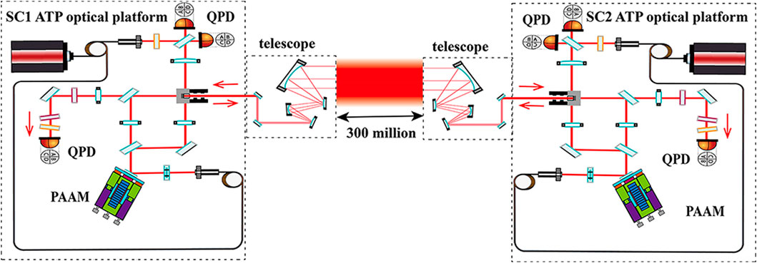
Figure 1. New schematic drawing of the laser ranging interferometry.

2.1 ATP optical bench design and process overview

Once a SC reaches its targeted position, precision orbit determination by the Deep Space Network (DSN) gives an initial position with a certain error margin. Due to launch-induced vibrations, the lasers on the two SCs initially exhibit a frequency difference in the GHz range. To mitigate this, each SC’s laser undergoes pre-stabilization, achieving a frequency stability of $30\text{\hspace{0.17em}Hz}/\sqrt{\text{Hz}}$.

After coupling into the fiber collimator, the laser is split in a 1:99 ratio. The telescope reflects $99\%$ of the laser power. The telescope, an off-axis retroreflector composed of four mirrors (Yu et al., 2024), directs the reflected beam back along the incident axis, enabling it to propagate approximately 3 million kilometers to the distant SC. The remaining $1\%$ of the laser power is directed to the fine-tracking QPD. The optical imaging system in front of the fine-tracking QPD is generally composed of either a lens system of three mirrors. Its primary function is to mitigate the impact of TTL noise, ensuring that the signal detected by the QPD reflects only the relative angular variations between the two beams. This setup effectively eliminates the influence of translational displacement between the beams.

For the receiving SC, the incoming laser beam from the transmitting SC passes through the telescope and is clipped by an aperture stop at the receiving aperture. After passing through a beam splitter (BS), it is divided into two parts. One portion is focused onto the acquisition QPD by an optical lens, while the other portion passes through a dual-lens imaging system and then interferes with the local SC’s laser on the fine-tracking QPD. The received optical power is extremely low (100 pW), making the signal-to-noise ratio a major challenge. To address this challenge, a dedicated acquisition QPD hardware design is proposed, which enhances front-end amplification and reduces quadrant noise, thereby improving readout sensitivity and overall SNR. An optical phase-locked loop (OPLL) locks the phase between the transmitting and receiving SC lasers.

2.2 The star tracker (STR)

The STR is a key component in SC’s attitude determination system. It provides high-precision attitude information by detecting and identifying stars in its field of view (FOV). Based on the in-orbit experience of the BeiDou system, the readout noise of the STR currently is at the order of $1\times 10^{-5}$ rad. In a decade or so, it is anticipated that the readout noise of a STR will be improved to $1\times 10^{-6}$ rad. By then, the PAAM together, possibly with an AEKF alone, can fully cover the uncertain region during the scanning phase, eliminating the reliance on micro-newton thrusters for attitude adjustments (Cui et al., 2024). This work will focus on STR with $1\times 10^{-5}$ rad readout noise.

2.3 The role of the telescope on the acquisition phase

The optical aperture is the primary metric for evaluating a telescope’s light-gathering capability. A larger telescope aperture allows for a greater light flux, which in turn results in higher received energy. However, since the interferometric arm length is on the order of 3 million kilometers, increasing the optical aperture alone has a minimal effect on improving the received energy but would significantly increase manufacturing challenges. Drawing on the optical aperture configurations of similar telescopes in the BeiDou system, the ATP system employs an off-axis four-mirror structure telescope with an aperture of 200 mm (Yu et al., 2024). During the capture phase, the telescope primarily influences the capture FOV and the scanning range of the PAAM.

The telescope considered will have an FOV of 400 $\mu \mathrm{r}\mathrm{a}\mathrm{d}$ (Miao et al., 2023), while the QPD, which uses DPS for angle measurement, can achieve an FOV of up to 1 $\mathrm{m}\mathrm{r}\mathrm{a}\mathrm{d}$. Therefore, during the capture phase, the size of the capture FOV is mainly determined by the telescope’s FOV. Additionally, the telescope has a magnification of 40 times. When the PAAM is used to scan the uncertainty region, the scanning range is reduced by a factor of 30 due to the telescope’s effect. Specifically, the pitch angle is reduced from $\pm 270\mu \mathrm{r}\mathrm{a}\mathrm{d}$ to $\pm 6.75\mu \mathrm{r}\mathrm{a}\mathrm{d}$, and the deflection angle is reduced from $\pm 268\mu \mathrm{r}\mathrm{a}\mathrm{d}$ to $\pm 6.75\mu \mathrm{r}\mathrm{a}\mathrm{d}$.The waist size of the emitted laser beam is comparable to the diameter of the telescope. Assuming that the beam waist radius $r$ is approximately 20 cm, the approximate half-angle divergence of the laser can be derived using Equation 1 for beam divergence in a Gaussian beam context:

${\theta }_{\text{div}}=\frac{\lambda }{r\pi }\approx 1.69\mu \mathrm{r}\mathrm{a}\mathrm{d}.(1)$

Due to the influence of SC pointing jitter and telescope pointing angle jitter, the half-angle of the actual effective beam receiving area can be approximated as the difference between the divergence angle and the angular jitter (Vinet et al., 2019). The pointing error caused by attitude jitter and angular jitter is approximately less than $0.15\mu \mathrm{r}\mathrm{a}\mathrm{d}$, and the half-angle of the effectively received beam can be expressed by Equation 2:

${\theta }_{\text{effective}}=1.54\mu \mathrm{r}\mathrm{a}\mathrm{d}.(2)$

2.4 PAAM–key distinction between the conventional strategy and the proposed one

Compared to the traditional optical platform design for the acquisition phase, there are three main differences. First, a PAAM has been added to the outgoing optical path to enhance scanning efficiency during the scanning phase in coordination with micro-newton thrusters. The specific details of the scanning process will be thoroughly discussed in what follows. Further, a PAAM monitoring interferometer has been incorporated into the original optical path, utilizing an optical closed-loop system to improve the pointing accuracy of the PAAM. The PAAM monitoring interferometer also enables the PAAM to suppress a portion of the pointing jitter noise introduced by the local optical platform through AEKF. This integration allows the pointing adjustments of both phases to be accomplished within a single phase. Finally, by inserting an AEKF into the PAAM, we can replace the CCD camera with a QPD based on DPS angle measurement technology. This substitution resolves the thermal balance issue of the optical platform and enables immediate tracking and pointing operations after the link establishment.

The PAAM should ideally be placed at the entrance pupil of the telescope, as it alters the outgoing angle of the telescope’s emitted light. Placing the PAAM at this location limits the size of the emitted beam, ensuring that the beam’s spot size within the telescope is well controlled and preventing it from striking structural components and generating stray light. Additionally, an aperture is employed to further constrain the beam’s spot size. By rotating the PAAM, the direction of the transmitted (TX) beam is adjusted.

As shown in Figure 2, PAAM as a two-dimensional motion component mounted on the optical platform that provides the PAA, is one of the key components for establishing the inter-satellite scientific interferometric link (Liu et al., 2022). It needs to address two core technical challenges: (1) Due to the extremely long arm length of the inter-satellite interferometric link, the PAA pre-pointing must achieve high-precision pointing (Wu et al., 2023). (2) The PAAM pointing assembly must maintain ultra-stable optical path stability and avoid introducing any additional optical path noise during its rotation. This is because the PAAM is directly involved in the scientific interferometer, and its optical path performance directly impacts the constellation’s detection accuracy (Liu et al., 2022). The PAAM has a deflection range of $\pm 270\mu rad$ in yaw and $\pm 268\mu rad$ in pitch, with a pointing accuracy of $0.35\mu rad$ in both axes (Zhu et al., 2024). The PAAM relies on built-in capacitance sensors to convert displacement into deflection angles for closed-loop control. Its deflection range is limited by the sensor’s measurement range, as increasing range reduces resolution and feedback accuracy. At present, domestic technology cannot provide capacitance sensors with both large range and high precision needed for an enhanced PAAM. Considering the telescope’s $40\times$ magnification factor, these ranges are reduced to $\pm 6.75\mu rad$ (yaw) and $\pm 6.75\mu rad$ (pitch), while the effective pointing accuracy is improved to $<0.012\mu rad$ for both axes. To guarantee operational reliability and prevent the degradation of piezoelectric actuators, during experiments, we limit the post - telescope operational range to $\pm 6\mu rad$ for both axes. This measure addresses two crucial constraints. First, long - term operation at maximum deflection impairs pointing accuracy. Second, extreme positions may damage the piezoelectric components. The piezoelectric actuators of the PAAM offer a rapid response ($>10kHz$ bandwidth in vacuum conditions). Nevertheless, to reduce thermal effects from sustained high-frequency operation during the ATP phase, we set the scanning speed after the telescope to $1mrad/s$.

Figure 2

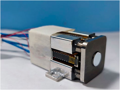
Figure 2. Physical diagram of the PAAM.

2.5 PAA calculated from orbit position and velocity information

At the initial stage of link establishment, the desired attitude of the SC is determined using dual-vector attitude determination based on the PAA and orbital determination errors. Calculating the desired attitude requires converting the SC’s position and velocity in the J2000.0 frame, along with orbit determination errors, into the PAA (Han et al., 2022).

The PAA is defined as the angle between the direction of the transmitted beam from the local SC to the remote SC and the direction of the received beam from the remote SC to the local SC, as illustrated in Figure 3. This angle varies annually with the orbit of the triangular constellation. Throughout this work, the J2000.0 coordinate system is adopted to describe the position and velocity of the SCs.

Figure 3

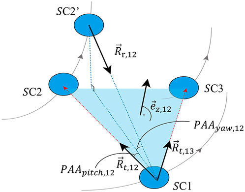
Figure 3. Definition of the point ahead angle.

The positions and velocities of the $i$-th SC (where $i=\mathrm{1,2,3}$) at a given epoch can be expressed as ${[X_i,Y_i,Z_i]}^T$ and ${[V_{Xi},V_{Yi},V_{Zi}]}^T$, respectively. The position and velocity errors caused by orbital determination errors are defined as ${[\delta X_i,\delta Y_i,\delta Z_i]}^T$ and ${[\delta V_{Xi},\delta V_{Yi},\delta V_{Zi}]}^T$. Thus, the SC position and velocity incorporating orbital determination errors can be obtained in the J2000.0 coordinate system, as shown in Equation 3.

$\left\{\begin{array}{cc}\hfill & X={\left[X_i+\delta X_i,Y_i+\delta Y_i,Z_i+\delta Z_i\right]}^T,\hfill \\ \hfill & V={\left[V_{Xi}+\delta V_{Xi},V_{Yi}+\delta V_{Yi},V_{Zi}+\delta V_{Zi}\right]}^T.\hfill \end{array}\right.(3)$

the relative position and velocity of two SCs are then given by vector addition or subtraction with respect to the J2000.0 reference frame (Yang et al., 2024). We shall divide the PAA into two parts in the calculations: yaw and pitch, as shown in Figure 3.

${\vec{R}}_{12}$ denotes the laser link vector directed from SC1 to SC2, and ${\vec{V}}_{12}$ represents the relative velocity vector between SC1 and SC2. The beam vectors ${\vec{R}}_{t,12}$ and ${\vec{R}}_{r,12}$ also describe the link from SC1 to SC2. Here, $\mathrm{\Delta }t$ denotes the laser transmission time between the two spacecraft, with variations due to relative distance changes considered negligible. Similarly, ${\vec{R}}_{t,13}$ represents the beam vector from SC1 to SC3.

To calculate the PAA of the SC, it is necessary to transform the origin of the coordinate system from the J2000.0 coordinate system to the center of mass of the SC. As shown in Figure 3, we define three unit direction vectors of the SC coordinate system as ${\vec{e}}_{x,12}$, ${\vec{e}}_{z,12}$, and ${\vec{e}}_{y,12}$ (Yang et al., 2024). The expression of ${\vec{e}}_{z,12}$ is provided by Equations 4, 5

${\vec{e}}_{z,12}=\frac{1}{{\left|{\vec{R}}_{t,12}\right|}^2\left|{\vec{R}}_{t,13}\right|}\left[\begin{array}{c}\hfill {e_z}_x\hfill \\ \hfill e_{zy}\hfill \\ \hfill e_{zz}\hfill \end{array}\right],(4)$

with

$\left[\begin{array}{c}\hfill {e_z}_x\hfill \\ \hfill e_{zy}\hfill \\ \hfill e_{zz}\hfill \end{array}\right]=\left[\begin{array}{c}\hfill \left(y_{12}+V{y}_{12}\mathrm{\Delta }t\right)\left(z_{13}+V{z}_{13}\mathrm{\Delta }t\right)-\left(z_{12}+V{z}_{12}\mathrm{\Delta }t\right)\left(y_{13}+V{y}_{13}\mathrm{\Delta }t\right)\hfill \\ \hfill \left(z_{12}+V{z}_{12}\mathrm{\Delta }t\right)\left(x_{13}+V{x}_{13}\mathrm{\Delta }t\right)-\left(x_{12}+V{x}_{12}\mathrm{\Delta }t\right)\left(z_{13}+V{z}_{13}\mathrm{\Delta }t\right)\hfill \\ \hfill \left(x_{12}+V{x}_{12}\mathrm{\Delta }t\right)\left(y_{13}+V{y}_{13}\mathrm{\Delta }t\right)-\left(y_{12}+V{y}_{12}\mathrm{\Delta }t\right)\left(x_{13}+V{x}_{13}\mathrm{\Delta }t\right)\hfill \end{array}\right].(5)$

The initial pointing pitch angle is provided by Equations 6, 7

$\begin{array}{ccc}\hfill {\text{PAA}}_{\text{\hspace{0.17em}pitch,}12}=\frac{{\vec{R}}_{r,12}}{\left|{\vec{R}}_{r,12}\right|}\times {\vec{e}}_{z,12}\cdot \frac{{\vec{R}}_{t,12}}{\left|{\vec{R}}_{t,12}\right|}& \hfill & \hfill \\ \hfill =\frac{{\vec{R}}_{r,12}\times \left({\vec{R}}_{t,12}\times {\vec{R}}_{t,13}\right)\cdot {\vec{R}}_{t,12}}{{\left|{\vec{R}}_{r,12}\right|}^2\left|{\vec{R}}_{t,13}\right|\left|{\vec{R}}_{t,12}\right|}.& \hfill & \hfill \end{array}(6)$

with

$\begin{array}{ll}\hfill & \hfill {\vec{R}}_{r,12}\times \left({\vec{R}}_{t,12}\times {\vec{R}}_{t,13}\right)\cdot {\vec{R}}_{t,12}=\left(\left(y_{12}-V_{y_{12}}\mathrm{\Delta }t\right)e_{zz}-\left(z_{12}-V_{z_{12}}\mathrm{\Delta }t\right)e_{zy}\right)\\ \hfill & \times \left(x_{12}+V{x}_{12}\mathrm{\Delta }t\right)+\left(\left(z_{12}-V_{z_{12}}\mathrm{\Delta }t\right){e_z}_x-\left(x_{12}-V{x}_{12}\mathrm{\Delta }t\right)e_{zz}\right)\left(y_{12}+V_{y_{12}}\mathrm{\Delta }t\right)\hfill \\ \hfill & +\left(\left(x_{12}-V{x}_{12}\mathrm{\Delta }t\right){e_z}_y-\left(y_{12}-V_{y_{12}}\mathrm{\Delta }t\right)e_{zx}\right)\left(z_{12}+V_{z_{12}}\mathrm{\Delta }t\right).\hfill \end{array}(7)$

The expression of the initial pointing yaw angle is provided by Equation 8

$\begin{array}{ll}\hfill & \hfill {\text{PAA}}_{\text{\hspace{0.17em}yaw,}12}=\frac{{\vec{e}}_{z,12}\cdot {\vec{R}}_{r,12}}{|{\vec{R}}_{r,12}|}\\ \hfill & =\frac{1}{\left|{\vec{R}}_{t,12}\right|\left|{\vec{R}}_{t,13}\right|\left|{\vec{R}}_{r,12}\right|}\hfill \\ \hfill & \cdot \left({e_z}_x\left(x_{12}-V_{x_{12}}\mathrm{\Delta }t\right)+{e_z}_y\left(y_{12}-V_{y_{12}}\mathrm{\Delta }t\right)+{e_z}_z\left(z_{12}-V_{z_{12}}\mathrm{\Delta }t\right)\right).\hfill \end{array}(8)$

2.6 The uncertainty cone and precison orbit determination in deep space

As illustrated in Figure 4, the size of the uncertainty region during the ATP phase is determined by the SC position (navigation) error introduced by the DSN. As the distance between the Earth and the triangle constellation is very similar to that between Mars and the Earth, the experience for the precision orbit determination of the Martian mission Tianwen I will serve as a useful reference guide (Yang et al., 2022). When the DSN performs 24-h full-arc tracking, the orbit determination accuracy of the SC can reach 50 m (Li and Zheng, 2021). When the DSN tracks for 4 h per day, the orbit determination accuracy of the SC is approximately 400 m–500 m. As the DSN performs 2 h tracking per day, the orbit determination accuracy of the SC is $2\text{\hspace{0.17em}km}$ and $0.2\text{\hspace{0.17em}cm/s}$. In an optimal scenario when the DSN performs 24-h trajectory tracking of the SC, the link establishment can be accomplished directly using the PAAM, without the need for an AEKF. In this work, we will consider the case when the initial orbit error is $2\text{\hspace{0.17em}km}$ and $0.2\text{\hspace{0.17em}cm/s}$ as input into the AEKF orbital integrator. Our scheme remains effective even under less optimal conditions, where the SC’s orbit determination accuracy is $20\text{\hspace{0.17em}km}$ and $0.2\text{\hspace{0.17em}cm/s}$, although longer scanning times are required to establish the laser link.

Figure 4

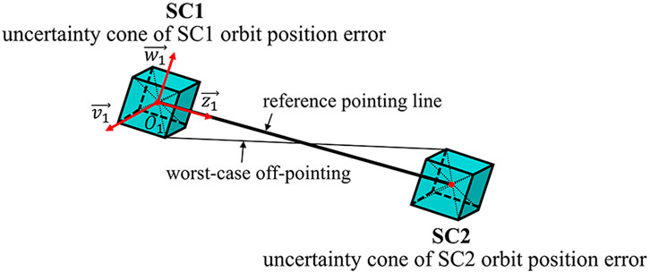
Figure 4. Uncertainty cone generated by the uncertainty of SC position in orbit determination in deep space.

Specifically, this uncertainty is characterized by the angle between the line connecting the two SCs. The following sections provide a detailed explanation of the calculation process (Cirillo and Gath, 2009). The unit position vector from SC1 to SC2 can be expressed by Equations 9, 10

${\vec{z}}_{1-2}=\frac{{\left[x_{12},y_{12},z_{12}\right]}^T}{L_{12,ref}},(9)$

with

$L_{12,ref}=\sqrt{x_{12}^2+y_{12}^2+z_{12}^2},(10)$

$\delta {\vec{L}}_{12,err}$ is the relative current position navigation error vector from SC1 to SC2.

$\delta {\vec{L}}_{12,err}={\left[\delta x_{12},\delta y_{12},\delta z_{12}\right]}^T.(11)$

the projection of the relative position navigation error vector from SC1 to SC2 in the direction of the relative position vector from SC1 to SC2 can be expressed as

$\delta {{\vec{L}}_{12,err}}^{\prime }=\delta L_{12}{\left[x_{12},y_{12},z_{12}\right]}^T,(12)$

with

$\delta L_{12}=\frac{\left[x_{12}\delta x_{12}+y_{12}\delta y_{12}+z_{12}\delta z_{12}\right]}{L_{12,ref}^2}.(13)$

$\delta \stackrel{⟶}{r_{12}}$ is the relative position navigation error along a coordinate axis of the inertial heliocentric frame provided by the DSN (estimated to be as 2 km).

$\begin{array}{ll}\hfill & \hfill \delta \stackrel{⟶}{r_{12}}=\delta {\vec{L}}_{12,err}-\delta {\vec{L}}_{12,err}^{\prime }\\ \hfill & ={\left[\delta x_{12}-\delta L_{12}{x}_{12},\delta y_{12}-\delta L_{12}{y}_{12},\delta z_{12}-\delta L_{12}{z}_{12}\right]}^T.\hfill \end{array}(14)$

$|\delta {\stackrel{⟶}{r}}_{12}|=\sqrt{{\left(\delta x_{12}-x_{12}\delta L_{12}\right)}^2+{\left(\delta y_{12}-y_{12}\delta L_{12}\right)}^2+{\left(\delta z_{12}-z_{12}\delta L_{12}\right)}^2}.(15)$

the uncertainty region contribution ${\theta }_u$ from the navigation error is given by the trigonometric equation:

$\begin{array}{ll}\hfill & \hfill {\theta }_{u,12}=\arcsin \left(\frac{|\stackrel{⟶}{\delta r_{12}}|}{L_{12,ref}-2|\stackrel{⟶}{\delta r_{12}}|}\right)\approx \frac{\sqrt{{\delta w}^2+{\delta v}^2}}{L_{12,ref}}\\ \hfill & =\frac{1}{\sqrt{L_{12,ref}^2}}\sqrt{{\left(\delta x_{12}-\delta L_{12}\cdot x_{12}\right)}^2+{\left(\delta y_{12}-\delta L_{12}\cdot y_{12}\right)}^2+{\left(\delta z_{12}-\delta L_{12}\cdot z_{12}\right)}^2},\hfill \end{array}(16)$

where $L_{12,ref}$ is the arm length without orbit position error. Equation 16 represents the worst-case navigation error and it is illustrated in Figure 4.

3 Acquisition strategy and capture process

3.1 The acquisition strategies

In our experimental setup for the scanning and acquisition strategy, we assume that ${\sigma }_{\mathit{yaw}}$ and ${\sigma }_{\mathit{pitch}}$ are independently distributed. When two SCs reach the target positions, through orbit determination by the DSN, their coordinates are located at any point within a tube of 2 km in diameter. The SC first needs to use a star tracker for attitude adjustment to complete the initial pointing in order to avoid a back - to - back configuration. Our acquisition and scanning strategy is applicable after the SC completes the initial pointing.

Successful acquisition occurs when the SC detector’s FOV and the laser spot both overlap the target area, enabling link establishment. Given the calculated effective detection range, the original CCD camera has been replaced by a QPD using DPS angle measurement technology. The QPD’s FOV is ${\theta }_{\text{FOV}}=1.43\text{\hspace{0.17em}mrad}$, and after being reduced by the telescope, it remains sufficient to fully cover the uncertainty region. Therefore, during the acquisition phase, the laser spot coverage on the remote SC alone serves as the criterion for successful acquisition.

Based on the angular size of the uncertainty region after filtering by the AEKF, distinct acquisition strategies have been developed. To facilitate the calculation of scanning time, the AEKF-filtered results are converted into polar coordinates. Using the angular position and radius $R$ in polar coordinates, we determine the path length required for a spiral trajectory to cover a specific point as shown in Figure 5. The main goal is to maximize the probability of successful link acquisition rather than to minimize the acquisition time. Once established, the laser link is intended to remain stable with minimal risk of disconnection. As a result, the scanning strategy focuses on thoroughly covering the uncertainty region to ensure reliable laser link capture.

Figure 5

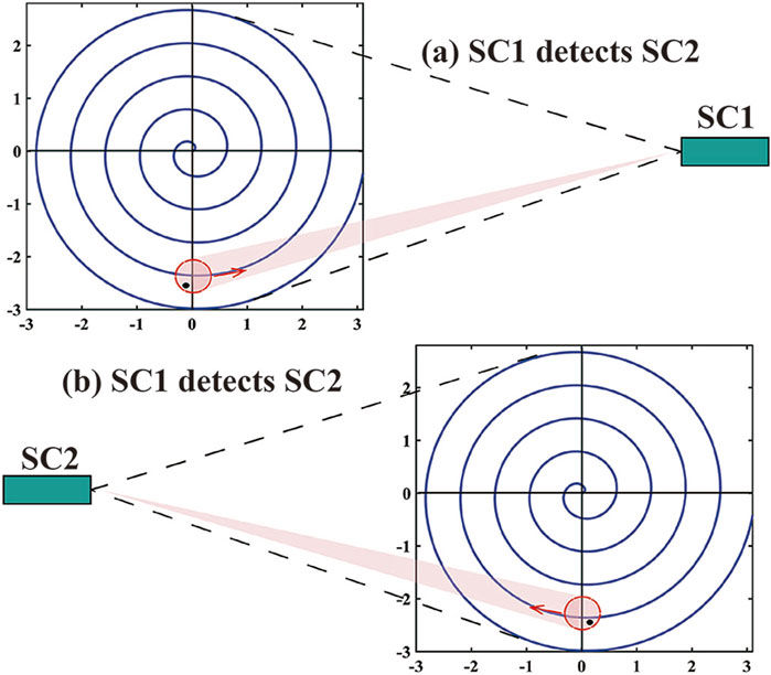
Figure 5. Schematic of the spacecraft scanning at both ends. In (a), SC1 detects SC2, shown with SC1 on the right performing spiral scanning of the uncertainty region. In (b), SC2 detects SC1, shown with SC2 on the left performing spiral scanning of the uncertainty region.

3.1.1 Strategy 1: scan by PAAM

When the uncertain cone angle $\theta$ is greater than the laser divergence angle ${\theta }_{\text{div}}$ but within the dynamic range of the optical angle ${\theta }_{\text{PAAM}}$ of the PAAM, this scheme relies solely on the rapid scanning capability of the PAAM. During the scanning process, the PAAM follows an Archimedean spiral path with uniform linear velocity.

3.1.2 Strategy 2: scanning strategy combining PAAM and micro-newton thrusters

When the uncertain cone angle $\theta$ exceeds the adjustment range of the PAAM optical angle ${\theta }_{\text{PAAM}}$, we need to expand the scanning range by combining SC attitude adjustments using micro-newton thrusters with PAAM scanning. In this scheme, both SC at the ends employ a scanning strategy that integrates discrete attitude adjustments via SC micro-newton thrusters with rapid and continuous scanning by the PAAM. The specific implementation process is as follows: The micro-newton thrusters perform discrete movements following an Archimedean spiral path with fixed step sizes and overlap ratios. For each discrete control maneuver of the micro-newton thrusters, the PAAM conducts a full-coverage scan along the Archimedean spiral path with a constant angular velocity, covering 90% of its maximum deflection range per revolution.

3.2 Search time

In the ATP phase of the gravitational waves detection in space, a primary focus is placed on enhancing the success probability of link establishment, with an emphasis on minimizing the time required for link establishment while ensuring full coverage scanning. The experimental configuration adopts a spiral scanning method, proven to be an efficient means of encompassing the entire uncertainty region. By setting the spiral line spacing equal to the diameter of the laser beam divergence angle, full coverage of the uncertain region can be achieved during uniform linear velocity scanning. The Archimedean spiral is parameterized as

$r=b\cdot \theta .(17)$

$\theta$ represents the polar angle, which increases by $2\pi$ for every complete rotation, and $r$ denotes the radius of the helix. The parameter $b$ defines the incremental change in the helical radius per full revolution, and its relationship with the trajectory width $D_t$ is given by: $D_t=2\pi b$. From (Equation 17), we can calculate the total length of the spiral by integrating along the spiral path. It is given by Equation 18

$L=\frac{1}{2}\left(r\sqrt{1+{\left(\frac{r}{b}\right)}^2}+b\cdot \text{arcsinh}\left(\frac{r}{b}\right)\right).(18)$

When scanning the uncertainty region by means of SC attitude adjustments, the scanning process can be regarded as a uniform angular velocity scanning in which the SC’s attitude is fine-tuned through micro-newton thruster adjustments and the SC’s scanning angular velocity is ${\omega }_{\text{micro}}=1\mu \text{rad/s}$. The scanning time $T_{micro}$ can be calculated using Equation 19

$T_{\mathit{micro}}=\frac{L}{{\omega }_{\text{micro}}}=\frac{1}{{\omega }_{\text{micro}}}\left(r\sqrt{1+{\left(\frac{r}{b}\right)}^2}+b\cdot \text{arcsinh}\left(\frac{r}{b}\right)\right).(19)$

The scanning process can be regarded as a uniform linear velocity when only the PAAM is used to scan the uncertainty region. Currently, the scanning angular velocity of the PAAM is approximately ${\omega }_{\text{PAAM}}=1\text{mrad/s}$. The scanning time $T_1$ can be calculated using Equation 20

$T1=\frac{L}{{\omega }_{\text{PAAM}}}=\frac{1}{{\omega }_{\text{PAAM}}}\left(r\sqrt{1+{\left(\frac{r}{b}\right)}^2}+b\cdot \text{arcsinh}\left(\frac{r}{b}\right)\right).(20)$

In the scanning scheme in which the PAAM is coordinated with SC attitude adjustments, the scanning process can be considered as a discrete motion. Moreover, by adjusting the scanning step size and overlap ratio, full coverage of uncertain areas is maintained. Concurrently, this is paired with the uniform angular velocity scanning strategy of PAAM, allowing the scanning time, $T_{PAAM}$, to be calculated using Equation 21

$T_{\text{PAAM}}=\frac{1}{{\omega }_{\text{PAAM}}}\left(r_{\text{PAAM}}\sqrt{1+{\left(\frac{r_{\text{PAAM}}}{b}\right)}^2}+b\cdot \text{arcsinh}\left(\frac{r_{\text{PAAM}}}{b}\right)\right),(21)$

where $r_{\text{PAAM}}$ is the maximum deflection angle of PAAM, $r_{\text{PAAM}}=6\mu rad$. The total scan time for fourth scheme be calculated using Equation 22

$T_2={\left(\frac{r}{r_{\text{PAAM}}\cdot p}\right)}^2\cdot T_{\text{PAAM}}+\left[{\left(\frac{r}{r_{\text{PAAM}}\cdot p}\right)}^2-1\right]\cdot \delta t,(22)$

where $p$ is the overlap rate in the discrete scanning process of SC attitude adjustment by micro-newton thrusters, $p=0.8$. $\delta t$ is the time needed to change the direction between adjacent spots.

3.3 The capture process

During the capture phase, the light received from the distant SC is weak, making it challenging for the local detector to observe the distant light spot when the local laser is active. Therefore, at the start of the scanning process, a toggling strategy is adopted: when the local laser is active, the remote receiving SC turns off its laser, and vice versa. That is, the local laser is turned off when the distant SC activates its laser for scanning. The inter-satellite link is established once the scientific QPD on each SC detects an interference signal. After the inter-satellite link is established and before scientific measurements begin, it is necessary to return PAAM to its original position by adjusting the SC’s attitude to avoid exceeding PAAM’s adjustment range during the scientific measurement phase. Specifically, within the detector’s field of view, as PAAM moves toward the zero position, the micro-newton thrusters adjust the SC’s attitude in the opposite direction. Throughout this adjustment, it is crucial to synchronize the speeds of PAAM and the micro-newton thrusters to prevent disruptions to the interference signal on the QPD.

4 Adaptive extended Kalman filter for ATP

In this section, we shall introduce the AEKF method, on the basis of which we develop a new control algorithm for the ATP phase. We will briefly describe the AKEF framework (Yang et al., 2024) and then apply it to the laser link acquisition in what follows.

4.1 Construction of an adaptive extended Kalman filter

Consider a hybrid extended Kalman filter in which the physical system concerned is governed by continuous and nonlinear dynamic equations, and the measurements are discrete in time as shown in Equation 23

$\left\{\begin{array}{c}{\displaystyle \dot{X}}=f\left(X,t\right)+w\left(t\right),\hfill \\ Z_k=h_k\left(X_k,v_k\right),\hfill \end{array}\right.(23)$

where both the dynamic function $f\left(X,t\right)$ and the measurement function $h_k\left(X_k\right)$ are nonlinear, $w(t)$ is the continuous noise. $w_k$ is the system noise and $v_k$ is the colored measurement noise as shown in Equation 24

$\left\{\begin{array}{c}E\left[w\left(t\right)w^T\left(t+\tau \right)\right]=Q_c\delta \left(t\right),\hfill \\ w_k\sim \left(0,Q_k\right),\hfill \\ Q_k=Q_c\left(k\mathrm{\Delta }t\right)/\mathrm{\Delta }t,\hfill \\ v_{k+1}={\mathrm{\Psi }}_{k,k-1}{v}_k+{\xi }_k.\hfill \end{array}\right.(24)$

We use Gaussian white noise as the system noise in this simulation, with the covariance matrix denoted as $Q_c$. At time $k$, the average $Q_k$ is computed from the continuous $Q_c$ over time $t$, and this averaged $Q_k$ serves as the covariance matrix of the process noise at time $k$. In the equations, ${\xi }_k$ denotes a white noise sequence with zero mean, and ${\mathrm{\Psi }}_{k,k-1}$ represents the coefficient transition matrix for the colored measurement noise.

In the AEKF, we can treat the measurement noise as a state quantity and include it in the state equation (Wang et al., 2014). The state equation of the Kalman filter, which includes the extended system noise and the measurement noise, may be written as Equation 25.

$\left[\begin{array}{c}\hfill X_{k+1}\hfill \\ \hfill v_{k+1}\hfill \end{array}\right]=\left[\begin{array}{cc}\hfill {\varphi }_{k,k-1}\hfill & \hfill 0\hfill \\ \hfill 0\hfill & \hfill {\mathrm{\Psi }}_{k,k-1}\hfill \end{array}\right]\left[\begin{array}{c}\hfill X_k\hfill \\ \hfill v_k\hfill \end{array}\right]+\left[\begin{array}{cc}\hfill {\mathrm{\Gamma }}_{k+1,k}\hfill & \hfill 0\hfill \\ \hfill 0\hfill & \hfill I\hfill \end{array}\right]\left[\begin{array}{c}\hfill W_k\hfill \\ \hfill {\xi }_k\hfill \end{array}\right],(25)$

where ${\mathrm{\Gamma }}_{k+1,k}$ is an identity matrix. The formula of EKF algorithm subject to the colored measurement noise can be referred to (Yang et al., 2024).

4.2 ATP control loop design

The AEKF method is an efficient predictive filtering approach that utilizes data from the previous step to predict the outcome of the next step. In a LISA-type mission, unlike the EKF considered before for clock synchronization purposes in the pre-TDI data post-processing (Wang et al., 2014), the AEKF for ATP will be carried out on orbit. Our design of the ATP control mainly includes the beam pointing control of PAAM and the control of the SC’s attitude by the micro-newton thruster. In the PAAM beam pointing control system, the FPGA control chip receives feedback signals from PAAM’s capacitance sensors. In the micro-newton thruster-based SC attitude control system, the thrusters regulate the SC’s attitude by using the feedback signals from STRs and the far-field spot position data of the target SC, which the QPD provides based on DPS angle measurement.

The ATP control system combines the information of the SC orbit integrator for feedforward control. Figure 6 shows the block diagram design of the control system of the ATP. In this control system, a theoretical model is established by AEKF and SC orbital integrator to control the PAAM. The output value controlled by the PID is weighted with the system noise as the state input to AEKF, and the measurement noise is added to simulate the actual situation on the SC. The whole control loop is closed-loop controlled by capacitance sensors, STRs, and a QPD based on DPS angle measurement technology. Taking into account the creep and hysteresis of piezoelectric ceramics in the PAAM, nonlinear compensation, and notching filters are added to the control loop to improve the stability of the whole control loop.

Figure 6

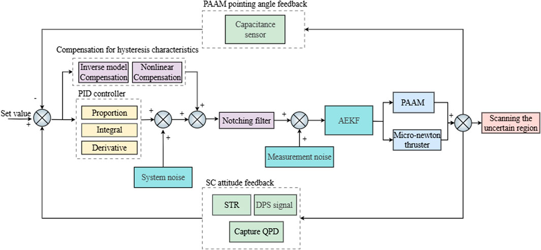
Figure 6. ATP control framework.

4.3 AEKF model for ATP

First, we define a 20-dimensional column state vector, which includes the position and velocity information of three SCs as shown in Equation 26 (Wang et al., 2014; Yang et al., 2024).

$x={\left[\stackrel{⟶}{x_1},\stackrel{⟶}{x_2},\stackrel{⟶}{x_3},\stackrel{⟶}{v_1},\stackrel{⟶}{v_2},\stackrel{⟶}{v_3},\stackrel{⟶}{\delta x_1},\stackrel{⟶}{\delta x_2},\stackrel{⟶}{\delta x_3},\stackrel{⟶}{\delta v_1},\stackrel{⟶}{\delta v_2},\stackrel{⟶}{\delta v_3}\right]}^T,(26)$

where $\overrightarrow{x_i}={(x_i,y_i,z_i)}^T$ are the SC positions, $\overrightarrow{v_i}={(v_{xi},v_{yi},v_{zi})}^T$ are the SC velocities, $\stackrel{⟶}{\delta x_i}={(\delta x_i,\delta y_i,\delta z_i)}^T$ and $\stackrel{⟶}{\delta v_i}={(\delta v_{xi},\delta v_{yi},\delta v_{zi})}^T$ are the position error and velocity error in SC orbit determination, and $i=1;2;3$ is the SC index.

The dynamics of a single SC is described by the Keplerian equation for planetary motion given by Equation 27

${\ddot{\stackrel{⃗}{x}}}_k={\displaystyle \sum _p}G{M}_p\frac{{\vec{x}}_k-{\vec{R}}_p}{{‖{\vec{x}}_k-{\vec{R}}_p‖}^3}.(27)$

where $\overrightarrow{X_k}$ is the position of a SC, $M_p$, ${\vec{R}}_p$ are the mass and the coordinates of the $p$th celestial body (the Sun and the planets) in the solar system, ${\vec{x}}_k-{\vec{R}}_p$ is a vector pointing from that SC to the $p$ th celestial body. Gravitational forces originated from the Sun and the major planets, including Mercury, Venus, Earth + Moon, Mars, Jupiter, Saturn, Uranus, and Neptune (Han et al., 2022) are considered.

The dynamic equations are given by Equations 28, 29

$\frac{d}{dt}\left[\begin{array}{c}\hfill {\vec{x}}_k\hfill \\ \hfill {\vec{v}}_k\hfill \end{array}\right]=f\left({\vec{x}}_k,{\vec{v}}_k\right)=\left[\begin{array}{c}\hfill {\vec{v}}_k\hfill \\ \hfill {\displaystyle \sum _p}G{M}_p\frac{{\vec{x}}_k-{\vec{R}}_p}{{‖{\vec{x}}_k-{\vec{R}}_p‖}^3}\hfill \end{array}\right].(28)$

$\frac{d}{dt}\left[\begin{array}{c}\hfill {\overrightarrow{\delta x}}_k\hfill \\ \hfill {\overrightarrow{\delta v}}_k\hfill \end{array}\right]=f\left({\overrightarrow{\delta x}}_k,{\overrightarrow{\delta v}}_k\right)=\left[\begin{array}{c}\hfill {\overrightarrow{\delta v}}_k\hfill \\ \hfill {\displaystyle \sum _p}G{M}_p\frac{{\overrightarrow{\delta x}}_k-{\vec{R}}_p}{{‖{\overrightarrow{\delta x}}_k-{\vec{R}}_p‖}^3}\hfill \end{array}\right].(29)$

Define $\alpha ={\left(\overrightarrow{x_k},\overrightarrow{v_k}\right)}^T$, then we can get Equation 30

$\varphi =\frac{\partial f}{\partial \alpha }=\left[\begin{array}{cc}\hfill O_3\hfill & \hfill I_3\hfill \\ \hfill A\hfill & \hfill O_3\hfill \end{array}\right].(30)$

here $O_3$ is the zero matrix, $I_3$ is the $3\times 3$ identity matrix, and the expression of the $3\times 3$ matrix A is given by Equation 31

$A=-{\displaystyle \sum _p}\frac{G{M}_p}{{‖{\vec{x}}_k-{\vec{R}}_p‖}^3}{I}_3+{\displaystyle \sum _p}\frac{3G{M}_p}{{‖{\vec{x}}_k-{\vec{R}}_p‖}^5}\left({\vec{x}}_k-{\vec{R}}_p\right){\left({\vec{x}}_k-{\vec{R}}_p\right)}^T.(31)$

For the entire system, the dynamic matrix $\varphi =\frac{\partial f}{\partial x}$ is $36\times 36$. We omit its explicit expression here, as it can be obtained in a straightforward way from the above formulae. In our work that follows, we simulate the PAA data for 10 days. Since the PAA changes very slowly with a 1-year periodicity, we set the sampling frequency of the AEKF to 1s. In the initial design process, we considered the influence of SC displacement, velocity, and acceleration on PAA, but in our subsequent simulation, we found that the relative acceleration of the SC was irrelevant to the PAA calculations.

Next, we present the two-dimensional measurement equation, which relates the positions and velocities of the three SCs to the yaw and pitch PAAs. In our scheme, the position error in navigation can be expressed by Equation 32

$z_k=h_k\left(x_k,v_k\right)=\left[\begin{array}{ccc}\hfill {\text{PAA}}_{\text{yaw,\hspace{0.17em}}12},\hfill & \hfill {\text{PAA}}_{\text{pitch,\hspace{0.17em}}12},\hfill & \hfill {\theta }_{\text{u,}12},\hfill \\ \hfill {\text{PAA}}_{\text{yaw,\hspace{0.17em}}21},\hfill & \hfill {\text{PAA}}_{\text{pitch,\hspace{0.17em}}21},\hfill & \hfill {\theta }_{\text{u,}21}\hfill \end{array}\right](32)$

where ${\text{PAA}}_{\text{\hspace{0.17em}pitch,ij}}$ and ${\text{PAA}}_{\text{\hspace{0.17em}yaw,ij}}$ are respectively the pitch and the yaw PAA between SCi and SCj. ${\theta }_{\text{U,ij}}$ is the uncertainty cone caused by worst-case navigation error between SCi and SCj. $v_k$ is the measurement nosie. $H_k$ is a $636$ dimensional observation matrix. We omit its explicit expression here, since it can be obtained straightforwardly from the formulae below. The element $H_k[i,j]$ in the matrix $H_k$ may be expressed by Equation 33

$H_k\left[i,j\right]=\frac{\partial z_k\left[i\right]}{\partial x_k\left[j\right]}.(33)$

As an example, the [1,1] component of $H_k$, with the step index $k$ omitted, may is provided by Equations 34–37

$\begin{array}{cc}\hfill H\left[\mathrm{1,1}\right]& =\frac{1}{{\left|{\vec{R}}_{t,12}\right|}^2\cdot {\left|{\vec{R}}_{t,13}\right|}^2\cdot {\left|{\vec{R}}_{r,12}\right|}^2}\hfill \\ \hfill & \left[\left({e_z}_x+\left(\left(z_{12}+V{z}_{12}\cdot \mathrm{\Delta }t\right)-\left(z_{13}+V{z}_{13}\cdot \mathrm{\Delta }t\right)\right)\cdot \left(y_{12}-V_{y_{12}}\cdot \mathrm{\Delta }t\right)\right.\right.\hfill \\ \hfill & \left.+\left(\left(y_{13}+V{y}_{13}\cdot \mathrm{\Delta }t\right)-\left(y_{12}+V{y}_{12}\cdot \mathrm{\Delta }t\right)\right)\cdot \left(z_{12}-V_{z_{12}}\cdot \mathrm{\Delta }t\right)\right)\hfill \\ \hfill & \cdot \left|{\vec{R}}_{t,12}\right|\cdot \left|{\vec{R}}_{t,13}\right|\cdot \left|{\vec{R}}_{r,12}\right|\hfill \\ \hfill & -\left({e_z}_x\cdot \left(x_{12}-V_{x_{12}}\cdot \mathrm{\Delta }t\right)+{e_z}_y\cdot \left(y_{12}-V_{y_{12}}\cdot \mathrm{\Delta }t\right)+{e_z}_z\cdot \left(z_{12}-V_{z_{12}}\cdot \mathrm{\Delta }t\right)\right)\hfill \\ \hfill & \cdot \left(\left|{\vec{R}}_{t,13}\right|\cdot \left|{\vec{R}}_{r,12}\right|\cdot \frac{\partial \left|{\vec{R}}_{t,12}\right|}{\partial X_1}+\left|{\vec{R}}_{t,12}\right|\cdot \left|{\vec{R}}_{r,12}\right|\cdot \frac{\partial \left|{\vec{R}}_{t,13}\right|}{\partial X_1}\right.\hfill \\ \hfill & \left.\left.+\left|{\vec{R}}_{t,12}\right|\cdot \left|{\vec{R}}_{t,13}\right|\cdot \frac{\partial \left|{\vec{R}}_{r,12}\right|}{\partial X_1}\right)\right]\hfill \end{array}(34)$

with

$\frac{\partial \left|{\vec{R}}_{t,12}\right|}{\partial X_1}=\frac{2\left(x_{12}+V_{x_{12}}\mathrm{\Delta }t\right)}{2\left|{\vec{R}}_{t,12}\right|}=\frac{\left(x_{12}+V_{x_{12}}\mathrm{\Delta }t\right)}{\left|{\vec{R}}_{t,12}\right|}(35)$

$\frac{\partial \left|{\vec{R}}_{r,12}\right|}{\partial X_1}=\frac{2\left(x_{12}-V_{x_{12}}\mathrm{\Delta }t\right)}{2\left|{\vec{R}}_{r,12}\right|}=\frac{\left(x_{12}-V_{x_{12}}\mathrm{\Delta }t\right)}{\left|{\vec{R}}_{r,12}\right|}(36)$

$\frac{\partial \left|{\vec{R}}_{t,13}\right|}{\partial X_1}=\frac{2\left(x_{13}+V_{x_{13}}\mathrm{\Delta }t\right)}{2\left|{\vec{R}}_{t,13}\right|}=\frac{\left(x_{13}+V_{x_{13}}\mathrm{\Delta }t\right)}{\left|{\vec{R}}_{t,13}\right|}(37)$

In standard practice, the coefficient transfer matrix ${\mathrm{\Psi }}_{k,k-1}$ of colored measurement noise is determined by the ARMA model. In the present context, the definition of ${\mathrm{\Psi }}_{k,k-1}$ is relatively simple and can be considered as a special case of the ARMA model in which the autoregressive parameter is 1, and the moving average parameter is 0 (Fattah et al., 2011). We have also tried to use a more sophisticated ARMA model to estimate the value of the ${\mathrm{\Psi }}_{k,k-1}$ matrix, but the results are not as good as the methods used here. As shown in the state equation of AEKF, we only consider the colored noise component in the measurement noise and do not include white noise. Therefore, the ${\xi }_k$ term can be directly ignored. As shown in Equation 38, we approximately take the ratio of the measurement noise amplitudes at the previous moment and the current moment as input to the coefficient transfer matrix ${\mathrm{\Psi }}_{k,k-1}$ of the colored measurement noise. The simple choice here is likely due to a very slow variation of the colored measurement noise in the time domain at the annual level. This colored measurement noise is a linear superposition of all the colored noise types that we will discuss in detail shortly.

${\mathrm{\Psi }}_{k,k-1}=v_k/v_{k-1}.(38)$

In a standard AEKF, the size of the $Q_k$ and $R_k$ matrix is automatically adjusted by observing the prediction error and its mean square error matrix and introducing the fading factor to obtain a good estimation state (Li and Kennel, 2020). The AEKF designed in this paper is slightly different from the traditional AEKF. In the AEKF designed by us, the covariance matrix of measurement noise $R_k$ is updated in real-time according to the magnitude of measurement noise, while the covariance matrix of system noise $Q_k$ is updated every month or so, based on the accuracy of orbit prediction.

In this study, the flowchart for ATP based on AEKF is illustrated in Figure 7. During the first step of data preprocessing, we rely on orbit prediction to acquire the SC’s position and velocity information. The system noise data is linearly superimposed onto the orbit prediction data to form the system data. The orbit prediction data, linearly superimposed with the Grace-follow-on orbit STR noise data, constitutes the measurement data input into the AEKF. In the second step, during the AEKF process, the orbit prediction information needs to be updated weekly. Through the filtering results of AEKF, we can calculate the size of the initial uncertain region. Finally, by considering the scanning speeds of PAAM and micro-newton thrusters, we calculated the average scanning time for single-field full coverage under the two scanning strategies and conducted statistical analysis on the experimental results at the same time.

Figure 7

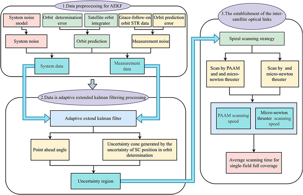
Figure 7. ATP flow chart based on AEKF.

4.4 Noise model

4.4.1 System noise model

To develop a system model for the AEKF, we established a system noise model specific to the ATP phase. This noise model primarily accounts for solar radiation pressure noise, noise induced by SC attitude jitter, and dynamic actuation errors of the PAAM. We imposed a total position error of $2\text{\hspace{0.17em}km}$ and a velocity error of $0.2\text{\hspace{0.17em}cm/s}$ on the SC as system noise. These position and velocity errors are incorporated as the initial state inputs to the orbital integrator in the AEKF, thereby constructing the system model for the filter. Furthermore, the covariance matrix $Q_k$ is configured based on the intensity of the system noise.

4.4.2 Measurement noise model

This section focuses on the ATP noise model, which serves as the basis for quantifying measurement noise in our subsequent simulations. During the simulation, we generate orbital prediction data by linearly superimposing the SC’s position and velocity outputs from the orbital integrator with orbit determination errors modeled as random noise. This resulting data is regarded as the true state for the AEKF. Measurement noise is then linearly added to this true state to produce the simulated measurements used as inputs for the AEKF. Meanwhile, the covariance matrix $R_k$, which characterizes the measurement noise within the AEKF, is dynamically calculated based on the generated noise and updated in real time, as shown in Equation 39.

$R_k=cov\left(v_k\right)=E\left\{v_k{v_k}^T\right\}.(39)$

The measurement noise model consists of two main components: the noise model for the PAA measurements and the noise model for ${\theta }_{\text{u}}$. The PAA measurement noise model is primarily derived through amplitude transformations based on on-orbit data from the GRACE Follow-On mission. In contrast, the measurement noise model for ${\theta }_{\text{u}}$ employs white noise to simulate orbital prediction errors. This chapter provides a detailed description of each of these models.

4.4.2.1 PAA measurement noise model

The measurement noise model for PAA accounts for various sources and mainly includes piston noise of PAAM, SC attitude jitter noise, laser intensity noise, laser shot noise, STR read-out noise, detector equivalent input current noise and other optical platform noises. During the ATP phase, the readout noise of the STR is the primary source of measurement noise. In our simulation, a STR with $1\times 10^{-5}$ rad readout noise was selected. To ensure that our simulation closely mirrors the actual conditions in orbit, we applied amplitude transformation to the STR measurement data from Grace-Follow-on mission, using it as the input for the measurement noise model.

First, we need to convert the STR quaternion data into the Euler angles representing the telescope’s vector direction. The attitude of the SC body relative to the ground inertial coordinate system is defined by the attitude quaternion. The attitude quaternion $q_{ib}\in R^{4\times 1}$ is represented as $q_{ib}={\left[q_{ib,0},q_{ib,1},q_{ib,2},q_{ib,3}\right]}^T$. To convert the four-element attitude data of the STR into the direction of the telescope vector, the four-element data must be converted into the rotation matrix $R_T$ (Vidano et al., 2020).

As shown in Figure 8, there is a 30° angle between the STR position vector and the telescope exit direction vector, so the STR position vector must be rotated 30° around the Z-axis. If the STR vector direction is expressed as ${[100]}^T$, then the telescope exit direction vector can be provided by Equation 40

$\begin{array}{ll}\hfill & \hfill \left[\begin{array}{c}\hfill {\alpha }_{ij}\hfill \\ \hfill {\beta }_{ij}\hfill \\ \hfill {\gamma }_{ij}\hfill \end{array}\right]=\left[\begin{array}{c}\hfill 1\hfill \\ \hfill 0\hfill \\ \hfill 0\hfill \end{array}\right]\ast \left[\begin{array}{ccc}\hfill \cos \left(\frac{\pi }{6}\right)\hfill & \hfill \sin \left(\frac{\pi }{6}\right)\hfill & \hfill 0\hfill \\ \hfill -\sin \left(\frac{\pi }{6}\right)\hfill & \hfill \cos \left(\frac{\pi }{6}\right)\hfill & \hfill 0\hfill \\ \hfill 0\hfill & \hfill 0\hfill & \hfill 1\hfill \end{array}\right]\ast R_T\\ \hfill & =\left[\begin{array}{c}\hfill \left(\sqrt{3}\left({q_{ib,0}}^2+{q_{ib,1}}^2\right)-\sqrt{3}/2\right)+\left(-q_{ib,0}{\ast q}_{ib,3}+q_{ib,1}{\ast q}_{ib,2}\right)\hfill \\ \hfill \sqrt{3}\left(q_{ib,0}{\ast q}_{ib,3}+q_{ib,1}{\ast q}_{ib,2}\right)+\left(\left({q_{ib,0}}^2+{q_{ib,2}}^2\right)-1/2\right)\hfill \\ \hfill \sqrt{3}\left({-q}_{ib,0}{\ast q}_{ib,2}+q_{ib,1}{\ast q}_{ib,3}\right)+\left(q_{ib,0}{\ast q}_{ib,1}+q_{ib,2}{\ast q}_{ib,3}\right)\hfill \end{array}\right].\hfill & \hfill & \hfill \end{array}(40)$

Figure 8

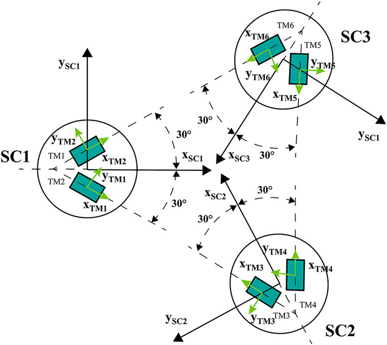
Figure 8. Spacecraft coordinates and telescope coordinates.

The error introduced during the conversion of STR quaternion data to the Euler angles representing the telescope’s vector direction ranges from $10^{-19}\text{\hspace{0.17em}rad}$ to $10^{-9}\text{\hspace{0.17em}rad}$ (Vidano et al., 2020). This level of accuracy is sufficient to meet our requirements. From this, we can derive the conversion relationship between the telescope vector and the STR quaternion data.

Subsequently, by applying amplitude variations to the time-domain noise data, we obtain time-domain PAA measurement noise data with average amplitudes of $1\times 10^{-5}\text{rad}$, as shown in Figure 9.

Figure 9

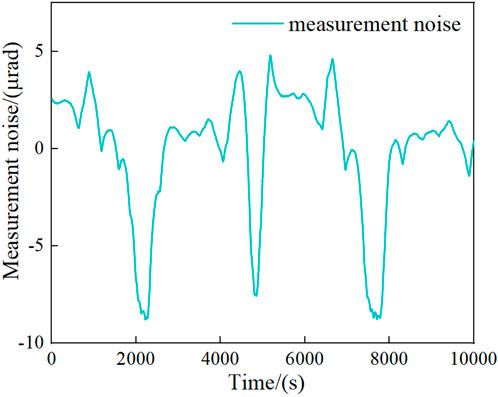
Figure 9. Measuremnet noise.

4.4.2.2 θ_u measurement noise model

To work out a ${\theta }_{\text{u}}$ measurement model for AEKF, consider

$\left\{\begin{array}{cc}\hfill & \delta X={\left[\delta X_i,\delta Y_i,\delta Z_i\right]}^T,\hfill \\ \hfill & \delta V={\left[\delta V_{Xi},\delta V_{Yi},\delta V_{Zi}\right]}^T,\hfill \end{array}\right.(41)$

here, $\delta X$ and $\delta V$ denote the position and velocity errors in orbit prediction as shown in Equation 41. The SC’s position and velocity from the orbit integrator serve as AEKF inputs, with prediction errors treated as measurement noise. Equations 11–16 are then used to determine the uncertainty region caused by navigation errors.

Based on the orbital prediction experience from Tianwen-I, when a 24-h orbit determination is conducted using the DSN, the velocity determination error is $0.2\text{\hspace{0.17em}cm/s}$, and the position determination error is $200\text{\hspace{0.17em}m}$. Under these conditions, the establishment of the inter-satellite optical link can be achieved without relying on AEKF. However, from the viewpoint of autonomous navigation, it is feasible to use orbit prediction data for a month in the measurement model of the AEKF, provided the required precision in orbit determination on the position and velocity of the SC in orbit are respectively within the margins of 50km and 2 cm/s. This uncertainty region is input as the source of measurement noise for ${\theta }_{\text{u}}$, resulting in an error margin of approximately $10\mu \text{rad}$. We can also update the orbit determination error by ground tracking during data transmission between the SC and the ground station. Our proposed scheme is primarily designed for scenarios with lower orbit determination accuracy. The measurement noise of ${\theta }_{\text{u}}$ is added to the actual ${\theta }_{\text{u}}$ value provided by the orbital integrator in the form of white noise.

5 Results and discussion

In this section, we conduct an error analysis on the results of PAA and ${\theta }_{\text{u}}$ after AEKF filtering. Additionally, based on the filtered results, we linearly superimpose the installation error and measurement noise of the STR. This allows us to investigate the single-field scan time changes under different scanning strategies before and after AEKF filtering.

5.1 AEKF result analysis

We simulated measurements of about 10,000 s with a sampling frequency of 1 Hz. Only the laser link between two of the three SCs was considered for analysis in this simulation. Figure 10 shows the AEKF prediction results of the PAA between SC1 and SC2. Before AEKF filtering, the average PAA error between SC1 and SC2 was 9 $\mu$rad. After AEKF filtering, the maximum AEKF prediction error of SC1 relative to SC2 in the pitch direction is $1.1\text{nrad}$, and the maximum AEKF prediction error of SC1 relative to SC2 in the yaw direction is $1.2\text{nrad}$. The maximum AEKF prediction error of SC2 relative to SC1 in the pitch direction is $1.01\text{nrad}$, and the maximum AEKF prediction error of SC2 relative to SC1 in the yaw direction is $1.21\text{nrad}$.

Figure 10

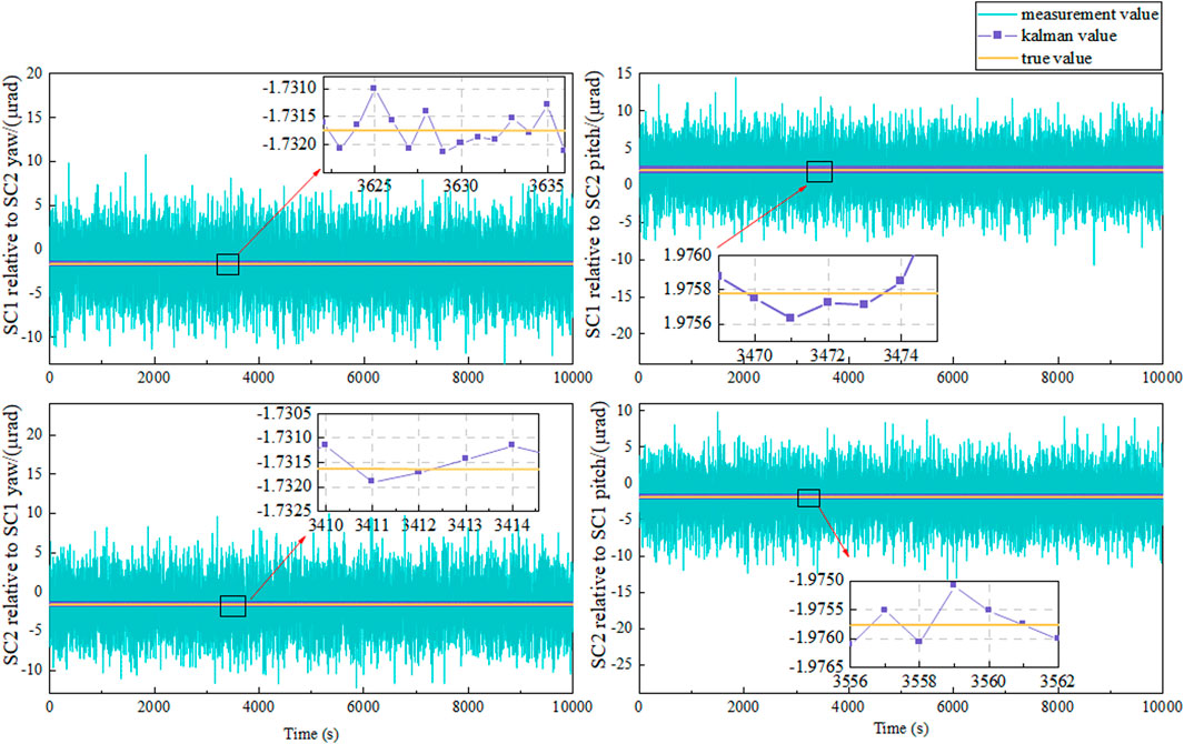
Figure 10. The AEKF prediction results of PAA between SC1 and SC2.

Figure 11 shows the AEKF prediction errors of the PAA between SC1 and SC2. The average prediction error of the AEKF from SC1 relative to SC2 in the pitch direction is $0.69\text{nrad}$, and the average prediction error of the AEKF from SC1 relative to SC2 in the yaw direction is $0.67\text{nrad}$. The average prediction error of the AEKF from SC2 relative to SC1 in the pitch direction is $0.67\text{nrad}$, and the average prediction error from SC2 relative to SC1 in the yaw direction is $0.76\text{nrad}$. The AEKF filtering effectively decreased the average PAA error of SC1 relative to SC2 by 82.31 dB in the pitch direction and 82.56 dB in the yaw direction. In contrast, the average navigation error of SC2 relative to SC1 was reduced by 82.56 dB in the pitch direction and 81.47 dB in the yaw direction.

Figure 11

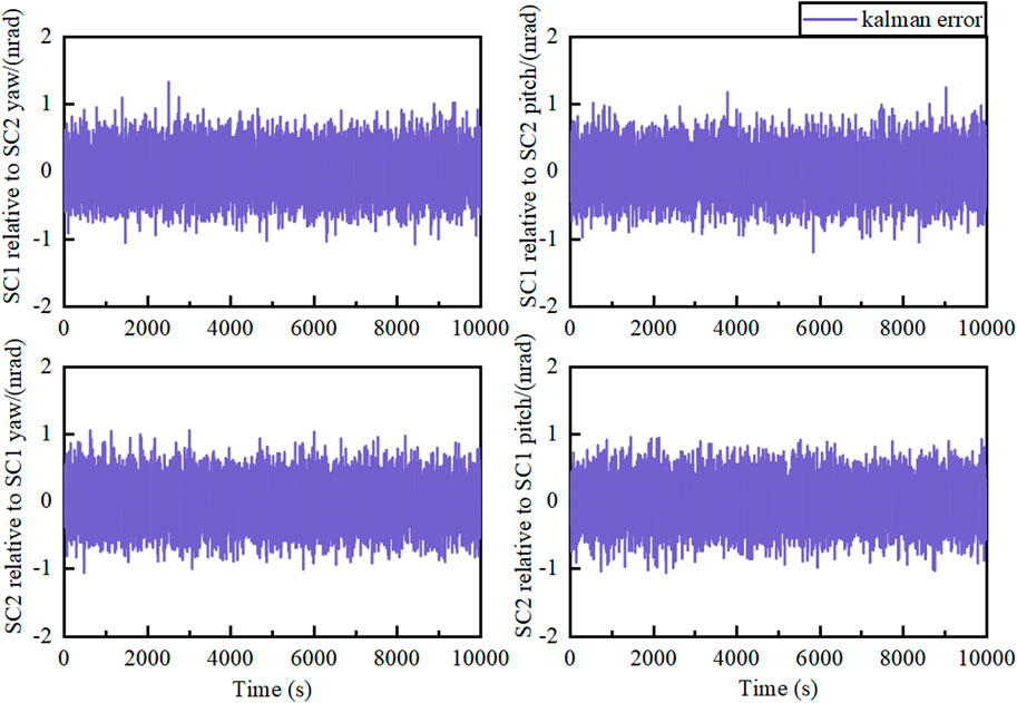
Figure 11. The AEKF prediction errors of PAA between SC1 and SC2.

Figure 12 presents the prediction results of the navigation error between SC1 and SC2 using the AEKF during the scanning process. Before AEKF filtering, the average navigation error of SC1 relative to SC2 was 9 $\mu$rad. After AEKF filtering, the maximum navigation error of SC1 relative to SC2 decreased to 0.27 $\mu$rad, with an average navigation error of 0.1 $\mu$rad. Similarly, before AEKF filtering, the average navigation error of SC2 relative to SC1 was 10 $\mu$rad, which was reduced to a maximum of 0.23 $\mu$rad and an average of 0.16 $\mu$rad after filtering. The AEKF filtering effectively decreased the average navigation error of SC1 relative to SC2 by 39.08 dB, while the average navigation error of SC2 relative to SC1 was reduced by 35 dB.

Figure 12

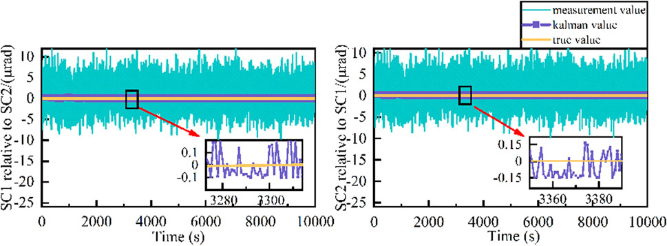
Figure 12. ${\theta }_{\text{u}}$ AEKF prediction results.

Table 1 provides a summary of the maximum and average total noise levels under colored measurement noise conditions, as well as the maximum and average prediction errors for PAA and ${\theta }_{\text{u}}$ using the AEKF. The results presented in Table 1 indicate that the AEKF significantly suppresses noise under colored measurement noise conditions. Additionally, noise suppression is more effective in the pitch direction than the yaw direction. This difference is likely due to the PAA having a smaller pitch adjustment range than the yaw direction, leading to a smoother variation process that enables the AEKF to achieve more effective noise suppression.

Table 1

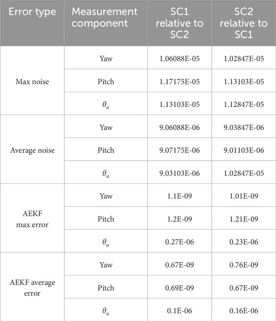
Table 1. AEKF errors between SC1 and SC2.

In our simulation, the orbital dynamics and updates to the SC’s state of motion are incorporated into the iterations of the AEKF. Table 2 summarizes the results of the maximum prediction errors for the pitch PAA and yaw PAA between the two SCs, both before and after filtering.

Table 2

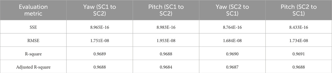
Table 2. Fitting result.

Figure 13 shows the histogram of the pitch and yaw error distribution for SC1 relative to SC2 and SC2 relative to SC1, both before and after AEKF filtering. The AEKF effectively reduces the pitch and yaw errors of SC1 relative to SC2 and SC2 relative to SC1, thereby decreasing the size of the initial uncertainty region during the ATP phase. Furthermore, the AEKF has a more pronounced effect on reducing the RMS of the pitch and yaw direction errors.

Figure 13

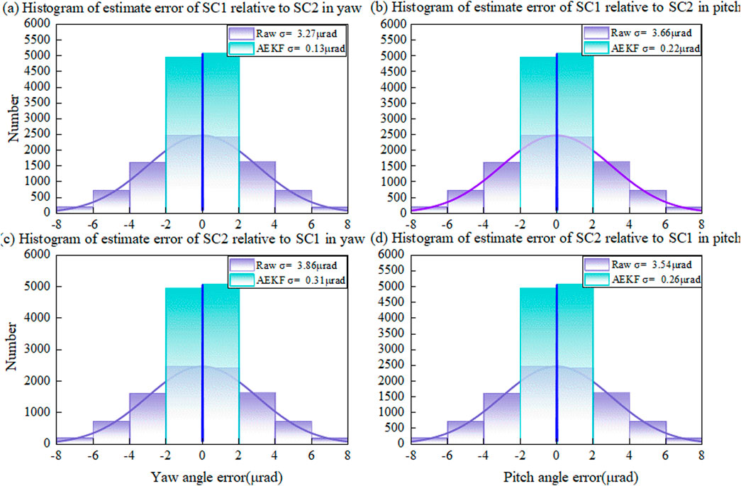
Figure 13. Histogram of the pitch and yaw error distribution between SC1 and SC2 before and after AEKF filtering. (a) Histogram of the estimate error of SC1 relative to SC2 in yaw direction. (b) Histogram of the estimate error of SC1 relative to SC2 in pitch direction. (c) Histogram of the estimate error of SC2 relative to SC1 in yaw direction. (d) Histogram of the estimate error of SC2 relative to SC1 in pitch direction.

5.2 Comparison of single-field full coverage scanning results

Figure 14 shows the cumulative probability curves and probability density curves before and after the application of AEKF under different scanning strategies. The results demonstrate that the scanning method integrating PAAM scanning with SC attitude adjustment can save more scanning time than the method that solely relies on SC attitude adjustment. Meanwhile, under different scanning strategies, AEKF filtering is effective in reducing the scanning time.

Figure 14

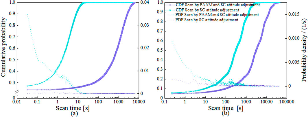
Figure 14. (a) Cumulative probability curves and probability density curves against the scanning time after the application of AEKF. (b) Cumulative probability curves and probability density curves against the scanning time before the application of AEKF.

Table 3 summarizes the average scanning time, both before and after AEKF filtering, required for single-field full coverage. The comparison includes two types of scenarios. One scenario involves scanning using a combination of the PAAM and micro-newton thrusters, while the other relies solely on micro-newton thrusters. The results indicate that AEKF filtering effectively reduces the time needed for full coverage scanning. Furthermore, employing the PAAM in conjunction with micro-newton thrusters significantly enhances the efficiency of the link-establishment process. As a result, it dramatically reduces the overall link acquisition time compared to the traditional strategy that relies solely on micro-newton thrusters.

Table 3

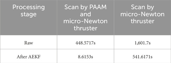
Table 3. Average scanning time comparison before and after AEKF filtering.

6 Concluding remarks

Our work presents a new laser link acquisition scheme in the detection of gravitational waves in space. In place of the CCD camera in the conventional scheme, an AEKF is incorporated into the control loop of the PAAM to steer a laser beam in such a way to reduce the uncertainty cone in the initial acquisition. This scheme relies on high-precision orbit determination data as the initial input, ensuring the effectiveness of the AEKF. In addition, it avoids the heating and ventilation problems associated with CCD cameras and simplifies spacecraft payload design. The proposed scheme also merges the coarse and fine acquisition processes of the conventional method into a single step, thereby improving acquisition efficiency and reducing operational time. Numerical simulations in scenarios closely resemble the prospective on orbit situations further verify the feasibility of this scheme.

Currently, we are setting up a tabletop experiment to validate the AEKF constructed in the hardware setup. In addition, we are also looking at the feasibility to enlarge the dynamic range of the PAAM so as to replace micro-newton thruster scanning functions entirely during the ATP phase. More experimental results will be reported soon. It is also expected that the new scheme will provide new alternatives for establishing laser link in future inter-satellite laser communication systems in deep space.

Data availability statement

All data that support the findings of this study are included within the article (and any supplementary files).

Author contributions

JY: Data curation, Formal Analysis, Methodology, Writing – original draft, Writing – review and editing. YX: Formal Analysis, Writing – review and editing. YF: Methodology, Writing – review and editing. PW: Conceptualization, Methodology, Software, Writing – review and editing. XW: Formal Analysis, Investigation, Supervision, Writing – review and editing. ZC: Methodology, Software, Writing – review and editing. JJ: Resources, Software, Writing – review and editing. YT: Software, Investigation, Writing – review and editing. YL: Data curation, Methodology, Writing – original draft, Writing – review and editing.

Funding

The author(s) declare that financial support was received for the research and/or publication of this article. This work is supported by the National Key R&D Program of China (2022YFC2203701).

Acknowledgments

Our thanks to the hard-working editors and for valuable comments from the reviewers.

Conflict of interest

The authors declare that the research was conducted in the absence of any commercial or financial relationships that could be construed as a potential conflict of interest.

Generative AI statement

The author(s) declare that no Generative AI was used in the creation of this manuscript.

Any alternative text (alt text) provided alongside figures in this article has been generated by Frontiers with the support of artificial intelligence and reasonable efforts have been made to ensure accuracy, including review by the authors wherever possible. If you identify any issues, please contact us.

Publisher’s note

All claims expressed in this article are solely those of the authors and do not necessarily represent those of their affiliated organizations, or those of the publisher, the editors and the reviewers. Any product that may be evaluated in this article, or claim that may be made by its manufacturer, is not guaranteed or endorsed by the publisher.

References

Ales, F., Gath, P. F., Johann, U., and Braxmaier, C. (2014). Modeling and simulation of a laser ranging interferometer acquisition and guidance algorithm. J. Spacecr. Rockets 51, 226–238. doi:10.2514/1.a32567

CrossRef Full Text | Google Scholar

Cirillo, F., and Gath, P. F. (2009). Control system design for the constellation acquisition phase of the lisa mission. J. Phys. Conf. Ser. 154, 012014. doi:10.1088/1742-6596/154/1/012014

CrossRef Full Text | Google Scholar

Cui, B., Zhao, G., Xia, Y., Wang, P., and Zhang, Y. (2024). A variable-bandwidth extended state observer for nonlinear systems with measurement noise. IEEE Trans. Industrial Electron. 72, 1946–1957. doi:10.1109/tie.2024.3419254

CrossRef Full Text | Google Scholar

Danzmann, K.the LISA Study Team (1996). LISA: laser interferometer space antenna for gravitational wave measurements. Class. Quantum Gravity 13, A247–A250. doi:10.1088/0264-9381/13/11A/033

CrossRef Full Text | Google Scholar

Fattah, S., Zhu, W.-P., and Ahmad, M. (2011). Identification of autoregressive moving average systems based on noise compensation in the correlation domain. IET signal Process. 5, 292–305. doi:10.1049/iet-spr.2009.0240

CrossRef Full Text | Google Scholar

Gao, R., Liu, H., Zhao, Y., Luo, Z., and Jin, G. (2021a). Automatic, high-speed, high-precision acquisition scheme with QPD for the Taiji program. Opt. Express 29, 821–836. doi:10.1364/oe.408822

PubMed Abstract | CrossRef Full Text | Google Scholar

Gao, R., Liu, H., Zhao, Y., Luo, Z., Shen, J., and Jin, G. (2021b). Laser acquisition experimental demonstration for space gravitational wave detection missions. Opt. Express 29, 6368–6383. doi:10.1364/oe.414741

PubMed Abstract | CrossRef Full Text | Google Scholar

Han, X., Peng, X., Tang, W., Yang, Z., Ma, X., Gao, C., et al. (2022). Effect of celestial body gravity on Taiji mission range and range acceleration noise. Phys. Rev. D. 106, 102005. doi:10.1103/physrevd.106.102005

CrossRef Full Text | Google Scholar

Hechenblaikner, G., Delchambre, S., and Ziegler, T. (2023). Optical link acquisition for the lisa mission with in-field pointing architecture. Opt. and Laser Technol. 161, 109213. doi:10.1016/j.optlastec.2023.109213

CrossRef Full Text | Google Scholar

Hu, Q.-L., Zhang, J.-Y., Nie, R.-L., Yang, M.-L., Cao, B., Jiao, X.-X., et al. (2024). Ground-based simulation of laser link acquisition for inter-satellite laser interferometry. Opt. Express 32, 31006–31022. doi:10.1364/OE.530639

PubMed Abstract | CrossRef Full Text | Google Scholar

Li, X., and Kennel, R. (2020). General formulation of kalman-filter-based online parameter identification methods for vsi-fed pmsm. IEEE Trans. Industrial Electron. 68, 2856–2864. doi:10.1109/tie.2020.2977568

CrossRef Full Text | Google Scholar

Li, Z., and Zheng, J. (2021). Orbit determination for a space-based gravitational wave observatory. Acta Astronaut. 185, 170–178. doi:10.1016/j.actaastro.2021.04.014

CrossRef Full Text | Google Scholar

Liu, H., Niu, X., Zeng, M., Wang, S., Cui, K., and Yu, D. (2022). Review of micro propulsion technology for space gravitational waves detection. Acta astronaut. 193, 496–510. doi:10.1016/j.actaastro.2022.01.043

CrossRef Full Text | Google Scholar

Luo, J., Chen, L.-S., Duan, H.-Z., Gong, Y.-G., Hu, S., Ji, J., et al. (2016). TianQin: a space-borne gravitational wave detector. Class. Quantum Gravity 33, 035010. doi:10.1088/0264-9381/33/3/035010

CrossRef Full Text | Google Scholar

Luo, Z., Wang, Q., Mahrdt, C., Goerth, A., and Heinzel, G. (2017). Possible alternative acquisition scheme for the gravity recovery and climate experiment follow-on-type mission. Appl. Opt. 56, 1495–1500. doi:10.1364/ao.56.001495

CrossRef Full Text | Google Scholar

Luo, Z., Guo, Z., Jin, G., Wu, Y., and Hu, W. (2020). A brief analysis to Taiji: science and technology. Results Phys. 16, 102918. doi:10.1016/j.rinp.2019.102918

CrossRef Full Text | Google Scholar

Miao, Y., Jian-cong, L., Hong-an, L., Yao-zhang, H., Jia-xiong, L., Yan-xiong, W., et al. (2023). Design of optical system for low-sensitivity space gravitational wave telescope. Chin. Opt. 16, 1384–1393. doi:10.37188/CO.2023-0006

CrossRef Full Text | Google Scholar

Vidano, S., Novara, C., Colangelo, L., and Grzymisch, J. (2020). The lisa dfacs: a nonlinear model for the spacecraft dynamics. Aerosp. Sci. Technol. 107, 106313. doi:10.1016/j.ast.2020.106313

CrossRef Full Text | Google Scholar

Vinet, J.-Y., Christensen, N., Dinu-Jaeger, N., Lintz, M., Man, N., and Pichot, M. (2019). LISA telescope: phase noise due to pointing jitter. Class. Quantum Gravity 36, 205003. doi:10.1088/1361-6382/ab3a16

CrossRef Full Text | Google Scholar

Wang, Y., Heinzel, G., and Danzmann, K. (2014). First stage of LISA data processing: clock synchronization and arm-length determination via a hybrid-extended Kalman filter. Phys. Rev. D. 90 (APS), 064016. doi:10.1103/physrevd.90.064016

CrossRef Full Text | Google Scholar

Wu, Y., Hai, H., Fang, S., Fan, W., Song, J., Zhao, K., et al. (2023). A fast steering mirror with ultra-low geometric tilt-to-length coupling noise for space-borne gravitational wave detection. Meas. Sci. Technol. 35, 015407. doi:10.1088/1361-6501/ad0317

CrossRef Full Text | Google Scholar

Yang, P., Huang, Y., Li, P., Wang, H., Fan, M., Liu, S., et al. (2022). Orbit determination of China’s first mars probe Tianwen-1 during interplanetary cruise. Adv. Space Res. 69, 1060–1071. doi:10.1016/j.asr.2021.10.046

CrossRef Full Text | Google Scholar

Yang, J., Xie, Y., Tang, W., Liang, X., Zhang, L., Cui, Z., et al. (2024). Adaptive extended kalman filter and point ahead angle prediction in the detection of gravitational waves in space. Phys. Rev. D. 110, 102007. doi:10.1103/PhysRevD.110.102007

CrossRef Full Text | Google Scholar

Yu, M., Huang, L., Liu, Y., Zou, D., Lin, H.-a., Li, J., et al. (2024). Simulation alignment of optical system for space gravitational wave telescope. Meas. Sci. Technol. 35, 066004. doi:10.1088/1361-6501/ad2cdc

CrossRef Full Text | Google Scholar

Zhu, W., Xie, Y., Qian, Y., Jia, J., Zhang, L., and Wang, X. (2024). Development and analysis of two-dimensional point-ahead angle mechanism for space gravitational-wave detection. Rev. Sci. Instrum. 95, 025002. doi:10.1063/5.0186061

PubMed Abstract | CrossRef Full Text | Google Scholar