Spacecraft radio signal polarization calibration

Introduction: The only reliable method to remotely obtain magnetic field information across large swaths of interplanetary/interstellar plasma is with the measurement of Faraday rotation of polarized radio signals.

Methods: Focusing on the high frequency regime of magnetized plasmas, this paper discusses the most difficult first step toward obtaining these measurements. Transitioning from raw voltage samples to plane of polarization measurements requires both simulated signal tests and qualitative inspections of the behavior of the resulting measurements.

Results: To demonstrate how this calibration approach works, we show examples collected from the STEREO A and B spacecraft and the Mars Reconnaissance Orbiter spacecraft.

Discussion: While astronomical radio sources have their own challenges to data processing, we show that spacecraft data have their own unique characteristics that can benefit and hinder the data processing.

1 Introduction

The properties of radio signals are modified by propagating through plasma. Inherently, all the modification is in phase and power which manifests as changes in properties of observed frequency, polarization, and intensity (Kraus, 1973). A radio antenna capable of measuring dual polarization, whether crossed-dipoles or right- and left-handed circular polarization, can enable an array of analyses of the intervening plasma properties (e.g., the intergalactic medium Parker, 1966; the Earth’s ionosphere Bauer and Daniels, 1958; 10.7 cm solar emission Bell et al., 1973; the cosmic microwave background Ruiz-Granados et al., 2016; magnetohydrodynamic (MHD) waves in the solar corona (Hollweg et al., 1982); coronal mass ejections Bird et al., 1985; black holes Barthel et al., 1985; pulsars Lyne et al., 1971; and more). The polarization data obtained from these signals offers valuable insights into intervening magnetic fields, emitter orientation, and properties of the early universe. Stokes Parameters have been used to extract this information from radio signals traditionally. While this text is focused on the specific case of interplanetary spacecraft data carrier signal frequencies being modified en route to Earth by solar plasma, the same principles can apply to many other forms of observing, with some adjustment. For example, while spacecraft enable frequency fluctuation tracking as a benefit to having a narrowband signal, a similar observation can be made with the dispersion relation from pulsar data (e.g., Lam et al., 2016).

Measuring the magnetic field with Faraday rotation is particularly powerful. The magnetic field within interplanetary (and interstellar) plasma can only be reliably and regularly measured across broad swaths of space with radio waves (e.g., Kooi et al., 2022 and references therein). Faraday rotation is the phenomenon that occurs when a high frequency radio signal propagates through a magnetized plasma (see Equation 1). When the background magnetic field has a pseudo-parallel component, the plasma becomes circularly birefringent to the radio wave. The result is that the plane of polarization of the wave rotates. Therefore, measuring the plane of polarization and how it changes contains information on the intervening magnetic field.

$\mathrm{\Delta }\chi =\frac{A}{f_0^2}\int n_e\vec{B}\cdot d\vec{S}(1)$

Faraday rotation equation with $A=2.36\times 10^{4}rad{m}^2{T}^{-1}se{c}^{-2}$ , $n_e$ is the electron number density in ${\text{cm}}^{-3}$ , $f$ is frequency in Hertz, $B$ is the magnetic field vector in Tesla, and $S$ is the propagation vector in meters

$PP={\phi }_{\mathit{rcp}}/2+{\phi }_{\mathit{lcp}}/2(2)$

Plane of polarization $PP$ is calculated from circular polarization observations. The phase $\phi$ of the right-handed $rcp$ and left-handed $lcp$ components are measured from the raw data samples

$PP={\chi }_0+\mathrm{\Delta }\chi +{\displaystyle \sum _j}{\chi }_j(3)$

Plane of polarization is comprised of the initially transmitted orientation of the source ${\chi }_0$ , the Faraday rotation $\mathrm{\Delta }\chi$ , and the modifications of the orientation that occurs from the receiving system ${\chi }_j$ . These can include the parallactic angle, the type of antenna being used, RFI, and differences in the system configuration

For example, Jensen et al. (2018) measured a coronal mass ejection and its flux rope configuration using Faraday rotation with the MESSENGER spacecraft. Efimov et al. (2019) measured Faraday rotation fluctuations and how they varied with offset from the Sun, providing novel insight into magnetic energy propagation with the Helios spacecraft. Wexler et al. (2019b), Wexler et al., 2019a, Wexler et al. (2021b), Wexler et al. (2021a), Le Chat et al. (2014) and others have used Faraday rotation to constrain MHD models of the heliosphere with spacecraft and celestial radio-astronomical sources. This paper is the first to specifically focus on processing spacecraft polarization observations, to provide insight into how to manage those data sets. It bridges the gap between extracting raw data from a binary archive to obtaining the first stage of processing products.

As mentioned earlier, spacecraft radio frequency signals are stable, narrow band and, in the case of the Solar TErrestrial RElations Observatory (STEREO) spacecraft (Kaiser et al., 2008), with over 63 W of power emitted (Matthew Cox, Johns Hopkins Applied Physics Laboratory, personal communication 2023 March 30). These advantages are somewhat diminished by spacecraft operations. For example, the STEREO spacecraft consisted of two identical spacecraft, STEREO-A increasingly moving ahead of the Earth in its orbit and STEREO-B increasingly falling behind the Earth in its orbit. STEREO-B experienced a fault during a pre-conjunction test and was put into a fatal spin. The need to adjust it and its sister spacecraft’s orientation from a stable 3-axis configuration with its main antenna beam oriented towards the Earth was due to thermal impacts as it entered superior conjunction. The successful maneuver is visible in STEREO A where beginning in late March of 2015, it was put into a 5° per minute spin with its side lobes oriented towards the Earth. All of this was measurable in the polarization data we obtained.

Two of our primary sources were the dual STEREO spacecraft which entered superior conjunction in 2015. Given their slow progress in their 1AU orbit ahead (A) and behind (B) the Earth, this unique opportunity was awarded 90 h of Robert C. Byrd Green Bank Telescope (GBT) observing time. Unfortunately, with the failure of STEREO B, we sought other spacecraft sources. These included the Mars Reconnaissance Orbiter (MRO) and the Mercury Surface, Space Environment, Geochemistry and Ranging (MESSENGER) spacecraft in orbit around Mercury. These were also near conjunction as shown in Figure 1. More discussion of the objective of this experiment is discussed in Kobelski et al. (2016).

Figure 1

Figure 1. The range of data observations collected during the 2014/2015 GBT cycle for this Faraday rotation experiment. The observations in this calibration paper have been marked with solid circles. The Sun is shown in yellow for scale. Geocentric Solar Ecliptic (GSE) coordinates consist of the X-axis from the Earth to the Sun, the Z-axis normal to the ecliptic northward, and the Y-axis completing the right-handed coordinate system.

This paper begins by introducing how to manage raw radio data. We then discuss the need to inspect algorithms that will be used on simulated data with a known plane of polarization. We show how subtly different approaches to calculating the plane of polarization perform. Finally, we show the many different ways that the spacecraft transmissions can vary and how to distinguish a radio frequency operation from plasma effects.

2 Background

This calibration technique is specifically tailored for the high frequency regime, where the signal frequency exceeds the plasma, cyclotron, and upper hybrid frequencies. For example, if a plasma has an electron number density of $3.14\times 10^{12}$ electrons/m³, its plasma frequency ${\omega }_p$ is $1\times 10^{8}rad/sec$ . If the plasma also has a magnetic field influencing it with the strength of $1.14\times 10^{-3}T$ , then its cyclotron frequency ${\omega }_c$ is $2\times 10^{8}rad/sec$ and its upper hybrid frequency is $\sqrt{{\omega }_p^2+{\omega }_c^2}$ . The ‘high frequency regime’ would be a frequency greater than all three. In some cases, the use of Stokes Parameters during calibration can obscure underlying issues, necessitating a more direct approach, e.g., Jensen and Russell (2007).

The methodology we are using here involves analyzing the Fast Fourier Transform (FFT) spectra of the signal under unique collection circumstances to develop an algorithm for an optimal signal to noise ratio. The STEREO data set presented unique challenges due to the higher data sampling rate, spacecraft rotation, signal utilization, and variations in Earth-oriented pointing direction. Standard plasma factors such as frequency fluctuations, frequency broadening, and intensity scintillation also are addressed for their utility in inspecting the resulting plane of polarization for the signal.

At 5 million samples per second over 90+ hours, iteratively developing the algorithm was time consuming; to avoid overwhelming the reader, we only show those observation periods that illustrate items of interest for inspecting the data. Observations with minimal solar plasma effects were preferable; these are generally at larger distances/offsets from the Sun as shown in Figure 1. The limit to the calibration technique discussed in this paper is properly obtaining the Stokes parameters and various signal characteristics from associated measures. There are many steps to calibration, and they become more specific to the instrument with each one. As a paper intended for use by the general community interested in radio observations of spacecraft signals, particularly those working on satellite polarized radio frequency data, the objective of this paper is to give them the tools, both quantitative and qualitative, to move through the first step in calibration: obtain various fundamental measures with the data set, evaluate their reasonableness, and assess what the next calibrations steps are.

Note: We assume that the reader is sufficiently familiar with radio antennas to know that they can have a main lobe and side lobes (e.g., Kraus, 1973).

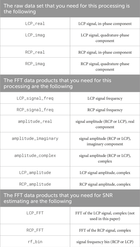
3 The raw data

The following methodology is detailed due to the nature of radio data. In sharing files, errors will occur with the steps discussed below which are common and costly. Thousands to millions of samples per second can be collected for analysis, and processing these files for the uninitiated can be intimidating. Jensen (2007) includes a newly published Zenodo archive of the raw data files in addition to the (Jensen and Russell, 2007) processing codes. Following this text with those materials is the best place to start for accessing this data for the uninitiated. The received data that is being discussed in this article was too much for the code in Jensen (2007) to manage without more powerful processing tools. However, the reader should note that if there is concern about the output from their algorithm, the technique used in Jensen and Russell (2007) can be used to verify plane of polarization measurements.

Radio data will come in a variety of formats, and it is not unusual to have to write new code in order to read the file. Often there is some help with this from the observer or observing facilities, but the most important step is to make sure that you have the proper byte order also known as ‘endian’ for the file. Make sure that whoever recorded the data gives you sufficient details to pull out the first 10–50 points and compare to a separate output that they provide.

When the points are properly decoded from binary to ascii, the next step is to assemble them into the recorded data streams. Old Digital Sampling Processors (DSPs) only collected a single stream of data for each polarization (example, Magellan from Asmar (1996)). Most modern analog to digital (A2D) processors sample both ‘in-phase’ and ‘quadrature-phase’ components to the wave. By mixing with a cosine wave, the ‘in-phase’ correspond to the real component to a complex wave. The sine wave mixing with the signal gives a ‘quadrature-phase’ for the imaginary component. Together they provide the phase of the wave. These are collected off of each polarization, so the resulting data stream consists of right-handed circularly-polarized (RCP) and left-handed circularly-polarized (LCP) real and imaginary wave components. These four data streams are all nearly simultaneously written into the same binary file. For example, the STEREO signal acquired at GBT was processed through a series of steps from receivers to heterodyning mixers to physical cables attached to a private fast digital sampler (Margot and Giorgini, 2009). Each of these steps can effect the phase difference between the signals.

Polarization data can quickly become confusing as to whether you have the proper magnitude and direction. It’s not uncommon to process your whole data set and then realize that the assignment of right-/left-handed in-/quadrature-phase was not what you initially thought it was. This is usually due to human error (miscommunication) at various stages in signal acquisition and post-processing. Consequently, you need to retain enough information to be able to repair the output. Re-running the raw data is often too tedious and time consuming to be feasible. For example, in producing this paper we discovered that the cables connecting the antenna to our analog-to-digital (A2D) sampler had been switched. All spacecraft manufactured to interface with the JPL/Deep Space Network transmit right-handed as the dominant polarization. In 2014, this was in the first channel recorded by the A2D, so we initially assumed this was the case in 2015. The 2015 data from STEREO A was more complicated by the fact it was obtained from the side lobes where the distribution of polarization is more linear. On inspecting MESSENGER data collected in 2015, it became clear that the right-handed polarization was now in the second channel of the A2D. As a result, we added a note of caution to users of the Zenodo archive of this paper’s data.

3.1 Plane of polarization

Sometimes you are provided a code for obtaining the plane of polarization. Other times you must develop your own data processing techniques. In either case you need to construct a test signal of simulated data and make sure that the input plane of polarization is returned. The first step is to subtract off the mean, the DC part of the signal. If left in, the FFT spectrum will be dominated by the curve towards zero, making it difficult to detect the signal. Next the signal needs to be inspected for its phase characteristics. To do this, the FFT is calculated with the complex waves, giving a phase angle; this is $\phi$ in Equation 2:

phase = atan2(amplitude_imaginary, amplitude_real)

= angle(amplitude_complex)

In the case of the STEREO data set, the signal phases written to the file were often both rotating in the same direction (see the Section 6.1). This caused a problem in the calculation of the phase for RCP and LCP:

PP = (angle(LCP_amplitude)+angle(RCP_ amplitude))/2

We were unable to determine why this occurred; however, information on when it occurred is provided in the Section 6.1. Consequently, we examined what would happen when the time series for the LCP was manually flipped to the negative:

PP =

(

-1*sign(LCP_signal_freq)*sign(RCP_signal_freq)

*angle(LCP_amplitude)

)

+ angle(RCP_amplitude))/2

The result was that the correct plane of polarization was returned in our simulated data. Using this same calculation accounting for the sign of the frequency later proved consistent within the actual data. Consequently, one of the polarization signs needs to be reversed; identifying which one takes some thought. For our circumstances, the dominant polarization was the RCP, with the production of the LCP occurring due to cross-polarization leakage. For other data sets, this approach may need to be modified, but that will become clear as the angles are calculated.

The next issue that needs to be addressed is balancing. The amplitudes of the in-phase and quadrature-phase signals should be relatively equal, but this may not be the case due to various circumstances in the dataset that has been collected. Any mixing or amplification of the signal after the in-phase and quadrature-phase separation of the signal can cause an imbalance. To inspect this effect, a test signal (simulated data) was run with these phases given different amplitudes and the plane of polarization that was returned was not the one that was input. Following the balancing step, it came through clearly.

So the next calculation that needs to be performed prior to calculating the FFT is to normalize the imaginary parts of the signal:

RCP_imag = RCP_imag*mean(abs(RCP_real))/mean(abs(RCP_imag))

LCP_imag = LCP_imag*mean(abs(LCP_real))/mean(abs(LCP_imag))

The next calibration step is to compare different methods for calculating the plane of polarization. The ones that we investigate in this paper are the following: (a) plane of polarization angle from direct FFT calculation (Figure 2, top left panel), (b) plane of polarization angle from Stokes parameters (top right panel), (c) plane of polarization angle from Stokes parameters with amplitudes of LCP and RCP at the RCP frequency (eliminates the 90° instability) (middle left panel), and (d) plane of polarization angle from Stokes parameters with amplitudes of LCP and RCP following lowpass Butterworth filtering of the RCP frequency for selecting the specific frequency bin in the unfiltered FFT spectra (middle right panel). The reader is encouraged to review Radio Astronomy by Kraus (Kraus, 1973) to review Stokes parameters.

Figure 2

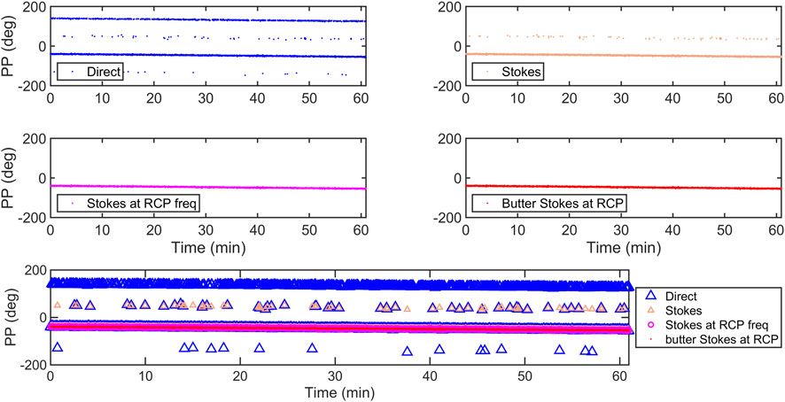
Figure 2. Comparison of different approaches to measuring the plane of polarization. Observation date was 2015 February 7 with STEREO-A. For the remainder of the paper, we will be looking at the PP as calculated with a butter filtered RCP frequency used to select which FFT amplitudes to use for the Stokes calculations (middle right panel).

To be clear, when we state that the complex amplitudes at the RCP frequency are being used, this is what it means:

RCP_amplitude = RCP_FFT(RCP_signal_freq)

LCP_amplitude = LCP_FFT(RCP_signal_freq)

Figure 2 shows a comparison of these different approaches (individual approaches in the top and middle panels, then all-together in the bottom). The PP obtained from Stokes calculations using unfiltered FFT amplitudes at the signal frequency obtained from the butter filtered RCP frequency performed the best. For the remainder of the paper, we will be looking at the PP calculated in this manner. In the current calculation, we focus only on amplitudes from the frequency bin with the strongest signal:

RL = (RCP_amplitude)*conjugate(LCP_amplitude)

I = (abs(RCP_amplitude)^2)+(abs(LCP_amplitude)^2)

Q = 2*real(RL)

U = 2*imag(RL)

V = (abs(LCP_amplitude)^2) - (abs(RCP_amplitude)^2)

PP = 0.5*atan2(U,Q)

As Figure 2 shows, the Stokes parameters do not eliminate the $\pm 180$ degrees ambiguity, rather the solution space is reduced to $\pm 90$ degrees. A $\pm 90$ degree ambiguity is also present, until the amplitudes of the LCP FFT at the RCP frequency are used. The suspected cause for why this works is because the source of the LCP signal is cross-polarization leakage on the transmission system. Concern that the signal in this form is not accurately rotating was settled by observations of STEREO’s rotation when it was set at a 5°/minute rotation rate in March 2015 (shown in this paper below).

3.2 Signal-to-noise ratio

The noise of the system and the signal-to-noise ratio (SNR) of the observation are important measurements to make for calibration, impacting the ${\chi }_j$ component of the plane of polarization in Equation 3. While this technique is ONLY for spacecraft observations, the SNR analysis result shown in Figure 3 can apply more generally.

Figure 3

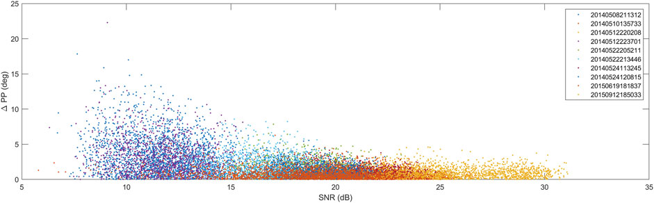
Figure 3. For the various observations in which the rotation was linear, the difference in the plane of polarization from the mean was calculated and plotted against the SNR in that second of data. The dates for the observations are shown in the format 4-year, 2-month, 2-day, 2-h, 2-min, 2-s. In order, they were collected from the following spacecraft: STEREO-B, STEREO-B, STEREO-A, STEREO-B, STEREO-A, STEREO-B, STEREO-A, STEREO-B, MRO, STEREO-A.

There are certain subtle issues that need to be undertaken for calculating the Signal-to-Noise Ratio (SNR). For example, using the amplitude from the FFT of the signal can spread across multiple frequency bins (rf_bin). Calculating the SNR in the frequency domain requires the noise over the same bandwidth be summed. Most of our signals were one frequency bin in size, 1 Hz, which became an issue with selecting the proper noise level. Any random bin can have highly variable noise values. To address this, we collected some statistics on nearby FFT frequency bins, the mean and the standard deviation. Specifically, we selected 50 bins (Hz range), 25 bins on either side of the 11 bins centered on the signal frequency:

background_noise_low = (RCP_FFT(rf_bin-30 to rf_bin-5))

background_noise_high = (RCP_FFT(rf_bin+5 to rf_bin+30))

background_noise =

concatenate(background_noise_low, background_noise_high)

background_mean = mean(background_noise)

background_std = stdev(background_noise)

background_noise_amplitude = background_mean + background_std

SNR =

20*log10(sqrt(RCP_amplitude_real.^2+RCP_amplitude_imag.^2)

/(background_noise_amplitude))

Another detail to notice here is that the SNR is entirely calculated off of the RCP signal. The LCP signal is significantly weaker. This is another issue with understanding SNR. If the RCP were weaker, then the SNR would be worse as shown. If the cross polarization leakage from the RCP to the LCP were weaker, then the SNR would be worse. The data analysis steps above are enabled by the RCP SNR. The strength of the RCP signal enables further processing to isolate the LCP contribution to the signal. Jensen and Russell (2007) show a technique to enable detecting the LCP signal even with a very weak RCP signal; however, it is computationally intensive, an approach that should only be judiciously applied to a data set of this size. Figure 3 shows the variability of the plane of polarization with the RCP SNR. Specifically, $\mathrm{\Delta }PP$ is the calculated plane of polarization offset (absolute value) from a linearly fit slope. Notice that the smaller the SNR, the greater the variability at that point. There are a few details to recognize: (1) The raw data began with a lower SNR, and this plot is the result after processing to increase the SNR; (2) These are fluctuations about a mean slope, so while the fluctuations can become large, the overall slope can be smaller; (3) The fluctuations do not get smaller than two degrees even with an SNR over 30, a potential result of the radio system or the intervening plasma or both.

With a 1 Hz bandwidth comprising the signal, filtering can assist with improving the SNR. Jensen and Russell (2007) use a very narrow filter, just barely wider than the signal itself. In this calibration article, we use a lowpass filter as the original GHz signal was down-converted to 2.5 MHz range and only a thousand or ten-thousand Hertz range within that window was used for our observations. One issue that arises with using a filter is the impact that it can have on the plane of polarization. When passing data through a filter, the ‘filtfilt’ method was found to retain the phase of the original signal. We utilized a Butterworth filter due to its even response across the frequency window. Many other filters are available which we have not tested. The most important issue with using one is that you want it to preserve the plane of polarization, so that needs to be tested before deploying the filter. We found that even the limited use of the Butterworth filter, to detect the precise signal frequency to select the bin for analysis, improved the SNR of the plane of polarization data.

3.3 The parallactic angle

The parallactic angle is an effect that develops when observing the orientation of an object on the sky, a vector, from a rotational coordinate system. This is an effect on the ${\chi }_j$ component of Equation 3. Analyzing this effect becomes more complicated depending on the type of observing platform; steerable antennas modify the observed parallactic angle. The GBT has a report with the calculation for the parallactic angle, which requires the user to calculate Local Sidereal Time (LST) to determine the hour angle (Lutze, 2025-accessed). The reason we bring this level of detail up is that NAIF/SPICE has a function for calculating Local Solar Time, which can be confused with LST because it is also called LST (Navigation and Ancillary Information Facility, 2025a). In order to calculate LST, we used the material shown in a Virginia Technological Institute lecture (Lutze, 2025-accessed). Figure 4 shows two examples for calculating the parallactic angle (PA). The change in the PA does not match the antenna’s output very well in 2014; this may be due to Faraday rotation. The 2015 observations from a similar vicinity in the sky over GBT indicates that the focus rotation mount does induce a PA (GBT Support Staff, 2025). Calibrating the antenna impacts on the observed polarization needs to be investigated separately, which we will produce in a separate paper.

Figure 4

N)." The bottom graph is labeled "PA South-West" with data from 2015. The y-axis ranges from -200 to 200 degrees, and the x-axis ranges from 0 to 40 minutes in the top graph and 0 to 60 minutes in the bottom graph." id="F4" loading="lazy">

Figure 4. The Green Bank Telescope uses a focus rotation mount, which contributes a parallactic angle (PA) rotation to the plane of polarization. The large discontinuity in the top panel is the result of crossing the highest point in the sky whereupon the hour angle would rotate to a completely different sector for the radio source’s descent. The magenta line shows its placement without the 180° rotation; recall that Stokes parameters modify the solution space to $\pm$ 90°. The bottom panel shows the 2015 observation had very little Faraday rotation. The dates for the observations are shown in the format 4-year, 2-month, 2-day, 2-h, 2-min, 2-s. Top panel spacecraft is STEREO-B, and the bottom panel is STEREO-A.

4 Spacecraft operations effects $\mathrm{o}\mathrm{n}{\chi }_0$

4.1 Spacecraft rotation

As a qualitative check that the Stokes parameters were properly calculated, the spacecraft operations provide useful changes for comparison. Between the observations of STEREO collected in 2014 and 2015, a significant change occurred with respect to STEREO-A: “Note that the Ahead observatory is operating on the second side lobe of the HGA [High Gain Antenna] to prevent overheating of the HGA feed assembly which is currently at 108 °C with the HGA angle at 9.4 °, with respect to the spacecraft-Sun line.” STEREO Science Center (2015a) As shown in the top panel of Figure 5 this manifests as a change in the linearity of the received signal: the less circular it is, the more linear it is. With single-frequency bins for our calculations, we have restricted the Stokes parameters to only polarized solutions, so there is no unpolarized component. STEREO-B was lost on 2014 October 1 Center (2014).

Figure 5

Figure 5. Top panel shows the degree of circular polarization. The main lobe is almost entirely circularly polarized (2014, blue points). The second side lobe is more linearly polarized (2015, red points). Second panel: The variability of the plane of polarization is unaffected despite the two observations being collected from different lobes of the transmitting antenna (STEREO-A). The top and second panels show STEREO-A when it is 3-axis stabilitzed. The third and bottom panels show the change in the STEREO-A plane of polarization before (blue) and after (red) being set into a rotation. Third panel shows the degree of circular polarization; a value of zero indicates that it is entirely linearly polarized. The bottom panel shows the plane of polarization for the time period in the third panel. The dates for the observations are shown in the format 4-year, 2-month, 2-day, 2-h, 2-min, 2-s.

By 2015 March 24, STEREO-A was, “…rotating at 5° per minute on the second HGA side lobe … ” STEREO Science Center (2015b). Figure 5 (third and fourth panels) shows April 20 and March 21 observations, illustrating how these spacecraft rotations manifested. The five degrees per minute rotation is clearly evident (360° from 39 to 108 min into the observation); however, there is some form of increased noise in one part of the side lobe. For calibration purposes, this presents both a challenge and a benefit. The regular spin enables observing absolute Faraday rotation, because the orientation of the spacecraft at a particular point of time is known, changes from the known rotation curve on time scales smaller than the full angle rotation itself would be Faraday rotation. STEREO-A was returned to 3-axis stabilization, no longer spinning, on July 8th Stereo Science Center (2015c).

4.2 Frequency fluctuations

Analysis of Frequency Fluctuations (FF) to characterize changes in Total Electron Content (TEC) density is relatively new (Jensen et al., 2016; Jensen et al., 2024); however, they have been utilized for empirical measures such as turbulence, solar wind speeds, and the location of the Alfvén radius (Efimov et al., 2018; Wexler et al., 2019a; Wexler et al., 2020; Wexler et al., 2021b). These fluctuations manifest as a change in phase with time; therefore, multiple phenomena can contribute to FF. In the case of the transmitted plane of polarization ${\chi }_0$ , FF are important to eliminate/identify spacecraft operations from/with abrupt changes in polarization. FF are also used to detect turbulence characteristics. The FF shown in this paper are calculated by subtracting the Doppler frequency shift from the observed frequency shift.

FF have another benefit with respect to FR observing. With more than one frequency, FF can be used to used to isolate the contribution of the magnetic field perpendicular to the line-of-sight as well as the density. With a single frequency, assumptions have to be made for how the frequency should be varying. In this case, we address the expected Doppler motion by using NASA NAIF/SPICE files (Navigation and Ancillary Information Facility, 2025b). Figure 6 shows what frequency changes are expected from Doppler motion and what are observed. This observing period was selected because we initially thought that the signal shifted from beacon mode to uplink-coherent-phase mode, a spacecraft mission command utilized for a variety of purposes. This is because there is a distinct periodic modification of the frequency. For example, a Differenced Ranging Versus Integrated Doppler (DRVID) signal consists of a predetermined variation in frequency timed in order to obtain the Total Electron Content (TEC) from the group velocity (for example, see Bird and Edenhofer (1990)). As discussed below we determined that spacecraft operations could potentially be ruled out, making the source of this phenomenon unknown.

Figure 6

Figure 6. The unknown phenomena that begins as shown at the 98 min mark did not impact the degree of circular polarization (top panel) or the plane of polarization (second panel). However, it did impact the frequency fluctuation (bottom panel). The fluctuation is calculated from the difference between the predicted Doppler shift and the observed frequency shift (third panel), which is shown in the FF (fourth panel). The date of the observation was 2015 July 25 with STEREO-A.

The modification of the radio frequency signal provides substantial data, enabling examination of the observing conditions. On one observing date, Mars Reconnaissance Orbiter (MRO) showed a signal that ceased to transmit or our antenna drifted off the source for unknown reasons (Figure 7). The cause does NOT appear to be Mars or any unusual natural activity. Inspection of its plane of polarization shows no unusual changes as would be expected if it was rotating; whereas the inspection of the frequency fluctuations could be interpreted as the TEC density may have increased substantially in a short period of time until the signal was lost (red circles in 7 after 16 min). If this were the case, then scintillation of the signal should be apparent in the noise (discussed later) and the Stokes I parameter should show some power loss. While these do occur briefly, the lost signal lasts for the remainder of the observation, lasting a full hour, suggesting a spacecraft operation is occurring. The large discrepancy in the ephemeris prediction versus the observation for Doppler indicates that the spacecraft’s transmission frequency was being modified. A similarly configured uplink-coherent-phase is suspected; however, instead of being used for DRVID, the uplink would be using frequency predictions to adjust for Doppler shifting. Notice how the data is much more consistent in frequency than it would be with Doppler shifting. What is also apparent for this observation period in the data set is that the FF technique for measuring density cannot be used without a second frequency. For example, Jensen et al. (2016) used simultaneous frequency, uplink-phase-coherent data to make density measurements.

Figure 7

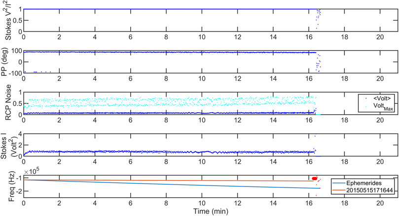
Figure 7. The Mars Reconnaissance Orbiter signal loss. As shown in multiple panels, the MRO signal was lost by our processing algorithm after 16 min of observing (see the middle-right panel of Figure 12 for an example of the signal detected). The top panel shows it is almost entirely circularly polarized; the second panel shows the plane of polarization is relatively fixed with small variability. The third panel shows the background noise in the dominant RCP signal; no unusual density effects are apparent until possibly the last few seconds before the signal loss. The fourth panel shows the Stokes I parameter where the signal is relatively consistent; the fluctuations may be due to data transmission. The bottom panel shows that the predicted Doppler shift was significantly greater than what was measured. The measurements before the signal variations that preceded the loss of signal are shown by the red line. The variations that precede the signal loss are shown by red circles, and the lost signal, random frequencies, are shown by the red dots. The date of the observation was 2015 May 15.

In contrast, the MRO data from 2015 July 4 also shows the signal ceasing to transmit shown in Figure 8. In this case, the cause appears to be Mars, and its surface blocking the signal path between MRO and Earth. A lot of variability occurs in both the noise as well as the Stokes I parameter before it drops. Notice the frequency fluctuations are similar to the STEREO-A data set shown in Figure 6, suggesting a radio operation such as DRVID occurring for the occultation of the Martian ionosphere. We later learned this was not the case (personal email communication with Paul Fiesler). Between our discussion with MRO engineering and our knowledge of the GBT, we discovered that there is no man-made explanation for the periodic FF shown in Figures 6, 8.

Figure 8

Figure 8. Mars Reconnaissance Orbiter occultation by Mars. The top panel shows that the signal was almost entirely circularly polarized. The second panel shows that the plane of polarization was linearly decreasing until the signal passed through the general region of the Martian ionosphere. The third panel shows that the signal was increasing in its noise level, but it briefly dropped midway through the Martian atmosphere. The fourth panel shows that the power in the signal was relatively flat but then became strongly variable in the ionosphere, even increasing. The fifth panel shows that the Doppler prediction and the data were consistent. The bottom panel shows the difference in the fifth panel including a periodic fluctuation in FF in the region of the Martian ionosphere. The date of the observation was 2015 July 4.

The location of the Martian surface relative to the MRO signal to Earth is shown in Figure 9. There were two ephemerides files available for this time frame. After carefully handling the light-time delay, one file showed MRO moving behind Mars from Earth’s view 5 minutes before the observed signal cut off. We asked MRO engineering and learned that the correct ephemeris file was the one which positioned MRO on the limb of Mars at the time of the lost signal, just before it was occulted from Earth’s view (personal email communication with Paul Fiesler). This is an important detail: NAIF documents all the SPICE files utilized by a spacecraft team; however, the team will make updates to these files and it is important to determine which is correct.

Figure 9

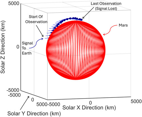
Figure 9. Occultation of MRO by Mars is illustrated. The red sphere is the surface of Mars set to a polar radius, the blue cones are the path of MRO (stepping with time out of the paper toward the viewer), and the blue lines are the lines-of-sight to Earth (into the paper). The associated data is in Figure 8. The solar coordinates shown are IAU Solar Coordinates with the origin set to Mars.

As shown in Figure 7, a portion of the frequency fluctuations has a periodic signature to it. We have confirmed that this occurs when the signal is in a phase-coherent-linked mode with the uplink signal from Earth (reference conversation). As shown in Figure 6, this change is not associated with a change in the plane of polarization for STEREO-A; however, the timing in the second panel of 7 suggests that for the design of the MRO radio system, this may be the case. We do not have other MRO observations to rule out this possibility; however, on communicating with the MRO radio team, we learned that no radio operations were occurring (personal email communication with Paul Fiesler). With respect to STEREO, MESSENGER, and Cassini, it has been ruled out. Based on the lack of any MRO operations, we can conclude that the change in the plane of polarization and the fluctuating frequencies is originating from the Martian ionosphere.

4.3 FFT background noise

4.3.1 Spectral broadening scintillation

One of the issues that we are looking into for supporting calibration is the noise response. The background FFT noise level near the signal can vary significantly under changing plasma conditions. Due to phase scintillation, the signal frequency can spread across a broader frequency range which can be seen in the noise calculations. Phase scintillation can occur due to velocity and/or density changes (see (Bird and Edenhofer, 1990) for more information). It’s an important parameter to detect in the data.

For example, when the maximum and mean of the noise background (background_noise) decreases, while the Stokes I parameter decreases yet remains detectable, this is a strong indicator of signal broadening. This is seen in Figure 10 after 30 min into the time series. At the very beginning for a few seconds similar conditions appear to be present. We have not yet made a direct measure of the signal broadening as the best approach with this data set is still under discussion. An example of what it is in an FFT is shown in the middle left panel of Figure 12.

Figure 10

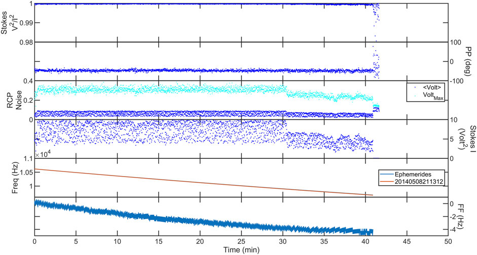
Figure 10. The STEREO-B signal in May 2014. The top panel shows the signal was strongly circularly polarized. The second panel shows that the plane of polarization varied little. The third panel shows that the mean and maximum background noise around the RCP signal decreased after 30 min. The fourth panel shows that the power in the signal decreased at the same time. The fifth panel shows that the Doppler shift varied as predicted. The difference between the two in the sixth panel indicates that the plasma density was decreasing. A scintillation enhancement, signal broadening, occurred during the decrease in maximum noise in addition to the Stokes I parameter. Notice that the FF remain negative, so it is not a density enhancement, making it a velocity change.

Another example of this form of signal broadening is seen in Figure 8 just before the Stokes I parameter begins intensifying (around 25 min). Figure 8 shows when the signal is entirely gone from the observing system, both the mean and max drop to a baseline level. The very end of Figure 10 still has a signal, but we would have to use different processing to acquire it, such as Jensen and Russell (2007). This different signal characteristic is shown in the middle right panel of Figure 12.

4.3.2 No signal VS detecting STEREO B

Even if the precise frequency for the signal has eluded our technique, the fact that the energy is present can be seen from the noise level. An example of the null situation with no source in the beam can be seen with Figure 11, obtained after STEREO-B had been lost. There are a few seconds around 5 min into the observation in which a signal from the spacecraft appeared, but that’s it. Identifying those few seconds in the entire observation is impossible without the noise variation.

Figure 11

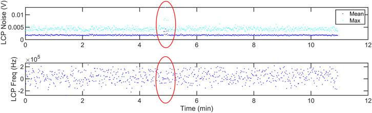
Figure 11. Detection of the STEREO-B signal (red ellipse) after it had been lost in October 2014. The background noise is enhanced and the radio frequency signal is found for a few seconds.

ONE WORD OF CAUTION: While looking at the noise plots is instructive, that’s how we were able to spot the STEREO-B signal, for example, it is for the background_noise around the rf_bin with the maximum value interpreted as the signal (see Section 3.2). If the signal is not detected in the FFT, then the noise is just giving you the noise in any random part of the FFT. While that’s appropriate for noise, the background FFT can have some features to it due to the observing system. Figure 12 from 1 min into the STEREO-B observation, for example, illustrates the falloff in intensity that occurs with higher frequencies; it continues downward for several kHz. In one experiment prior to this one, difficulty with properly downconverting the signal placed it in the band in this higher frequency regime requiring manual detection for configuring the filter.

Figure 12

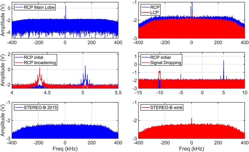
Figure 12. From the data sets shown in Figures 10, 11, the FFT’s are compared. Top left panel shows a RCP FFT near 8 min. Top right panel shows the LCP compared to the RCP. Middle left panel shows signal broadening of the RCP near 36 min compared to the initial RCP in the top left panel. The middle right panel shows the signal as it was being lost shortly after 40 min. The bottom two panels show STEREO-B after it had been lost; most of the observation was like the bottom left panel, but for those few seconds where the noise appeared, so did the signal. This is shown in the bottom right panel.

4.4 Intensity scintillation versus faraday rotation fluctuations

Intensity fluctuations are traditionally studied using variations of frequency transformations. Figure 13 shows the Power Spectral Density (PSD) of each 200 s St-I data in various observation periods shown in this article. A wave is detected in three out of four observations, for data sets shown in Figures 2, 6, 10, with a period of around a few seconds. These are the first such observations of this region of space at this time resolution. They potentially could be related to cyclotron waves with similar periods observed in situ Jian et al. (2014). Note that in the bottom right panel of 13, the subtle fluctuation in Stokes I changes character when the periodic fluctuation in FF occurs after 100 min.

Figure 13

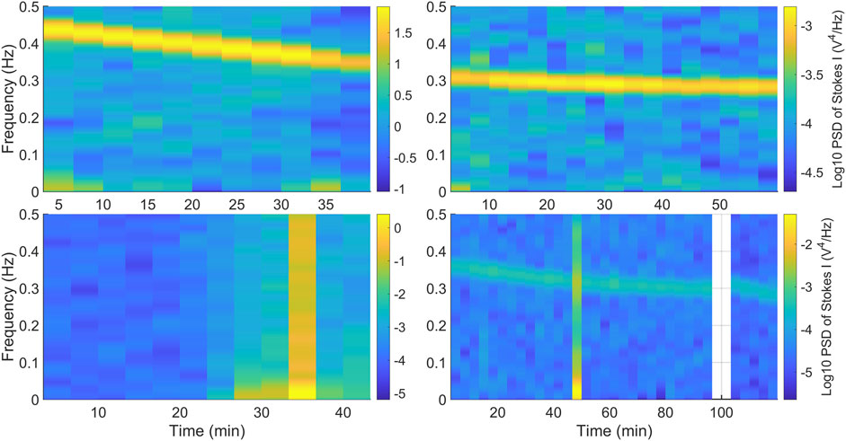
Figure 13. Top left: Power Spectral Density (PSD) of Stokes I measurements with STEREO-B in May 2014 (Figure 10). Top right: PSD of Stokes I data with STEREO-A in February 2015 (Figure 2). Bottom left: PSD of Stokes I data with MRO in July 2015 (Figure 8). Bottom right: PSD of Stokes I with STEREO-A in July 2015 (Figure 6).

The bottom right panel of Figure 13 also shows a brief burst of power around 50 min into the observation. A weaker similar multi-frequency increase in power is near 15 min. Spacecraft operations can cause fluctuations in signal power, but these also cause large discrepancies in frequency. So they are ruled out as a source. Another possible source is radio frequency interference (RFI) in the vicinity of the GBT. The nature of RFI depends on the source and its manifestation in the frequency of interest. While the GBT is in the National Radio Quiet Zone, and works to carefully control RFI near the antenna, bursts of noise occur, and this cannot be ruled out.

For another calibration inspection, the signal intensity variations can then be compared to the Faraday rotation fluctuations (FRF), the change in the plane of polarization presumably from Faraday rotation. What is immediately apparent in comparing Figures 13, 14 is that only the MRO observation shows any correlation. At the time the intensity bursts, the FRF minimizes in variability, suggesting the lines of sight through the Martian magnetosphere varied little, possibly through lensing.

Figure 14

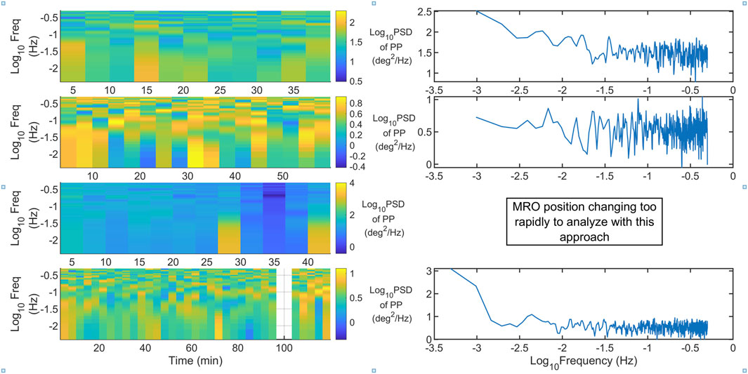
Figure 14. Left: Power Spectral Density (PSD) of the Plane of Polarization with data with observation date (from top to bottom) Figure 10 (STEREO-B May 2014), 2 (STEREO-A February 2015), 8 (MRO July 2015), and 6 (STEREO-A July 2015). Right: the PSD of the entire time series shown on the left, enabling inspection of lower frequency Faraday rotation fluctuations. As shown on the third row, no PSD of the PP could be calculated because the MRO occultation produced such different regimes of behavior. Also note that the bottom right panel utilized the data preceding the data gap shown in the bottom left panel for Stereo-A 2015 July 25.

The right panels in Figure 14 show the Power Spectral Density (PSD) of the entire series of FR for the time period, enabling inspection of the lower frequencies. The top right panel is typical for FRF (e.g., Bird and Edenhofer, 1990). The second right panel is not; the FRF is indistinguishable from white noise for the Stereo-A 2015 February 7 time frame. It potentially may only be detecting the ionosphere; inspection of the location of the line-of-sight within coronal structure will be necessary to understand it.

Keeping in mind the different ordinate axes, the top right and bottom right panels have a similar enhancement in the 0.0032–0.01 Hz range (5.3–1.6 min periods); this is typical behavior of the solar plasmas near the corona (e.g., Efimov et al., 2000).

The lower frequencies as shown by the bottom right panel in Figure 14 of Stereo-A 2015 July 25 are unusual to collect. Usually spacecraft, whether orbiting a planet or simply in its cruise phase, move too fast relative to the Sun to be able to distinguish true lower frequency oscillations from viewing a new aspect of the streaming plasma structure. Because of the unique orbit of STEREO-A, very slowly cruising faster than Earth’s orbit, it’s nearly stationary. For example, during the entire observation period, which was around 120 min, the position of the spacecraft in the sky shifted by $9.54\times 10^3$ km ( $\approx 6.65^{″}$ in the plane of the sky). During the observation period of the MRO occultation lasting 70 min shown in Figure 8, the position of the spacecraft in the sky shifted by $34.46\times 10^3$ km ( $\approx 18.5^{″}$ in the plane of the sky).

Note that for those time periods in which STEREO-A was spinning, distinguishing Faraday Rotation Fluctuations will be very difficult.

5 New techniques pipeline

With respect to intensity fluctuation, the standard approach is to analyze the Stokes I parameter. An experimenter will likely be interested in interpreting differences in amplitude fluctuations between RCP and LCP. For example, we inspected with cross-dipole lab tests how SNR impacted the plane of polarization calculated using amplitudes rather than phase (Gopalswamy et al., 2024). We found that there is a drift in the measured angle with decreasing SNR. In contrast, the Stokes’ derived plane of polarization (which uses phase) was consistent to very low SNR’s.

There is definitely additional information to be developed from analyzing differences between RCP and LCP signals. For example, to our knowledge no one has investigated if the RCP and LCP signals are consistent in characteristics such as their rf_bin or how they vary in their amplitude fluctuations individually. Investigating these details are both more likely to provide better calibration of the observing system as well as new insights into plasma observations. However, as shown in Jensen et al. (2024) for analyzing radio frequency data, it should be undertaken cautiously.

6 Summary

The details for how to begin calibrating spacecraft polarization observations have been provided. The algorithm for processing raw radio frequency voltages needs to be tested with simulated data first to ensure that the input plane of polarization is returned. Then real circumstances such as imbalances between the in-phase and quadrature-phase waves need to be inspected. Any time the data is filtered, its effect on phase and the corresponding plane of polarization needs to be examined.

When complete, the plane of polarization observations combined with other radio measurements enables distinguishing plasma characteristics from transmission radio operations. In some cases these operations can be used for greater insight into plasma properties. If the expected antenna system and plasma effects are not present, then reviewing the previous steps taken in the original data processing needs to be undertaken.

Open questions in our data set include.

• In the case of the STEREO data set, the signal phases written to the file were often both rotating in the same direction; we do not know why this occurred.

• A $\pm 90$ degree ambiguity was occasionally present in the plane of polarization until the amplitudes of the LCP FFT at the RCP frequency rf_bin were used; the suspected cause for why was that the source of the LCP signal is cross-polarization leakage on the transmission system.

• A wave period of a few seconds is detected in multiple observations under discussion for this paper shown in Figure 13; as this data set is the first to be able to resolve such a phenomenon, we’re uncertain as to its source.

Calibration is a continuing process. Calibrating the solar observations we collected in particular is challenging, because the transmitter is changing, the observing takes place infrequently, and the intervening plasma is varying across multiple scales. Spacecraft operations add their own unique benefits/challenges.

Details we bring up in this paper to be addressed in the near future include the following. Using NAIF files, we should be able to estimate to a high accuracy the orientation of the spacecraft at a particular point in time. With this knowledge, understanding how best to incorporate the calibration observations collected of known radio-astronomical sources to model the antenna response will be undertaken. We will compile observations of the periodic fluctuations in FF across multiple missions of Faraday rotation observing experiments. We will investigate if there are DRVID TEC measurements to add to these observations. Similarly, we will investigate what calibration steps can be taken for those observations where the observed frequency is nearly fixed and nowhere close to the expected Doppler frequency, an uplink-coherent-phase locked condition. We will also investigate the Martian ionospheric observations collected and compare them to other MRO instruments observing the region detected of the Martian atmosphere. Finally, we will complete the processing for acquiring a signal broadening scintillation measure and inspect its utility for detecting average plasma velocity when used with frequency fluctuations in the signal intensity due to TEC changes.

6.1 Digitized polarization

The following segment of code illustrates the issues we encountered with polarization observations. The left-handed (LCP) phase should advance in a negative sense, generating a negative frequency. This was rarely the case. As we found with testing, obtaining the correct plane of polarization was the result of accounting for the sign of the LCP being incorrect and adjusting.

data=load(’data20140508211312.010.result.csv’);

tvec=data(:,1);

rangle=angle(data(:,5)+1j*data(:,6));

langle=angle(data(:,8)+1j*data(:,9));

lfreq=data(:,7);

rfreq=data(:,4);

figure,subplot(2,1,1),plot(tvec,sign(rfreq),’linewidth’,2),hold on,

plot(tvec,sign(lfreq),’--’)

ylabel(’Advancing Phase Direction’),

legend(’RCP’,’LCP’,’location’,’southwest’)

subplot(2,1,2),plot(tvec,(-1*sign(lfreq).*sign(rfreq).*.

langle+rangle)/ $2^{*}$ 180/pi,’.’)

xlabel(’Time in file (sec)’)

ylabel(’Plane of Polarization (deg)’)

hold on,plot(tvec,(langle+rangle)/ $2^{*}$ 180/pi,’ ro’),

hold on,plot(tvec,(-langle+rangle)/ $2^{*}$ 180/pi,’ g^’),

set(gcf, ’Position’, [15, 100, 1500, 400])

legend(’Corrected LCP phase’,’Raw LCP phase’,’Negative LCP phase’,.

’location’,’southwest’)

fn=“LCPphaseflip.png”;

figure,exportgraphics(gcf,fn,“Resolution”,300)

As shown in the Figure 15 produced by this code, the plane of polarization was correctly determined when the LCP frequency was negative. Otherwise, the result was noise. When the phase of the LCP was multiplied by a negative, the correct planes of polarization were retrieved for all except the few that were correct initially. Hence, the final plane of polarization was obtained by accounting for whether the LCP was advancing in the correct direction or not.

Figure 15

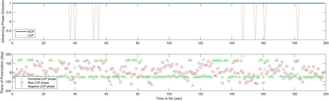
Figure 15. When the LCP frequency is negative from the LCP phase advancing in the negative direction correctly (top plot), the plane of polarization (PP) is correct (where the red circles and blue dots align). Otherwise, the LCP phase angle needs to be reversed by multiplying by a negative to obtain the correct PP (green triangles). For properly processing an issue like this, the direction of the advancing phase needs to be addressed (blue dots).

Data availability statement

The original contributions presented in the study are included in Jensen et al. 2025, further inquiries can be directed to the corresponding author.

Author contributions

EJ: Project administration, Validation, Visualization, Data curation, Methodology, Conceptualization, Formal Analysis, Writing – original draft, Supervision, Funding acquisition, Writing – review and editing, Resources, Software, Investigation. AK: Project administration, Data curation, Writing – review editing, Investigation. DW: Data curation, Investigation, Methodology, Writing – review and editing. AK: Methodology, Data curation, Investigation, Writing – review and editing. JK: Visualization, Methodology, Data curation, Resources, Investigation, Writing – review and editing, Supervision, Formal Analysis. AV: Investigation, Writing – review and editing. AC: Investigation, Writing – review and editing. EH-G: Writing – review and editing, Investigation. AK: Investigation, Writing – review and editing. SF: Writing – review and editing, Investigation, Formal Analysis, Methodology, Validation.

Funding

The author(s) declare that financial support was received for the research and/or publication of this article. Basic research at the U.S. Naval Research Laboratory (NRL) is supported by 6.1 Base funding. EA Jensen is President of ACS Engineering & Safety and supported herself working on this project.

Acknowledgements

We would like to thank Carl Heiles, Karen O’Neil, Toney Minter, and the Green Bank Telescope. We would like to thank Paul Fiesler at JPL; Nat Gopalswamy, Lihua Li, and Manohar Deshpande at NASA/GSFC; Juha Vierinen. We would like to thank the Thomas Jefferson High School for Science and Technology Mentorship program and Andrea Cobb for supporting the U.S. Naval Research Laboratory’s Student Volunteer Program. This work was conducted under proposal code GBT15A-355. The National Radio Astronomy Observatory and Green Bank Observatory are facilities of the U.S. National Science Foundation operated under cooperative agreement by Associated Universities, Inc.

Conflict of interest

Author EJ was employed by the company ACS Engineering & Safety.

The remaining authors declare that the research was conducted in the absence of any commercial or financial relationships that could be construed as a potential conflict of interest.

Generative AI statement

The author(s) declare that no Generative AI was used in the creation of this manuscript.

Any alternative text (alt text) provided alongside figures in this article has been generated by Frontiers with the support of artificial intelligence and reasonable efforts have been made to ensure accuracy, including review by the authors wherever possible. If you identify any issues, please contact us.

Publisher’s note

All claims expressed in this article are solely those of the authors and do not necessarily represent those of their affiliated organizations, or those of the publisher, the editors and the reviewers. Any product that may be evaluated in this article, or claim that may be made by its manufacturer, is not guaranteed or endorsed by the publisher.

References

Asmar, S. W. (1996). Two-wavelength faraday rotation measurement in the solar corona. Master’s thesis. Northridge, United States: California State University.

Google Scholar

Barthel, P. D., Schilizzi, R. T., Miley, G. K., Jagers, W. J., and Strom, R. G. (1985). The large and small scale radio structure of 3C 236. Astronomy Astrophysics 148, 243–253.

Google Scholar

Bauer, S. J., and Daniels, F. B. (1958). Ionospheric parameters deduced from the faraday rotation of lunar radio reflections. J. Geophys. Res. 63, 439–442. doi:10.1029/JZ063i002p00439

CrossRef Full Text | Google Scholar

Bell, M. B., Covington, A. E., and Kennedy, W. A. G. (1973). Polarization interferometer for 2800 MHz solar noise studies with a 0.5’ fan beam. Sol. Phys. 28, 123–136. doi:10.1007/BF00152917

CrossRef Full Text | Google Scholar

Bird, M. K., and Edenhofer, P. (1990). “Remote sensing observations of the solar Corona,” in Physics of the inner heliosphere I. Editors R. Schwenn, and E. Marsch (Berlin Heidelberg: Springer-Verlag), 13–97.

CrossRef Full Text | Google Scholar

Bird, M. K., Volland, H., Howard, R. A., Koomen, M. J., Michels, D. J., Sheeley, N. R., et al. (1985). White light and radio sounding observations of coronal transients. Sol. Phys. 98, 341–368. doi:10.1007/BF00152465

CrossRef Full Text | Google Scholar

Efimov, A. I., Samoznaev, L. N., Andreev, V. E., Chashei, I. V., and Bird, M. K. (2000). Quasi-Harmonic faraday-rotation fluctuations of radio waves when sounding the outer solar Corona. Astron. Lett. 26, 544–552. doi:10.1134/1.1306991

CrossRef Full Text | Google Scholar

Efimov, A. I., Lukanina, L. A., Chashei, I. V., Bird, M. K., Pätzold, M., and Wexler, D. (2018). Velocity of the inner solar wind from coronal sounding experiments with spacecraft. Cosmic Res. 56, 405–410. doi:10.1134/S0010952518060023

CrossRef Full Text | Google Scholar

Efimov, A. I., Lukanina, L. A., Chashei, I. V., Bird, M. K., and Pätzold, M. (2019). Solar wind magnetic field turbulence over the solar activity cycle inferred from coronal sounding experiments with helios linear-polarized signals. Astron. Rep. 63, 174–181. doi:10.1134/S106377291903003X

CrossRef Full Text | Google Scholar

GBT Support Staff (2025). Observer’s guide for the green bank telescope

Google Scholar

Gopalswamy, N., Fung, S. F., Hughes, P. M., Nolfo, G. A. D., Paschalidis, N., and Summerlin, E. J. (2024). Breadboarding FETCH, theSTEREO MOC Status Report Time Period Faraday Effect Tracker for Coronal and Heliospheric Structures (FETCH). Greenbelt, MD: Center Independent Research & Development: GSFC IRAD. Technical Report

Google Scholar

Hollweg, J. V., Bird, M. K., Volland, H., Edenhofer, P., Stelzried, C. T., and Seidel, B. L. (1982). Possible evidence for coronal Alfvén waves. J. Geophys. Res. 87, 1–8. doi:10.1029/JA087iA01p00001

CrossRef Full Text | Google Scholar

Jensen, E. A. (2007). High frequency Faraday rotation observations of the solar corona. Los Angeles, United States: Ph.D. thesis, University of California.

Google Scholar

Jensen, E. A., and Russell, C. T. (2007). “Measuring the plane of polarization in a strongly circular signal,” in Solar physics and space weather instrumentation II. 6689 of society of photo-optical instrumentation engineers (SPIE) conference series . Editors S. Fineschi, and R. A. Viereck doi:10.1117/12.734860

CrossRef Full Text | Google Scholar

Jensen, E. A., Frazin, R., Heiles, C., Lamy, P., Llebaria, A., Anderson, J. D., et al. (2016). The comparison of total electron content between radio and Thompson scattering. Sol. Phys. 291, 465–485. doi:10.1007/s11207-015-0834-5

CrossRef Full Text | Google Scholar

Jensen, E. A., Heiles, C., Wexler, D., Kepley, A. A., Kuiper, T., Bisi, M. M., et al. (2018). Plasma interactions with the space environment in the acceleration region: indications of CME-trailing reconnection regions. Astrophysical J. 861, 118. doi:10.3847/1538-4357/aac5dd

CrossRef Full Text | Google Scholar

Jensen, E. A., Rahmani, Y., and Simpson, J. J. (2024). The hunt for perpendicular magnetic field measurements in plasma. Astrophysical J. 963, 25. doi:10.3847/1538-4357/ad2347

CrossRef Full Text | Google Scholar

Jensen, E., Kepley, A., Wexler, D., Kobelski, A., Kooi, J., Valliani, A., et al. (2025). Spacecraft radio signal polarization calibration. doi:10.5281/zenodo.15602915

CrossRef Full Text | Google Scholar

Jian, L. K., Wei, H. Y., Russell, C. T., Luhmann, J. G., Klecker, B., Omidi, N., et al. (2014). Electromagnetic waves near the Proton cyclotron frequency: STEREO observations. Astrophysical J. 786, 123. doi:10.1088/0004-637X/786/2/123

CrossRef Full Text | Google Scholar

Kaiser, M. L., Kucera, T. A., Davila, J. M., St. Cyr, O. C., Guhathakurta, M., and Christian, E. (2008). The STEREO mission: an introduction, Space Sci. Rev. STEREO Mission An Introd. 136, 5–16. doi:10.1007/s11214-007-9277-0

CrossRef Full Text | Google Scholar

Kobelski, A., Jensen, E., Wexler, D., Heiles, C., Kepley, A., Kuiper, T., et al. (2016). “Measuring the solar magnetic field with STEREO A radio transmissions: faraday rotation observations using the 100m Green bank telescope,” in Coimbra solar physics meeting: ground-based solar observations in the space instrumentation era. 504 of astronomical society of the Pacific conference series Editors I. Dorotovic, C. E. Fischer, and M. Temmer, 99, 99K.

Google Scholar

Kooi, J. E., Wexler, D. B., Jensen, E. A., Kenny, M. N., Nieves-Chinchilla, T., Wilson, L. B., et al. (2022). Modern faraday rotation studies to probe the solar wind. Front. Astronomy Space Sci. 9, 841866. doi:10.3389/fspas.2022.841866

CrossRef Full Text | Google Scholar

Kraus, J. D. (1973). Radio astronomy. Delaware, OH, United States: Cygnus-Quasar Books.

Google Scholar

Lam, M. T., Cordes, J. M., Chatterjee, S., Jones, M. L., McLaughlin, M. A., and Armstrong, J. W. (2016). Systematic and stochastic variations in pulsar dispersion measures. Astrophysical J. 821, 66. doi:10.3847/0004-637X/821/1/66

CrossRef Full Text | Google Scholar

Le Chat, G., Kasper, J. C., Cohen, O., and Spangler, S. R. (2014). Diagnostics of the solar Corona from comparison between faraday rotation measurements and magnetohydrodynamic simulations. Astrophysical J. 789, 163. doi:10.1088/0004-637X/789/2/163

CrossRef Full Text | Google Scholar

Lutze, F. H. (2025). Time Considerations- local sidereal time. Tech. Rep., Va. Tech Dep. Aerosp. Ocean Eng.

Google Scholar

Lyne, A. G., Smith, F. G., and Graham, D. A. (1971). Characteristics of the radio pulses from the pulsars. Mon. Notices R. Astronomical Soc. 153, 337–382. doi:10.1093/mnras/153.3.337

CrossRef Full Text | Google Scholar

Margot, J.-L., and Giorgini, J. D. (2009). “Probing general relativity with radar astrometry in the inner solar system”, 41. IAU Symp American Astronomical Society.

Google Scholar

Navigation and Ancillary Information Facility (2025a). Navigation and ancillary information facility ET2LST . Pasadena, CA: ET to Local Solar Time.

Google Scholar

Navigation and Ancillary Information Facility (2025b). SPICE (spacecraft, planet, instrument, C-matrix, events): An Observation Geometry System for Space Sscience Missions Pasadena, CA: Jet Propulsion Laboratory

Google Scholar

Parker, E. N. (1966). The dynamical state of the interstellar gas and field. Astrophysical J. 145, 811. doi:10.1086/148828

CrossRef Full Text | Google Scholar

Ruiz-Granados, B., Battaner, E., and Florido, E. (2016). Searching for faraday rotation in cosmic microwave background polarization. Mon. Notices R. Astronomical Soc. 460, 3089–3099. doi:10.1093/mnras/stw1157

CrossRef Full Text | Google Scholar

STEREO Science Center, S. S. (2014). STEREO MOC status report time period: 2014:272 – 2014:278. Greenbelt, MD: NASA, Technical Report

Google Scholar

STEREO Science Center (2015a). “STEREO MOC status report time period: 2015:026 – 2015:032,”. Greenbelt, MD: NASA, Technical Report.

Google Scholar

STEREO Science Center (2015b). “STEREO MOC status report time period: 2015:082 – 2015:088,” Greenbelt, MD: NASA, Technical Report.

Google Scholar

STEREO Science Center (2015c). “STEREO MOC status report time period: 2015:187 – 2015:193,”. Greenbelt, MD: NASA, Technical Report.

Google Scholar

Wexler, D. B., Hollweg, J. V., Efimov, A. I., Lukanina, L. A., Coster, A. J., Vierinen, J., et al. (2019a). Spacecraft radio frequency fluctuations in the solar Corona: a MESSENGER-HELIOS composite study. Astrophysical J. 871, 202. doi:10.3847/1538-4357/aaf6a8

CrossRef Full Text | Google Scholar

Wexler, D. B., Hollweg, J. V., Efimov, A. I., Song, P., Jensen, E. A., Lionello, R., et al. (2019b). Radio occultation observations of the solar Corona over 1.60-1.86 R: faraday rotation and frequency shift analysis. J. Geophys. Res. Space Phys. 124, 7761–7777. doi:10.1029/2019JA026937

CrossRef Full Text | Google Scholar

Wexler, D., Imamura, T., Efimov, A., Song, P., Lukanina, L., Ando, H., et al. (2020). Coronal electron density fluctuations inferred from akatsuki spacecraft radio observations. Sol. Phys. 295, 111. doi:10.1007/s11207-020-01677-1

CrossRef Full Text | Google Scholar

Wexler, D. B., Jensen, E. A., and Heiles, C. (2021a). Middle Corona magnetic field strength determined by spacecraft radio faraday rotation. Res. Notes Am. Astronomical Soc. 5, 165. doi:10.3847/2515-5172/ac1521

CrossRef Full Text | Google Scholar

Wexler, D. B., Stevens, M. L., Case, A. W., and Song, P. (2021b). Alfvén speed transition zone in the solar Corona. Astrophysical J. 919, L33. doi:10.3847/2041-8213/ac25fa

CrossRef Full Text | Google Scholar