The connection of the Ions and electrons in the Earth’s central plasma sheet to the solar wind

The simple problems of the solar wind number density driving the plasma sheet number density and the solar wind speed driving the plasma sheet temperature are examined. To ensure that the central plasma sheet is studied, 1017 current sheet crossings in the plasma sheet are collected from 10.8 R_E to 76.9 R_E downtail, and 3-s resolution ion and electron measurements from THEMIS-B and THEMIS-C are compared with time-lagged solar wind number densities and speeds. The central plasma sheet measurements are taken from the solar minimum years of 2007–2009. Three correlation methods are used: (1) Pearson (univariate) linear correlations; (2) multivariate linear correlations; (3) canonical correlation analysis. For both ions and electrons, knowing the solar wind speed adds insignificant information to the solar wind density versus plasma sheet density correlations. Likewise, for both ions and electrons, knowing the solar wind density adds insignificant information to the solar wind speed versus plasma sheet temperature correlations. The standard two problems (1) the density of the solar wind driving the density of the plasma sheet and (2) the velocity of the solar wind driving the temperature of the plasma sheet, appear to be completely unrelated, even though the solar wind density and the solar wind velocity have a strong anticorrelation. Future work is outlined.

1 Introduction

Understanding how the solar wind controls the plasma content and energy in the Earth’s central plasma sheet (Bame et al., 1966, 1967; Hones et al., 1971) remains a fundamental challenge in space-physics research. Despite decades of observations, the precise way in which upstream parameters such as solar wind density, velocity, and interplanetary magnetic field (IMF) orientation regulate the plasma sheet’s properties is still under active investigation. Moreover, the timing and spatial patterns of this coupling remain only partially understood.

Numerous studies have demonstrated that solar wind conditions (e.g., density and velocity) are strongly coupled with plasma properties in Earth’s central plasma sheet. Observationally, slow and dense solar winds under low geomagnetic activity tend to produce a colder and denser plasma sheet (Thomsen et al., 2003; Lavraud et al., 2006a; Lavraud et al., 2006b; Borovsky and Steinberg, 2006), whereas fast and tenuous solar winds lead to a hotter and more tenuous plasma sheet. This pattern “slow/dense solar wind yielding cold/dense plasma sheet” versus “fast/tenuous solar wind yielding hot/tenuous plasma sheet” was first reported in Wind/Geotail studies (Terasawa et al., 1997) and later confirmed by additional statistical analyses (Borovsky et al., 1998a; Yan et al., 2005).

In particular, Borovsky et al. (1998a) showed that the ion density in the central plasma sheet positively correlates with the solar wind density, while the temperature in the central plasma sheet positively correlates with the solar wind velocity. Theoretically, this coupling reflects how solar wind plasma enters the magnetosphere. During prolonged northward IMF, cold and dense magnetosheath plasma can be transported to the magnetotail via Kelvin–Helmholtz instabilities or lobe–lobe reconnection, forming the cold dense plasma sheet (CDPS). In contrast, during southward IMF and active geomagnetic conditions, tail reconnection injects lower-density, higher-energy plasma, yielding a hot and tenuous central plasma sheet. This dichotomy has been corroborated by observational profiles of the plasma sheet distinguishing northward versus southward IMF conditions (Wing and Newell, 2002).

Solar wind plasma can reach the magnetotail plasma sheet within only a few hours. Borovsky et al. (1998a) and Denton and Borovsky (2009) performed statistical timing analyses and found that solar wind particles take on the order of ∼2 h to reach the mid-tail plasma sheet (downtail at ∼15–25 $R_E$) and ∼4 h to reach the near-Earth plasma sheet in the nightside dipolar region. In case studies wherein sudden number density increases in the solar wind were timed as they entered the magnetotail and were advected Earthward into the nightside dipolar region and then around into the dayside magnetosphere (c.f. Figures 5 and 6 of Denton and Borovsky (2009)), the event timing agreed with time lags in statistical studies. Recent cross-correlation studies confirm similar response lags on the order of a few hours. For example, a coordinated MMS–ARTEMIS observation found that solar wind density fluctuations take about 3.7–5.9 h to propagate into the plasma sheet to make the cold dense plasma sheet (Yu et al., 2020), consistent with earlier single-satellite inferences. These time lags indicate a relatively prompt coupling, on the scale of a substorm cycle, between upstream solar wind changes and the central plasma sheet’s properties.

Multiple studies report a positive correlation between solar wind density (or dynamic pressure) and plasma sheet density. Simply put, when the shocked solar wind magnetosheath is denser, more plasma leaks into the magnetotail via reconnection or via low-latitude-boundary-layer processes. Borovsky et al. (1998a), using 244 encounters of ISEE-2 with the neutral sheet in the magnetotail at downtail distances from 17.5 to 22.5 R_E, showed that plasma sheet pressure (and by implication, particle content) is strongly correlated with solar wind ram pressure, with correlation coefficients being approximately 0.84. More recently, Yan et al. (2005) analyzed Double Star (TC-1) observations at ∼9–13.4 $R_E$ and confirmed that increases in upstream solar wind density (or solar wind dynamic pressure) lead to increased plasma sheet density in the near-Earth tail (Yan et al., 2005). In fact, those Double Star results demonstrated that the solar wind dynamic pressure controls the ion thermal pressure in the central plasma sheet as well. Together, these findings support a picture in which a denser or more forceful solar wind feeds the plasma sheet with additional plasma, raising its density and particle pressure.

The solar wind speed also influences the plasma sheet plasma energy. Under typical conditions (e.g., southward IMF), faster solar wind streams carry more energy into the magnetosphere and tend to correlate with higher ion temperatures in the plasma sheet. For instance, Borovsky et al. (1998a) found a positive (though moderate) correlation between solar wind flow speed and plasma sheet ion temperature, consistent with faster solar wind flows creating hotter magnetosheath plasma bathing the magnetosphere, thereby injecting hotter plasma into the magnetosphere. However, the relationship can reverse under prolonged northward IMF conditions. During northward IMF, the plasma sheet often becomes “cold and dense,” filled by magnetosheath-origin plasma without substantial heating upon entry (Lavraud et al., 2006a; Lavraud et al., 2006b; Forsyth et al., 2014). This process is supported by observations of plasma transport across the flanks of the magnetopause via Kelvin–Helmholtz instabilities and lobe reconnection under northward IMF, as reviewed by Walsh et al. (2014). Under northward IMF (and hence quiet geomagnetic activity), the entry may be predominantly via the low-latitude boundary layer and via magnetic reconnection beyond the cusps, which might not yield the higher plasma energization as does dayside reconnection. This was shown by the statistical maps of Wing and Newell (2002): during northward IMF periods, the plasma sheet’s temperature drops even as solar wind conditions intensify, whereas during southward IMF, the plasma sheet is hotter and more tenuous. Thus, solar wind velocity has a dual effect, generally boosting plasma sheet temperature, but only when the upstream magnetic configuration allows efficient energization (southward IMF); under opposite conditions (northward IMF), studies indicate that fast solar wind mainly increases plasma sheet density at the expense of temperature.

Beyond simple one-to-one correlations, empirical models have quantified how multiple solar wind factors jointly regulate plasma sheet properties. Tsyganenko and Mukai (2003) developed an analytic model of the central plasma sheet (≈10–50 $\left.R_E\right)$ based on Geotail spacecraft data. Their model equations describe plasma sheet ion density, temperature, and pressure as functions of location and upstream conditions. The results indicated that solar wind drivers, such as dynamic pressure and IMF orientation, significantly affect plasma sheet pressure and density distributions. In the near-Earth plasma sheet (r < ∼15 $\left.R_E\right)$, solar wind ram pressure was found to be a primary influence on plasma sheet total pressure, while IMF B_z (southward component) influenced plasma sheet thickness and density (Walsh et al., 2014).

Dubyagin et al. (2016) created empirical relations for plasma sheet electron density and temperature (at 6–11 $\left.R_E\right)$ during geomagnetic storms using time-averaged solar wind inputs. Their statistical model achieved a very high correlation (∼0.8 linear correlation) between predicted and observed plasma sheet parameters using THEMIS probes. Notably, the plasma sheet density was best reproduced using a ∼4-h average of upstream solar wind proton density, yielding a correlation of r_corr ≈ 0.82 (Dubyagin et al., 2016). Meanwhile, the plasma sheet electron temperature was predicted most accurately by the solar wind bulk velocity (averaged over 4 h) together with IMF factors, achieving a correlation of r_corr ≈ 0.75. These high correlations underscore that incorporating the solar wind’s recent history (several hours of averaging) greatly improves the ability to model plasma sheet conditions. Overall, both older and more recent empirical studies concur that solar wind inputs drive the first-order variations in plasma sheet plasma density and energy content.

Despite these advances, many open questions remain. To what extent can canonical correlation analysis (CCA) improve our understanding of the solar wind to central plasma sheet coupling by incorporating combinations of multiple input and multiple output variables simultaneously? What insights can these techniques provide into the fundamental physical processes responsible for plasma entry and energy transfer from the solar wind into the magnetosphere?

The central plasma sheet acts as the primary plasma and energy reservoir within the magnetosphere. It feeds the ring current, influences radiation belt dynamics, and modulates auroral activity (Kronberg et al., 2014; Borovsky and Valdivia, 2018). Understanding how the plasma sheet responds to solar wind drivers is therefore critical for modeling energy input into the inner magnetosphere and improving space weather forecasting. Better empirical understanding of solar wind to central plasma sheet coupling supports both fundamental geophysics and practical applications, including satellite operation safety and geomagnetic storm prediction.

In the present study, 1017 current sheet crossings are identified in the Earth’s magnetotail at downtail distances of 10.8 R_E to 76.9 R_E. Ion and electron data with 3-s time resolution were used to determine the ion and electron temperatures and number densities for the current sheet crossings to determine values of temperatures and densities in the central plasma sheet at various downtail distances (and under various levels of geomagnetic activity). Correlations of the central plasma sheet properties with the time-lagged solar wind speed and number density are performed (1) with standard Pearson linear correlations; (2) with multivariate linear correlations; (3) with canonical correlation analysis.

This manuscript is organized as follows. In Section 2, both the methodology for selecting the 1017 current sheet crossing events and the data sets used to measure the plasma sheet and solar wind conditions are described. In Section 3, overviews of the number densities and temperatures of the central plasma sheet as functions of downtail distance and level of geomagnetic activity are investigated. In Section 4, correlations between the central plasma sheet and the time-lagged solar wind are performed using various correlation methodologies. Section 5 contains conclusions, discussions, and suggestions for future studies.

2 Data methodology: current sheet crossings and the data analyzed

Using 3-s resolution MAG data (Auster et al., 2008) from THEMIS-B and THEMIS-C, 1017 current sheet crossings (or current sheet encounters) in the magnetotail plasma sheet were identified in 2007–2010 (a solar minimum). Focusing on current sheet crossings is desirable to ensure that the data extracted is from the central plasma sheet, rather than the outer plasma sheet, and to yield the furthest downtail distance of the plasma sheet flux tube. The collected events were restricted to |Y_gse| < 6 R_E and were found from X = −10.9 R_E to X = −76.8 R_E. The positions of the 1017 current sheet crossings are sketched in Figure 1 along with a Fairfield–Greenstadt model of the bow shock position (Fairfield, 1971; Greenstadt et al., 1990) in blue and a Lin et al. (2010) model of the magnetopause location in green. The black points in Figure 1 are the 1017 current sheet crossings, the red points indicate crossings that have THEMIS electron data, the blue points are crossings that have THEMIS ion data, and the purple points are crossings that have both electron and ion data. The crossing events all occurred in the hot plasma of the magnetosphere (T_i > 500 eV) with the encounter or crossing identified as a reversal in the direction of B_x, often with a diamagnetic reduction of the magnitude of B. For each current sheet crossing (event), localized electron data (number density and temperature) were obtained from the 3-s reduced THEMIS ESA data (McFadden et al., 2008) stored on CDAWeb (https://cdaweb.gsfc.nasa.gov), and the ion data (number density and temperature) were obtained from the 3-s THEMIS GMOM data set stored on CDAWeb that utilized the ESA measurements and the higher-energy SST measurements. Solar wind values (number density and speed) at Earth and the Kp index were obtained from the 1-hr-averaged OMNI data set (https://omniweb.gsfc.nasa.gov). The Hp60 geomagnetic index was obtained from ftp://ftp.gfz-potsdam.de/pub/home/obs/Hpo.

Figure 1

Figure 1. A sketch of the position of the bow shock (blue), the position of the magnetopause (green), and the locations of the 1017 THEMIS current sheet crossings in the X-Y plane.

For the neutral sheet crossings, Figure 2A plots the measured ion number density n_i as a function of the measured electron number density n_e, and Figure 2B plots the measured ion temperature T_i as a function of the measured electron temperature T_e. Linear-regression fits are shown as the blue lines. The Pearson linear correlations are r_corr = 0.983 for the number densities and r_corr = 0.837 for the temperatures.

Figure 2

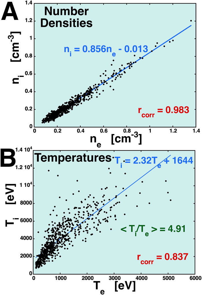
Figure 2. For the current sheet crossings in the central plasma sheet, the measured ion number density is plotted as a function of measured electron density (panel (A)), and the measured ion temperature is plotted as a function of the measured electron temperature (panel (B)).

In the 3-s resolution THEMIS magnetic field data, current sheet crossings can be singular and very rapid (seconds), or the spacecraft can linger in the vicinity of the current sheet region and make multiple crossings. This difference could be due to the presence or absence of magnetotail flapping owing to variations in the solar wind velocity vector. In the collection of 1017 crossings, the shortest time between crossings is 45 s, and the median time between crossings is 20.4 min. No distinction was made between the two types of crossings. Of the 1017 identified events, 891 had ESA electron data temporally close to the crossing times, and 748 had GMOM ion data temporally close to the crossing times.

3 Overview of the ion and electron temperatures and densities in the central plasma sheet

In Table 1, Pearson linear correlation coefficients r_corr between the central plasma sheet electron and ion number densities n_e and n_i and the solar wind number density n_sw and the coefficients between the solar wind velocity v_sw and the central plasma sheet electron and ion temperatures T_e and T_i are collected, with some restrictions in the different rows of the table on the level of geomagnetic activity as measured by Hp60 and on the downtail distance X (in R_E). The numbers in parentheses after each correlation coefficient in Table 1 are the optimal time lag in hours between the solar wind data at Earth and the central plasma sheet data, “optimal” meaning giving the largest-magnitude correlation coefficient.

Table 1

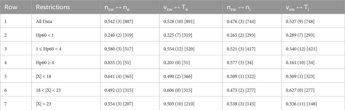
Table 1. The Pearson linear correlations are collected, followed by the optimal time lag in hours in parentheses, followed by the number of data points used in the correlation in brackets.

Row 1 of Table 1 displays the Pearson linear correlation coefficients r_corr for all of the available current sheet crossing data. Scatter plots of Row 1 data appear in the four panels of Figure 3, with panels A and B of Figure 3 showing central plasma sheet electrons and panels C and D showing central plasma sheet ions (protons). If N is the number of data points in the correlation, then correlation at the 95% confidence level occurs for a correlation coefficient with a magnitude larger than 2/N^1/2 (Beyer, 1966; Bendat and Piersol, 2010). With 891 (electrons) and 748 points (ions) in Row 1, the values of the correlation coefficients are many times larger than the 2/N^1/2 values of 0.067 and 0.073.

Figure 3

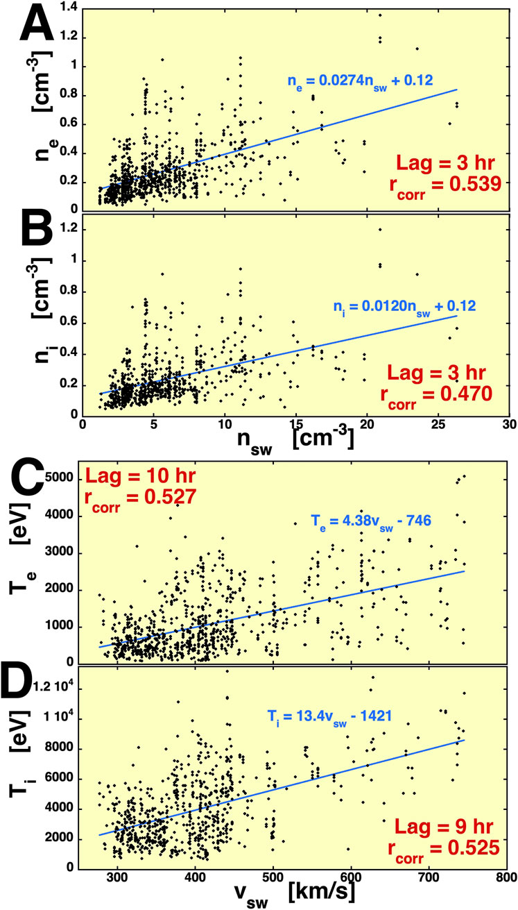
Figure 3. Scatter plots of the electron and ion central plasma sheet number densities and temperatures are plotted as functions of the solar wind number density and speed at Earth. each plot (Panels A-D) indicates the time lag used between the solar wind data and the plasma sheet data.

In Rows 2, 3, and 4 of Table 1, the data are restricted to times of very low geomagnetic activity (Row 2), to times of medium geomagnetic activity (Row 3), and to times of high geomagnetic activity (Row 4). At very low geomagnetic activity, the correlations between the solar wind density and speed and the plasma sheet densities and temperatures are very weak. At medium and high geomagnetic activity (Rows 3 and 4), the correlations between the solar wind and the plasma sheet are much more robust. However, the confidence level of the 0.161 correlation coefficient is very low for the v_sw to T_i correlation in Row 4 for high activity, which has only 34 points to create the correlation, and 2/N^1/2 for N = 34 is 0.340. It is also known that at high levels of geomagnetic activity, the ionosphere becomes an important source of plasma sheet plasma (Young et al., 1982; Lennartsson and Shelley, 1986). Looking at the correlations of solar wind number density and plasma sheet number density with information about the plasma sheet composition would be desirable but is beyond the capabilities of the present study. Note that the correlation study of Borovsky et al. (1998a) was conducted during a solar maximum, where the mean value of Kp was 3.0 for the central plasma sheet events studied, and a high correlation between n_sw and n_p of the plasma sheet was still found, where the electrostatic analyzer measurements of n_p could be contaminated somewhat by O⁺.

In Rows 5, 6, and 7 of Table 1, the correlations are performed for three isolated distance regions of the magnetotail: near the Earth in Row 5, in the middle tail in Row 6, and in the further tail in Row 7. In the table, those electron-density correlation coefficients range from 0.492 to 0.641, the electron-temperature coefficients range from 0.490 to 0.606, the ion-density correlation coefficients range from 0.475 to 0.538, and the ion-temperature coefficients range from 0.336 to 0.627. The middle range 18 < |X| < 23 was chosen to be similar to the range of distances for the “magnetotail neutral sheet” correlations of n_i and T_i that were performed by Borovsky et al. (1998a) for a set of neutral sheet crossings in 1979 by the ISEE-2 spacecraft with the solar wind measured by the ISEE-3 spacecraft. The correlation coefficient was higher for the ISEE n_i measurements (0.74 for ISEE and 0.475 for THEMIS), and the correlation coefficient was lower for the ISEE T_i measurements (0.51 for ISEE and 0.627 for THEMIS. The mean Kp of the ISEE events during solar maximum was 3.0, and the mean Kp of the THEMIS events during the solar minimum was 1.3. Many things in the magnetosphere change with the solar cycle: for example, the level of geomagnetic activity (Echera et al., 2004), the rate of occurrence of substorms (Borovsky and Yakymenko, 2017), the ion composition of the plasma sheet (Young et al., 1982; Lennartsson and Shelley, 1986), magnetotail current systems (Wing et al., 2014), and the types of geomagnetic storms that occur (Borovsky and Denton, 2006). As noted in Rows 2, 3, and 4 of Table 1, the correlations for high activity are large for n_e and n_i and low for T_e and T_i.

4 Interpreting linear correlations, multivariate linear correlations, and canonical correlation analysis

The robust (several times 2/N^1/2 in magnitude where N is the number of data points) positive correlations between (1) the number density of the solar wind and the number density of the central plasma sheet and (2) the velocity of the solar wind and the ion and electron temperatures of the central plasma sheet seem like straightforward evidence that the shocked solar wind (magnetosheath) feeds plasma density into the central plasma sheet and that the temperature of the fed-in plasma is related to the conversion by the bow shock of the cold upstream solar wind into a hot magnetosheath temperature (Phan et al., 1994; Baumjohann, 1993). These simple Pearson linear correlations (PLC) are shown in Rows 1–4 of Table 2. For the solar wind number density, n_sw+3 is taken, which is the solar wind value at Earth 3 h before each current sheet crossing, and v_sw+4 is taken for the solar wind velocity, which is the value at Earth 4 h before each current sheet crossing. This yields time lags from the solar wind at Earth to the reactions in the Earth’s magnetotail, with the time lag being slightly longer for v_sw than for n_sw. The plasma sheet number density coming from the solar wind number density was a strong conclusion of Borovsky et al. (1998a) and of Denton and Borovsky (2009), where the correlation evidence was supported by multiple events wherein observations of sudden increases in the solar wind density at Earth were followed in time as sudden plasma sheet density increase in the nightside magnetotail, then as sudden increases in the nightside dipolar region, and then as increases in the dayside magnetosphere. The Borovsky et al. (1998a) study strongly suggested that the proton temperature of the plasma sheet was related to the shocking of the cold solar wind plasma that would be captured, with the temperature of the magnetosheath plasma behind the bow shock being related to the speed of the solar wind (Kennel, 1988). The temperature ratio T_i/T_e of the plasma sheet being similar to the temperature ratio of the shocked magnetosheath as the solar wind Mach number varies (Lavraud et al., 2009) also supports this picture of conversion of the solar wind speed into temperature across the bow shock. Similarly, Figure 1D of Wang et al. (2012) also supports this point.

Table 2

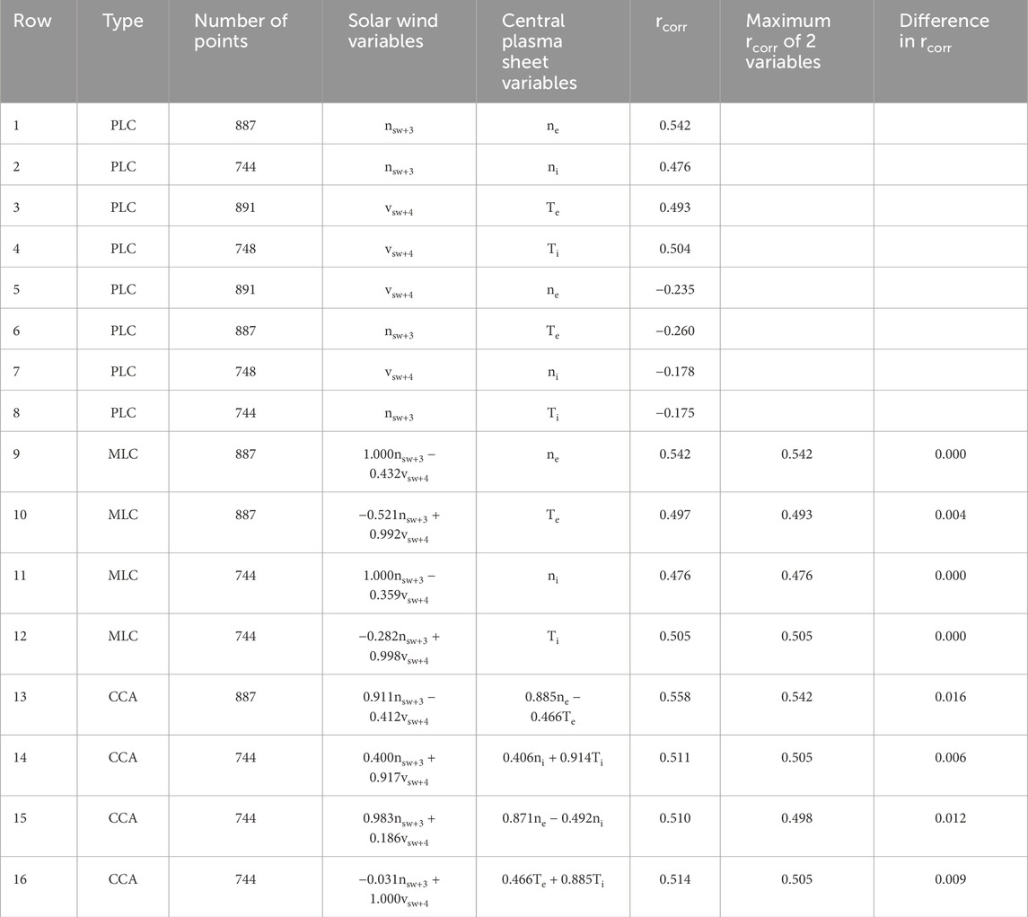
Table 2. The correlation coefficients r_corr for PLC, MLC, and CCA analysis of the central plasma sheet number densities and temperatures versus the solar wind number densities and speeds (all variables in the formulae are in standardized form).

The physical interpretations of the correlations are complicated by two factors. (1) The number density of the solar wind, n_sw(t), and the velocity of the solar wind, v_sw(t), have strong anticorrelations with each other (Borovsky 2018). The Pearson linear correlation coefficient between the n_sw+3 and v_sw+4 variables of Table 2 is r_corr = −0.406. (2) The solar wind speed v_sw(t) has a long autocorrelation time (approximately 61 h on average, as seen in Figure 6B of Borovsky and Denton (2014) or Table 1 of Borovsky and Yakymenko (2017b)). Furthermore, the r_corr value between v_sw(t) and n_sw(t) depends on the time shift between the n_sw and v_sw time series (as shown in the black curve at the bottom of Figure 4 and also in Figures 1 and 4B of Borovsky (2018)).

Figure 4

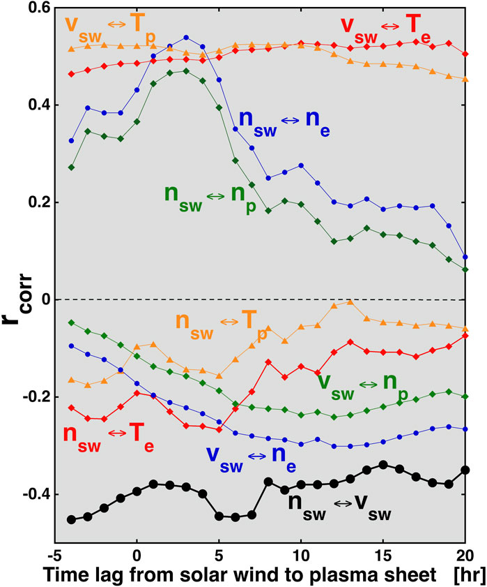
Figure 4. For the central plasma sheet current sheet crossings, the Pearson linear correlations of the plasma sheet densities and temperatures between the solar wind speed and number density are plotted as a function of the time lag between the solar wind and the plasma sheet.

In Figure 4, the Pearson linear correlation coefficients between the central plasma sheet electron and ion number densities and temperatures, and n_sw(t) and v_sw(t), are plotted versus the time lag between the solar wind at Earth and the central plasma sheet measurements. The top four curves of Figure 4 demonstrate that v_sw is positively correlated with the ion and electron temperatures of the central plasma sheet and that n_sw is positively correlated with the ion and electron number densities of the central plasma sheet. The curves also show that the values of the correlation coefficients r_corr depend on the time shift between the solar wind data and the magnetotail current sheet crossing data. The curves at the bottom of Figure 4 demonstrate an opposite, but not as strong, anticorrelation between the solar wind velocity and the central plasma sheet number densities and between the solar wind number density and the central plasma sheet temperatures (See also Rows 5–8 of Table 2). The correlation values r_corr also depend on the time shifts between the two data sets. The black curve at the bottom of Figure 4 points out the robust (time-shifted) anticorrelation between the solar wind number density and the solar wind velocity.

The solar wind number density versus the plasma sheet number density curves in the top of Figure 4 display a narrow peak in the correlation magnitude, an indication of a time-lagged transport timescale from the solar wind into the central plasma sheet for plasma entry (For more evidence of this, see Figure 16 of Borovsky et al. (1998a), Figure 3 of Wing et al. (2006), and Figure 5 and Figures 6–8 of Denton and Borovsky (2009)). The two solar wind velocity versus central plasma sheet temperature curves at the top of Figure 4 do not show an identifiable strong peak in the correlation magnitude, probably owing to the long autocorrelation time of the solar wind velocity.

In addition to regular Pearson linear correlations (PLC) between two time-dependent variables, two other correlation methods are employed, and the results are posted in Table 2: (1) multivariate linear correlations (MLC) between the pair of variables n_s+3 and v_sw+4 and the individual variables n_e, T_e, n_i, and T_i and (2) canonical correlation analysis (CCA) between the time-dependent solar wind state vector (n_sw+3,v_sw+4) and the plasma sheet state vectors (n_e,T_e), (n_i,T_i) (n_e,n_i), and (T_e,T_i) at the times of the current sheet crossings.

In Rows 1–8 of Table 2, PLC is used to correlate one variable with another variable: these rows will be used as baselines for discussion about the use of MLC and CCA. Because the number densities and temperatures of the central plasma sheet are both correlated with the density and speed of the solar wind (e.g., Figures 3, 4), one can ask whether both of those solar wind variables contribute unique information about the description and prediction of the plasma sheet temperatures and densities. Multivariate linear correlation (MLC) is utilized for more information. MLC appears in Rows 9–12 of Table 2. The “Solar wind variables” column for those rows in Table 2 contains the optimal formulae for the linear combination of the two solar wind variables, where the two variables are in standardized form in the formulae. (Standardizing a variable is accomplished by subtracting the mean value of the variable and then dividing by its standard deviation). The Pearson linear correlation between the “Solar wind variables” and the “Central plasma sheet variables” appears in the column labeled “r_corr.” To perform the MLC, only events that contain data for all of the variables can be used. For those same events, the maximum correlation coefficient between a single solar wind variable and a single plasma sheet variable appears in the column labeled “Maximum r_conn of 2 variables.” In Row 1 of Table 2, n_e and n_sw+3 have a correlation coefficient r_corr = 0.542. In Row 9, with the addition of the variable v_sw+4, the correlation remains at 0.542. One could conclude that there is no relevant information contained in v_sw+4 that adds any information to the information already contained in n_sw+3 about the behavior of n_e. Looking at Row 10 of Table 2, it can be seen that adding n_sw+3 to the v_sw+4 versus T_e correlation increases r_corr from 0.493 to 0.497: here, n_sw+3 adds new information about the behavior of T_e, but what n_sw+3 adds is not much more than what v_sw+4 already contains. The “difference” column in Table 2 is the change in the correlation coefficient obtained by adding this new information: for Row 10, this difference is 0.004, which is statistically insignificant. In Row 11, with the addition of the variable v_sw+4, the correlation changes to 0.476 from 0.476. The difference in the correlation is 0.000. Similar to the case of Row 9, one could conclude that there is no relevant information contained in v_sw+4 that adds to the information already contained in n_sw+3 about the behavior of n_i. Looking at Row 12 of Table 2, it is seen that adding n_sw+3 to the v_sw+4 versus T_i correlation does not increase r_corr. Here, n_sw+3 does not add any information about the behavior of T_i. We know that n_sw describes n_e and n_i to a good degree and that v_sw describes T_e and T_i to a good degree. Two conclusions of the MLC analysis are (1) that knowledge of n_sw does not improve the description of the plasma sheet temperatures and (2) that knowledge of v_sw does not improve the description of the plasma sheet densities.

As a note, the information added by a new second variable to a first variable can act in two manners, “suppression” and “confounding” (Conger, 1974; Robins, 1989; Tzelgov and Henik, 1991 Frank, 2000), to increase the correlation coefficient with a target variable: (1) the new added variable can carry additional information about the way the target variable works or (2) the new added variable can carry information about noise in the first variable and the linear combination can act to counteract some of the noise in the original first variable.

Canonical correlation analysis (CCA) appears in Rows 13–16 of Table 2. CCA is a method that finds correlation patterns between one set of variables and a second set of variables (Muller, 1982; Johnson and Wichern, 2007; Gatignon, 2010; Nimon et al., 2010; Borovsky, 2014). These sets of variables can be, for instance, a time-dependent solar wind state vector and a time-dependent central plasma sheet state vector. In these time-dependent problems, we have referred to the CCA process as “vector–vector correlations” (Borovsky, 2014; Borovsky and Denton, 2014, 2018; Borovsky and Osmane, 2019; Borovsky and Lao, 2023). The CCA mathematical scheme reduces each of the two time-dependent state vectors into a time-dependent scalar. Pairs of scalars are produced that are guaranteed to have the highest possible Pearson linear correlation coefficient, r_corr, between them.

In the present study, very simple state vectors are used in Rows 13–16: the solar wind state vector (n_sw+3,v_sw+4) and the plasma sheet state vectors (n_e,T_e), (n_i,T_i), (n_e,n_i), and (T_e,T_i). CCA calculates optimal linear combinations of the state vector variables in standardized form: those linear combinations appear in Rows 13–16 of Table 2. The Pearson linear correlation coefficients between the two linear combinations (solar wind versus plasma sheet) are listed in the “r_corr” column, and the maximum two-variable correlation coefficient for the available events that have data for all of the variables appears in the next column. As can be seen for the four CCA calculations, the differences are not statistically significant: the maximum improvement over the two-variable PLC correlations is an increase of 0.016 in the correlation coefficient (Row 13).

When CCA selects the combinations of solar wind variables and of plasma sheet variables that have the highest possible correlations in the combination of the solar wind-variables (n_sw+3,v_sw+4) with the plasma sheet variables (ne,Te) (Row 13), CCA picks n_sw+3 and n_e with the largest coefficients in the optimal formulae, and they are the two variables that have the highest correlation (column labeled “Maximum r_corr of 2 variables”). In the combination of the solar wind variables (n_sw+3,v_sw+4) with the plasma sheet variables (n_i,T_i) (Row 14), CCA selects v_sw+4 and T_i with the largest coefficients in the optimal formulae and with the largest two-variable correlation. For the plasma sheet number density (Row 15) with (n_sw+3,v_sw+4) versus (n_e,n_i), CCA selects n_sw+3 and n_e as the two variables with the largest coefficients and largest correlation and for plasma sheet temperatures (Row 16) with (n_sw+3,v_sw+4) versus (T_e,T_i) CCA picks v_sw+4 and T_i as the variables with the largest coefficients and the largest two-variable correlation.

As was the case for the MLC calculations, applying CCA gives the impression that the two problems, (a) n_sw driving number densities of the plasma sheet and (b) v_sw driving the temperatures of the plasma sheet, are unrelated to each other.

5 Conclusions, discussions, and future work

In this study, THEMIS-A and THEMIS-B ion and electron number densities n_i and n_e and ion and electron temperatures T_i and T_e measured at current sheet crossings in the Earth’s magnetotail from 10.8 R_E to 76.9 R_E distance downtail were correlated with solar wind number densities n_sw and speeds v_sw at Earth. The current sheet crossings were used to ensure that the THEMIS data were taken from the central plasma sheet at the furthest distances from Earth of closed magnetic flux tubes.

The n_sw versus n_e and n_i correlations are higher at higher values of geomagnetic activity as measured by Hp60, whereas the v_sw versus T_e and T_i correlations are weaker at higher values of Hp60. The n_sw versus n_e and n_i correlations and the v_sw versus T_e and T_i correlations are all of similar strength, except for the v_sw ↔ T_i correlation, which is weak but has very few data points to make that judgment.

Various methods of correlations support the view that n_sw controls n_i and n_e and that v_sw controls T_i and T_e:

• Multivariate linear correlation indicates that supplying information about n_sw does not add significant information to the v_sw ↔ T_i and v_sw ↔ T_e correlations that the variable v_sw does not already contain.

• Likewise, multivariate linear correlation indicates that supplying information about v_sw does not add significant information to the n_sw ↔ n_i and n_sw ↔ n_e correlations that the variable n_sw does not already contain.

• The interpretation of canonical correlation analysis (CCA) is that the n_sw → n_e problem and the v_sw →T_e problem are independent of each other. Likewise, the interpretation of CCA analysis is that the n_sw → n_i problem and the v_sw →T_i problem are independent of each other. This is the case even though v_sw and n_sw have strong anticorrelations with each other.

It seems clear that the n_sw ↔ n_e and n_sw ↔ n_i correlations represent a time-lagged entry of solar wind plasma into the magnetosphere (Cf. Wing et al. (2014) for a review of possible entry physical mechanisms). These correlation conclusions are backed up by the multiple case studies of Borovsky et al. (1998a) and Denton and Borovsky (2009). Less clear is the physical interpretation of the v_sw ↔ T_e and v_sw ↔ T_i correlations, with no clear maximum in the correlation coefficients versus lag time between the solar wind and magnetospheric data sets. One problem, of course, is the very long autocorrelation time for the solar wind speed v_sw. However, in some cases, the optimal correlation coefficient has T_e(t) or T_i(t) leading v_sw(t) in time rather than lagging it in time (not shown in Tables 1, 2). This is probably caused by adiabatic compression of the solar wind as faster solar wind runs into slower solar wind to form a heated compression region ahead in time (as seen by Earth) of the faster solar wind (cf. Figure 4B of Borovsky (2018)). Here, the magnetosheath is hotter before the fast solar wind arrives. Other mechanisms associating plasma sheet temperature with v_sw could be Earthward adiabatic convection of plasma sheet material (Borovsky et al., 1998b) and heating during substorms (Forsyth et al., 2014). In Figure 5A, the logarithms of the ion and electron temperatures of the central plasma sheet for the 1017 current sheet crossings are plotted as a function of the logarithm of the downtail distance |X| in R_E. Note that the ion temperature T_i and the electron temperature T_e have similar downtail profiles, indicating perhaps similar adiabatic heating mechanisms during transport toward the Earth. Borovsky et al. (1998b) found that for ions, the specific entropy was almost conserved in this multi-hour Earthward transport until the dipolar region is reached, where gradient-and-curvature drifts start to move the ion plasma sheet toward the duskside magnetopause. Other plasma sheet heating may be associated with the temporal pressure increases associated with (a) sudden increases in the ram pressure of the solar wind (Borovsky, 1998a) or pressure increases associated with increasing loading of magnetic field into the magnetotail by dayside reconnection (Forsyth et al., 2014). In Figure 5B, the ion-to-electron temperature ratio T_i/T_e in the central plasma sheet is plotted as a function of the downtail distance |X|. The linear-regression line in that plot shows that the more-distant ratio is about a factor of 2 higher than it is in the |X| ∼ 15 R_E range. This may be an indication of different evolutions for the ion temperature versus electron temperature; however, the temperature change with distance in Figure 5A is much greater than the T_i/T_e change in Figure 5B.

Figure 5

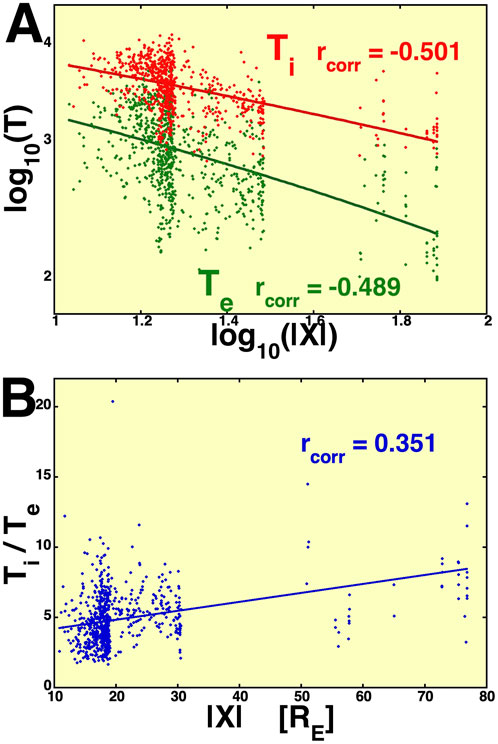
Figure 5. For the central plasma sheet current crossings, Panel (A) plots the logarithms of the ion temperature (red) and the electron temperature (green) as a function of the logarithm of the downtail distance of the crossing, and Panel (B) plots the temperature ratio T_i/T_e as a function of the downtail distance.

Future studies accounting for the time history of the solar wind and the reaction of the plasma sheet are needed. In particular, the use of time integrals of the solar wind number densities, plus a temporal gap after the time integral to account for transport times, is needed for the central plasma sheet number density studies. As noted in Borovsky et al. (1998a) and Denton and Borovsky (2009), there are significant transport times between the solar wind and the various locations in the plasma sheet.

A more extensive CCA analysis of n_e, n_i, T_e, and T_i must be performed using a much larger set of solar wind variables beyond n_sw and v_sw and using independent time lags for the various solar wind variables. With only 1017 current sheet crossings in the magnetotail, physical interpretation of this more extensive CCA analysis will be difficult, but the analysis should lead to clues about other solar wind variables that are important for the densities and temperatures of the central plasma sheet.

Finally, the authors plan to perform correlation studies of the energetic particle populations of the central plasma sheet at the 1017 crossings to discern which properties and which particle populations of the solar wind may be driving the plasma sheet energetic particle populations. Of particular interest is the role of the energetic field-aligned electron strahl in the solar wind at Earth (Borovsky and Runov, 2022).

Data availability statement

The THEMIS ion and electron data with 3-s time resolution is available at CDAWweb (https://cdaweb.gsfc.nasa.gov) as is the THEMIS 3-s magnetic-field data. The solar-wind and Kp data is available from OMNIweb (https://omniweb.gsfc.nasa.gov) and the HP60 index is available at ftp://ftp.gfz-potsdam.de/pub/home/obs/Hpo. The list of current-sheet crossings for THEMIS-B and THEMIS-C is available at Zenodo at https://zenodo.org/records/16340531?token=eyJhbGciOiJIUzUxMiJ9.eyJpZCI6ImQxZTlhMzJjLTAwODgtNGU1Ny1iYzcyLWM3OTA5NjQ5NzgxMiIsImRhdGEiOnt9LCJyYW5kb20iOiJiZDhmODFmM2EzODA4YTdiMGYxYTM1MDUxZTFkOTkzMCJ9.qAHILDOYPTS7fqPBrWUnikh0NwxBDTo-F6DRSZF9RrijHLZ0ZpveIntzzIvAJaaExeoyrUjJ2lujre_nWsCxEQ.

Author contributions

JE: Writing – review and editing, Validation, Conceptualization, Investigation, Funding acquisition, Methodology, Supervision, Resources, Formal Analysis, Software, Writing – original draft, Visualization, Project administration, Data curation. JB: Writing – review and editing, Funding acquisition, Writing – original draft.

Funding

The author(s) declare that financial support was received for the research and/or publication of this article. JE was supported by a VELA Scholarship at the Los Alamos Space Weather Summer School, by the Fulbright Foreign Student Program “Equal Opportunity Scholarship (Beca Igualdad de Oportunidades, BIO 2022)” from the National Agency for Research and Development (ANID), Government of Chile, and by the Fulbright Chile Commission. Additional support for JE was provided by faculty startup funds from Professor Jacob Bortnik through the Department of Atmospheric and Oceanic Sciences (AOS) at the University of California, Los Angeles (UCLA). JEB was supported at the Space Science Institute by the NASA LWS Program via grant 80NSSC23, by the NSF Magnetospheric Program via grant AGS-2149822, and by the NASA HERMES Interdisciplinary Science Program via grant 80NSSC21K1406.

Acknowledgments

The authors thank Andrei Runov for critical help with the THEMIS particle data, and the authors thank Trinidad Duran for helpful discussions and for sharing useful resources on canonical correlation analysis.

Conflict of interest

The authors declare that the research was conducted in the absence of any commercial or financial relationships that could be construed as a potential conflict of interest.

The author(s) declared that they were an editorial board member of Frontiers, at the time of submission. This had no impact on the peer review process and the final decision.

Generative AI statement

The author(s) declare that no Generative AI was used in the creation of this manuscript.

Any alternative text (alt text) provided alongside figures in this article has been generated by Frontiers with the support of artificial intelligence and reasonable efforts have been made to ensure accuracy, including review by the authors wherever possible. If you identify any issues, please contact us.

Publisher’s note

All claims expressed in this article are solely those of the authors and do not necessarily represent those of their affiliated organizations, or those of the publisher, the editors and the reviewers. Any product that may be evaluated in this article, or claim that may be made by its manufacturer, is not guaranteed or endorsed by the publisher.

References

Auster, A. U., Glassmeier, K. H., Magnes, W., Aydogar, O., Baumjohann, W., Constantinescu, D., et al. (2008). The THEMIS fluxgate magnetometer. Space Sci. Rev. 141, 235–264. doi:10.1007/s11214-008-9365-9

CrossRef Full Text | Google Scholar

Bame, S. J., Asbridge, J. R., Felthauser, H. E., Olsen, R. A., and Strong, I. B. (1966). Characteristics of the plasma sheet in the Earth's magnetotail. J. Geophys. Res. 72, 113. doi:10.1029/jz072i001p00113

CrossRef Full Text | Google Scholar

Bame, S. J., Asbridge, J. R., Felthauser, H. E., Hones, E. W., and Strong, I. B. (1967). Electrons in the plasma sheet of the Earth's magnetic tail. Phys. Rev. Lett. 16, 138–142. doi:10.1103/physrevlett.16.138

CrossRef Full Text | Google Scholar

Baumjohann, W. (1993). The near-Earth plasma sheet: an AMPTE/IRM perspective. Space Sci. Rev. 64, 141–163. doi:10.1007/BF00819660

CrossRef Full Text | Google Scholar

Bendat, J. S., and Piersol, A. G. (2010). Random data: analysis and measurement procedures. 4th edition. New York: John Wiley, 99–102.

Google Scholar

W. H. Beyer (1966). Handbook of tables for probability and statistics (Cleveland, Ohio: Chem. Rubber), IX.

Google Scholar

Borovsky, J. E. (2014). Canonical correlation analysis of the combined solar-wind and geomagnetic-index data sets. J. Geophys. Res. 119, 5364–5381. doi:10.1002/2013ja019607

CrossRef Full Text | Google Scholar

Borovsky, J. E. (2018). On the origins of the intercorrelations between solar wind variables. J. Geophys. Res. 123, 20–29. doi:10.1002/2017ja024650

CrossRef Full Text | Google Scholar

Borovsky, J. E., and Denton, M. H. (2006). The differences between CME-driven storms and CIR-driven storms. J. Geophys. Res. 111, A07S08. doi:10.1029/2005JA011447

CrossRef Full Text | Google Scholar

Borovsky, J. E., and Denton, M. H. (2014). Exploring the cross-correlations and autocorrelations of the ULF indices and incorporating the ULF indices into the systems science of the solar-wind-driven magnetosphere. J. Geophys. Res. 119, 4307–4334. doi:10.1002/2014ja019876

CrossRef Full Text | Google Scholar

Borovsky, J. E., and Denton, M. H. (2018). Exploration of a composite index to describe magnetospheric activity: reduction of the magnetospheric state vector to a single scalar. J. Geophys. Res. 123, 7384–7412. doi:10.1029/2018ja025430

CrossRef Full Text | Google Scholar

Borovsky, J. E., and Lao, C. J. (2023). A system science methodology develops a new composite highly-predictable index of magnetospheric activity for the community: the whole-earth index E₍₁₎. Front. Astron. Space Sci. 10, 1214804. doi:10.3389/fspas.2023.1214804

CrossRef Full Text | Google Scholar

Borovsky, J. E., and Osmane, A. (2019). Compacting the description of a time-dependent multivariable system and its multivariable driver by reducing the state vectors to aggregate scalars: the Earth's solar-wind-driven magnetosphere. Nonlin. Process. Geophys. 26, 429–443. doi:10.5194/npg-26-429-2019

CrossRef Full Text | Google Scholar

Borovsky, J. E., and Runov, A. (2022). Is the solar wind electron strahl a seed population for the Earth’s electron radiation belt? Front. Astron. Space Sci. 9, 930162. doi:10.3389/fspas.2022.930162

CrossRef Full Text | Google Scholar

Borovsky, J. E., and Steinberg, J. T. (2006). The “calm before the storm” in CIR/magnetosphere interactions: occurrence statistics, solar-wind statistics, and magnetospheric preconditioning. J. Geophys. Res. 111, A07S10. doi:10.1029/2005ja011397

CrossRef Full Text | Google Scholar

Borovsky, J. E., and Valdivia, J. A. (2018). The Earth’s magnetosphere: a systems science overview and assessment. Surv. Geophys 39, 817–859. doi:10.1007/s10712-018-9487-x

PubMed Abstract | CrossRef Full Text | Google Scholar

Borovsky, J. E., and Yakymenko, K. (2017). Systems science of the magnetosphere: creating indices of substorm activity, of the substorm-injected electron population, and of the electron radiation belt. J. Geophys. Res. 122, 10012. doi:10.1002/2017ja024250

CrossRef Full Text | Google Scholar

Borovsky, J. E., Thomsen, M. F., and Elphic, R. C. (1998a). The driving of the plasma sheet by the solar wind. J. Geophys. Res. 103, 17617–17639. doi:10.1029/97ja02986

CrossRef Full Text | Google Scholar

Borovsky, J. E., Thomsen, M. F., Elphic, R. C., Cayton, T. E., and McComas, D. J. (1998b). The transport of plasma-sheet material from the distant tail to geosynchronous orbit. J. Geophys. Res. 103, 20297–20331. doi:10.1029/97ja03144

CrossRef Full Text | Google Scholar

Conger, A. J. (1974). A revised definition for suppressor variables: a guide to their identification and interpretation. Educ. Psychol. Meas. 34, 35–46. doi:10.1177/001316447403400105

CrossRef Full Text | Google Scholar

Denton, M. H., and Borovsky, J. E. (2009). The superdense plasma sheet in the magnetosphere during high-speed-stream-driven storms: plasma transport timescales. J. Atmos. Solar-Terr. Phys. 71, 1045–1058. doi:10.1016/j.jastp.2008.04.023

CrossRef Full Text | Google Scholar

Dubyagin, S., Ganushkina, N. Y., Sillanpää, I., and Runov, A. (2016). Solar wind-driven variations of electron plasma sheet densities and temperatures beyond geostationary orbit during storm times. J. Geophys. Res. Space Phys. 121, 8343–8360. doi:10.1002/2016ja022947

CrossRef Full Text | Google Scholar

Echera, E., Gonzalez, W. D., Gonzalez, A. L. C., Prestes, A., Vieira, L. E. A., Dal Lago, A., et al. (2004). Long-term correlation between solar and geomagnetic activity. J. Atmos. Solar-Terrestrial Phys. 66, 1019–1025. doi:10.1016/j.jastp.2004.03.011

CrossRef Full Text | Google Scholar

Fairfield, D. H. (1971). Average and unusual locations of the Earth's magnetopause and bow shock. J. Geophys. Res. 28, 6700–6716. doi:10.1029/ja076i028p06700

CrossRef Full Text | Google Scholar

Frank, K. A. (2000). Impact of a confounding variable on a regression coefficient. Sociological Meth. Res. 29, 147. doi:10.1177/0049124100029002001

CrossRef Full Text | Google Scholar

Forsyth, C., Watt, C. E. J., Rae, I. J., Fazakerley, A. N., Kalmoni, N. M. E., Freeman, M. P., et al. (2014). Increases in plasma sheet temperature with solar wind driving during substorm growth phases. Geophys. Res. Lett. 41, 8713–8721. doi:10.1002/2014gl062400

PubMed Abstract | CrossRef Full Text | Google Scholar

Gatignon, H. (2010). Statistical analysis of management data. New York: Springer.

Google Scholar

Greenstadt, E. W., Traver, D. P., Coroniti, F. V., Smith, E. J., and Slavin, J. A. (1990). Observations of the flank of Earth's bow shock to −110 R_E by ISEE 3/ICE. Gephys. Res. Lett. 17, 753–756. doi:10.1029/gl017i006p00753

CrossRef Full Text | Google Scholar

Hones, E. W., Asbridge, J. R., and Bame, S. J. (1971). Time variations of the magnetotail plasma sheet at 18 R_E determined from concurrent observations by a pair of Vela satellites. J. Geophys. Res. 76, 4402–4419. doi:10.1029/ja076i019p04402

CrossRef Full Text | Google Scholar

Johnson, R. A., and Wichern, D. W. (2007). Applied multivariate statistical analysis. 6th Ed. Upper Saddle River, New Jersey: Pearson Prentice Hall.

Google Scholar

Kennel, C. F. (1988). Shock structure in classical magnetohydrodynamics. J. Geophys. Res. 93, 8545–8557. doi:10.1029/ja093ia08p08545

CrossRef Full Text | Google Scholar

Kronberg, E. A., Ashour-Abdalla, M., Dandouras, I., Delcourt, D. C., Grigorenko, E. E., Kistler, L. M., et al. (2014). Circulation of heavy ions and their dynamical effects in the magnetosphere: recent observations and models. Space Sci. Rev. 184, 173–235. doi:10.1007/s11214-014-0104-0

CrossRef Full Text | Google Scholar

Lavraud, B., Thomsen, M. F., Wing, S., Fujimoto, M., Denton, M. H., Borovsky, J. E., et al. (2006a). Observation of two distinct cold, dense ion populations at geosynchronous orbit: local time asymmetry, solar wind dependence and origin. Ann. Geophys. 24, 3451–3465. doi:10.5194/angeo-24-3451-2006

CrossRef Full Text | Google Scholar

Lavraud, B., Thomsen, M. F., Lefebvre, B., Schwartz, S. J., Seki, K., Phan, T. D., et al. (2006b). Evidence for newly closed magnetosheath field lines at the dayside magnetopause under northward IMF. J. Geophys Res. 111, A05211. doi:10.1029/2005ja011266

CrossRef Full Text | Google Scholar

Lavraud, B., Borovsky, J. E., Genot, V., Schwartz, S. J., Birn, J., Fazakerley, A. N., et al. (2009). Tracing solar wind plasma entry into the magnetosphere using ion-to-electron temperature ratio. Geophys. Res. Lett. 36, L18109. doi:10.1029/2009gl039442

CrossRef Full Text | Google Scholar

Lennartsson, W., and Shelley, E. G. (1986). Survey of 0.1- to 16-keV/e plasma sheet ion composition. J. Geophys. Res. 91, 3061–3076. doi:10.1029/ja091ia03p03061

CrossRef Full Text | Google Scholar

Lin, R. L., Zhang, X. X., Liu, S. Q., Wang, Y. L., and Gong, J. C. (2010). A three-dimensional asymmetric magnetopause model. J. Geophys. Res. 115, A04207. doi:10.1029/2009ja014235

CrossRef Full Text | Google Scholar

McFadden, J. P., Carlson, C. W., Larson, D., Ludlam, M., Abiad, R., Elliott, B., et al. (2008). The THEMIS ESA plasma instrument and in-flight calibration. Space Sci. Rev. 141, 277–302. doi:10.1007/s11214-008-9440-2

CrossRef Full Text | Google Scholar

Muller, K. E. (1982). Understanding canonical correlation through the general linear model and principal components. Amer. Stat. 36, 342–354. doi:10.1080/00031305.1982.10483045

CrossRef Full Text | Google Scholar

Nimon, K., Henson, R. K., and Gates, M. S. (2010). Revisiting interpretation of canonical correlation analysis: a tutorial and demonstration of canonical commonality analysis. Multivar. Behav. Res. 45, 702–724. doi:10.1080/00273171.2010.498293

PubMed Abstract | CrossRef Full Text | Google Scholar

Phan, T.-D., Paschmann, G., Baumjohann, W., Sckopke, N., and Luhr, H. (1994). The magnetosheath region adjacent to the dayside magnetopause: AMPTE/IRM observations. J. Geophys. Res. 99, 121–141. doi:10.1029/93JA02444

CrossRef Full Text | Google Scholar

Robins, J. (1989). The control of confounding by intermediate variables. Stat. Medicine 8, 679.

PubMed Abstract | CrossRef Full Text | Google Scholar

Terasawa, T., Fujimoto, M., Mukai, T., Saito, Y., Yamamoto, T., Machida, S., et al. (1997). Solar wind control of density and temperature in the near-Earth plasma sheet: WIND/GEOTAIL collaboration. Geophys. Res. Lett. 24, 935–938. doi:10.1029/96gl04018

CrossRef Full Text | Google Scholar

Thomsen, M. F., Borovsky, J. E., Skoug, R. M., and Smith, C. W. (2003). Delivery of cold, dense plasma sheet material into the near-Earth region. J. Geophys. Res. 108, 2002JA009544. doi:10.1029/2002ja009544

CrossRef Full Text | Google Scholar

Tsyganenko, N. A., and Mukai, T. (2003). Tail plasma sheet models derived from Geotail particle data. J. Geophys. Res. Space Phys. 108. doi:10.1029/2002ja009707

CrossRef Full Text | Google Scholar

Tzelgov, J., and Henik, A. (1991). Suppression situations in psychological research: definitions, implications, and applications. Psychol. Bull. 109, 524–536. doi:10.1037//0033-2909.109.3.524

CrossRef Full Text | Google Scholar

Walsh, A. P., Haaland, S., Forsyth, C., Keeese, A. M., Kissinger, J., Li, K., et al. (2014). Dawn–dusk asymmetries in the coupled solar wind–magnetosphere–ionosphere system: a review. Ann. Geophys. 32, 705–737. doi:10.5194/angeo-32-705-2014

CrossRef Full Text | Google Scholar

Wang, C.-P., Gkioulidou, M., Lyons, L. R., and Angelopoulos, V. (2012). Spatial distibution of the ion and electron temperature ratio in the magnetosheath and plasma sheet. J. Geophys. Res. 117, A08215. doi:10.1029/2012JA017658

CrossRef Full Text | Google Scholar

Wing, S., and Newell, P. T. (2002). 2D plasma sheet ion density and temperature profiles for northward and southward IMF. Geophys. Res. Lett. 29. doi:10.1029/2001gl013950

CrossRef Full Text | Google Scholar

Wing, S., Johnson, J. R., and Fujimoto, M. (2006). Timescale for the formation of the cold-dense plasma sheet: a case study. Geophys. Res. Lett. 33, L23106. doi:10.1029/2006gl027110

CrossRef Full Text | Google Scholar

Wing, S., Ohtani, S., Johnson, J., Wilson, G. R., and Higuchi, T. (2014). Field-aligned currents during the extreme solar minimum between the solar cycles 23 and 24. J. Geophys. Res. Space Phys. 119, 2466–2475. doi:10.1002/2013JA019452

CrossRef Full Text | Google Scholar

Yan, G. W., Shen, C., Liu, Z. X., Carr, C. M., Rème, H., and Zhang, T. L. (2005). A statistical study on the correlations between plasma sheet and solar wind based on DSP explorations. Ann. Geophys. 23, 2961–2966. doi:10.5194/angeo-23-2961-2005

CrossRef Full Text | Google Scholar

Young, D. T., Balsiger, H., and Geiss, J. (1982). Correlations of magnetospheric ion composition with geomagnetic and solar activity. J. Geophys. Res. 87, 9077–9096. doi:10.1029/ja087ia11p09077

CrossRef Full Text | Google Scholar

Yu, Y., Chen, Z., and Chen, F. (2020). Cold and dense plasma sheet caused by solar wind entry: direct evidence. Atmosphere 831, 831. doi:10.3390/atmos11080831

CrossRef Full Text | Google Scholar