Vertical damping of gravity waves evaluated from ACS-TGO solar occultation measurements on Mars

Amplitudes of gravity waves generated in the lower and denser atmospheric layers grow exponentially with height as they propagate to the upper and thinner atmosphere, where they are reduced by various processes. Their vertical decay is accompanied by a transfer of wave momentum and energy to the ambient flow, which represents a significant force in the upper atmosphere. Constraining the vertical damping and elucidating the related mechanisms are crucial for understanding the dynamics. Previous observations of gravity waves in the Martian thermosphere by different instruments provided evidence that amplitudes of relative temperature disturbances are inversely proportional to the mean temperature. This suggests that wave amplitudes may be limited by convective instabilities. However, this anticorrelation was not observed at all heights or in all measurements, sparking a discussion about the dominant mechanisms of wave damping. Using vertical temperature profiles collected by the Atmospheric Chemistry Suite instrument on board Trace Gas Orbiter over more than 6 years, we examined the statistical behavior of wave amplitudes and their vertical damping rates. We found a weak anticorrelation near the mesopause ($\sim$90–140 km), suggesting the presence of convective instability and molecular diffusion mechanisms, but no robust correlations elsewhere. Instead, we found an unexpectedly persistent anticorrelation between the vertical decay rates and ambient temperature at all heights. We demonstrated that above approximately 80 km, wave breaking and/or saturation could be consistent with the convective instability mechanism, but the reason for this behavior at lower altitudes remains unclear.

1 Introduction

Gravity waves (GWs) are maintained by a balance of two forces: gravity and buoyancy. Therefore, they are a common feature of all convectively stable planetary atmospheres (e.g., see reviews by Medvedev and Yiğit (2019); Yiğit and Medvedev (2019)). These waves redistribute energy, heat and momentum across vertical layers, thus playing an important role in the dynamics of the middle and upper atmospheres. Characterizing the GW fields is therefore essential for understanding the dynamics and constraining GW parameterizations in numerical general circulation models, thereby improving their predictive capabilities.

Numerous observations performed from Martian orbiters have provided a substantial amount of information about GWs in the atmosphere of Mars. One challenging and debatable topic that arose from these observations is the relationship between average wave amplitudes and the mean ambient temperature. The first indication of an anticorrelation between magnitudes of the relative ${\text{CO}}_2$ density fluctuations (i.e., normalized by the mean density), and temperature was reported by Yiğit et al. (2015), (Figure 2b) based on a limited set of measurements taken with the Neutral Gas and Ion Mass Spectrometer (NGIMS) instrument on board the Mars Atmosphere and Volatile EvolutioN (MAVEN) satellite in the upper thermosphere. Using a longer NGIMS dataset, Terada et al. (2017) and England et al. (2017) corroborated this finding and suggested that the anticorrelation is dictated by saturation processes in isothermal conditions at the exobase. A similar relationship was found in the MAVEN data by Siddle et al. (2019) and Leelavathi et al. (2020), except during the global dust storm of 2018.

In addition to MAVEN’s measurements in the upper thermosphere, Vals et al. (2019) analyzed density fluctuations in the lower thermosphere obtained from accelerometers during the aerobraking phases of other orbiters: Mars Global Surveyor, Mars Odyssey, and Mars Reconnaissance Orbiter. In the more general case where the background temperature varies with height, the saturation condition based on the convective instability threshold converts to proportionality between the relative wave perturbation amplitudes and the squared Brunt-Väisälä frequency $N^2$ (Fritts et al., 1988, Equation 6). Vals et al. (2019) identified this correlation in some datasets and in certain places, but not for all orbiters or at all latitudes. Similarly, Jesch et al. (2019) did not find an anticorrelation between the amplitudes of relative temperature disturbances and mean temperature in ExoMars Trace Gas Orbiter (TGO) accelerometer data. Then, the study of Starichenko et al. (2021) did not reveal a positive correlation with $N^2$ at all heights in the retrievals performed by the Atmospheric Chemistry Suite (ACS) instrument onboard this spacecraft. These results suggest that convective instability is not the only process shaping the GW amplitudes in the middle and upper atmosphere. Other physical mechanisms may also be at work.

An increase in the background temperature alters not only static stability, but also dissipation and density. Both molecular diffusion and heat conduction increase with temperature, resulting in stronger wave damping, furthermore higher temperatures reduce the rate of vertical amplitude growth by extending the atmosphere and increasing the scale height (Yiğit and Medvedev, 2010). Theoretical estimates show that on Mars, the latter dominates the former up to 160–180 km (Yiğit et al., 2021b; Figure 11b).

In this paper, we apply the ACS-TGO dataset of temperature profiles, covering altitudes between 10 and maximum 180 km, with high enough vertical resolution to study the physical processes that affect the propagation and vertical decay of GWs. The temperature profiles were previously retrieved from the ACS solar occultations as described by (Belyaev et al., 2022; Fedorova et al., 2023) and analyzed for GWs by Starichenko et al. (2021), Starichenko et al. (2024). Now, the statistics of profiles with the GW characteristics is extended from the second half of the Martian year 34 (MY34) up to the end of MY37.

2 Methods

2.1 Retrievals of temperature profiles

ACS is a set of three spectrometers on board the TGO spacecraft, which is part of the ExoMars 2016 joint campaign between ESA and Roscosmos. The three spectrometers represent the near (NIR; 0.73–1.6 $\mu$m), middle (MIR; 2.3–4.2 $\mu$m) and thermal (TIRVIM; 1.7–17 $\mu$m) infrared channels (Korablev et al., 2018). In our study, we use only the data from the NIR and MIR channels. Both channels work in the solar occultation mode and possess a high spectral resolving power $\sim$25,000, a signal to noise ratio >1,000 and a vertical resolution $\sim$1 km. The MIR channel is a cross-dispersion echelle spectrometer that allows retrieving temperature and density vertical profiles within the 20–180 km altitude range from the strong absorption ${\text{CO}}_2$ band at 2.7 $\mu$m (Belyaev et al., 2021; Belyaev et al., 2022). The NIR channel is another echelle spectrometer combined with an acousto-optic tunable filter for a selection of the diffraction orders. It senses ${\text{CO}}_2$ absorption bands at 1.43 $\mu$m and 1.57 $\mu$m when deriving temperature and density profiles within the 10–100 km range (Fedorova et al., 2020; Fedorova et al., 2023). MIR and NIR instruments can make simultaneous solar occultation measurements, as their lines of sight (LOSs) target the same tangent point, thus allowing for cross-validation. An altitude of the tangent point is considered to be the closest distance between the instrument’s LOS and the areoid planetary surface. The atmospheric transmission spectrum at each observed altitude is calculated as a ratio of the solar spectrum on the LOS transmitted through the atmosphere to the reference solar spectrum measured at an altitude where the ${\text{CO}}_2$ absorption of the chosen band is insignificant. This corresponds to about 200 km for the MIR 2.7 $\mu$m band and 130–150 km for the NIR bands at 1.4–1.6 $\mu$m.

The procedures describing the retrieval of temperature and density profiles from the MIR and NIR measurements are outlined in works of Belyaev et al. (2021), Belyaev et al. (2022) and Fedorova et al. (2020), Fedorova et al. (2023), respectively. At each altitude, the algorithm solves an optimization problem using partial derivatives of transmission spectra on the retrieved parameters. We consider rotational ${\text{CO}}_2$ lines whose absorption cross sections are highly dependent on temperature. Then, the hydrostatic assumption for pressure is applied to the derived temperature and ${\text{CO}}_2$ density profiles, and the retrieval routine is repeated by a few iterations. To remove artificial fluctuations in the vertical profiles between neighboring points, the Tikhonov regularization is used at each iteration step. This avoids high-frequency artifacts, leaving detectable only physical GWs with wavelengths of 4–5 km and longer. The described algorithm was performed for both ACS channels independently, so the retrieved temperature profiles match within 5–10 K (Belyaev et al., 2022).

In the present study, we use the profiles accumulated since the beginning of ACS operations in April 2018, the middle of MY34, till October 2024, the end of MY37. The upper panel of Figure 1 presents the latitude coverage of both MIR and NIR occultations with respect to the solar longitude $L_s$. The dataset is separated by the measurements made in the northern and southern hemispheres. Each dot in the coverage corresponds to one session of occultation, either at the dawn or at the dusk terminators. Observation coordinates are considered with respect to the tangent point that changes during one occultation by less than 2$°$ of latitude. The statistics of the MIR measurements at 2.7 $\mu$m count 1,189 retrieved profiles, while for the NIR ${\text{CO}}_2$ bands it is $\sim$10 times more. In case of simultaneous observations, we use only the MIR data since those profiles cover a broader altitude range than NIR. In the rest of cases, the NIR profiles are used just below 100 km. In Figure 1, the gap in MY37 at $L_s$ = 40$°$-200$°$ corresponds to yet unprocessed transmission spectra.

Figure 1

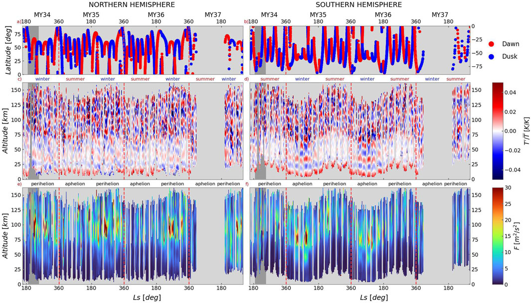
Figure 1. Upper row (a, b): Latitude coverage of ACS measurements as a function of the solar longitude Ls; color indicates the local time of observations. Middle and bottom rows: seasonal-altitude distribution of relative temperature perturbations (c, d) and wave momentum flux (per unit mass) (e, f), correspondingly (shown in color bars). The left (a, c, e) and right (b, d, f) columns present the data for the northern and southern hemispheres, respectively. Gray shaded area denotes the period of global dust storm (GDS). Red dashed lines separate Martian years MY34 to MY37.

2.2 Retrievals of gravity waves and their characteristics

The method for extracting GWs and its characteristics from temperature profiles $T(z)$ was previously described in detail by Starichenko et al. (2021), Starichenko et al. (2024). First, we separate the profile of background temperature $\bar{T}(z)$ from $T(z)$ to derive the difference $T^{\prime }=T-\bar{T}$. For this, we smooth $T(z)$ by cubic polynomials in a sliding window of 60 km width, which is shifted from the bottom to the top of the profile with a step of 7 km and then reverses direction. To obtain a more accurate form of $\bar{T}(z)$ at the top and bottom, the width of the sliding window is gradually reduced to 15 km as it approaches the edges of the profile. Thereafter, all the overlapping polynomials are averaged, and the resulting profile is smoothed using a moving average. For the MIR measurements, intervals of 4 km at the top and the bottom of $\bar{T}(z)$ are cut due to the spurious behavior of the polynomials at the edges. For NIR, we similarly cut 4 km at the bottom and 25 km at the top for better merging with the MIR profiles.

The second and third rows in Figure 1 present the seasonal $(L_s)$ change of altitude profiles for the relative perturbations $T^{\prime }/\bar{T}$ and the vertical flux of horizontal momentum (per unit mass) $F$, correspondingly. The momentum flux is defined as $\mathbf{F}=(F_x,F_y,0)=(\overline{u^{\prime }{w}^{\prime }},\overline{v^{\prime }{w}^{\prime }},0)$, where $u^{\prime }$, $v^{\prime }$ and $w^{\prime }$ are the zonal, meridional and vertical components of wave-induced perturbations of velocity, correspondingly. The direction of the flux cannot be determined from a single profile, but the absolute value of the flux can be evaluated as $F=\sqrt{F_x^2+F_y^2}$ and represented as follows (e.g., Ern et al. (2004); Section 4):

$F={\displaystyle \sum _{k_h,m}}\frac{1}{2}\frac{k_h}{m}{\left(\frac{g}{N}\right)}^2{\left(\frac{|T_{k,m}^{\prime }|}{\bar{T}}\right)}^2.(1)$

The variables $k_h$ and $m$ in Equation 1 are the horizontal and vertical wavenumbers, $|T_{k,m}^{\prime }|$ is the amplitude of the corresponding harmonic, and summation over all $k_h$ and $m$ is done. The wave amplitude $|T^{\prime }|=\sqrt{\overline{T^{\prime 2}}}$ represents the envelope of temperature perturbations in the observed wave packet. It is evaluated by performing a Fourier decomposition within every 60-km sliding window and summing the inputs of all harmonics. In Equation 1, $N$ stands for the Brunt-Väisälä frequency, which characterizes the convective stability of the atmosphere:

$N^2=\frac{g}{T}\left(\frac{dT}{dz}+\frac{g}{c_p}\right),(2)$

where $g$ is the acceleration due to gravity and $c_p$ is the specific heat capacity at constant pressure. If the gradient $-dT/dz$ approaches or exceeds the dry adiabatic lapse rate $g/c_p$, the atmosphere becomes convectively unstable $(N^2\le 0)$ and can no longer support GW propagation. Hence, GWs experience breaking and/or dissipation when the local Brunt-Väisälä frequency is small or negative.

Whereas amplitudes and vertical wavenumbers can be derived from vertical profiles with the help of Fourier analysis, the horizontal wavenumber cannot be determined due to the occultation geometry. Therefore, its value should be prescribed to scale the flux $F$ and provide a meaningful dimension (Starichenko et al., 2024; Section 3). In our case, the value of the horizontal wavelength is taken as ${\lambda }_h^{*}=2\pi /k_h^{*}=300$ km, as this value agrees with the length of the densest atmospheric footprint of 400 km (harmonics with shorter horizontal scales are smoothed over) and the range of values ${\lambda }_h$ = 100–500 km used in GW parameterizations in global circulation models (GCMs) (e.g., Shaposhnikov et al., 2022).

Figure 1 (the second and third rows) shows an increase of wave activity in winters, which was reported also in our previous study based on a shorter dataset (Starichenko et al., 2024). The magnitudes of $F$ in the middle atmosphere are larger and occur lower in the southern hemisphere during aphelion winters, while the peaks extend higher (up and above 100 km) during the perihelion winters. The figure shows that filtering and breaking/saturation processes greatly restrict wave amplitudes in the upper atmosphere. These results are in accordance with previous observational and modeling studies (e.g., Nakagawa et al., 2020; Kuroda et al., 2019; Liu et al., 2023). We will focus on the vertical decay rates in the next sections. Note also the enhancement of wave activity in both hemispheres during the global dust storm of MY34 (gray shaded area), which was predicted using high-resolution general circulation modeling (Kuroda et al., 2020) and detected in the upper thermosphere (Leelavathi et al., 2020; Yiğit et al., 2021a).

3 Results

Our previous study presented linear regressions of the amplitudes of relative temperature disturbances $|T^{\prime }|/\bar{T}$ versus the mean temperature $\bar{T}$ and $N^2$ at certain heights (Starichenko et al., 2021, Section 4.3; Figure 8). No clear correlation was seen, so the conclusion was made that convective instability is not the main mechanism of GW damping. Using the extended dataset, we now revisit this issue by plotting the distribution of $|T^{\prime }|/\bar{T}$ over all heights of the $\bar{T}(z)$ profiles. It is shown in the upper row of Figure 2, where the amplitude $|T^{\prime }|/\bar{T}$ is indicated by colorbars. In this and the next figures, we have grouped individual profiles into 5-km altitude bins and subdivided the data into four $L_s$ seasons. Each panel includes profiles from the entire range of latitudes, since the shown behavior is very similar across all latitude bands. The largest amplitudes of relative temperature disturbances are seen in the mesopause region, especially in the coldest areas with temperatures $\lesssim 140$ K. The anticorrelation is also visible in the surrounding areas. However, there is no clear dependence between $|T^{\prime }|/\bar{T}$ and the mean temperature for the rest of the temperature intervals and altitudes.

Figure 2

Figure 2. Upper row (a–d): relative temperature perturbations as functions of the mean temperature; Middle row (e–h): relative temperature perturbations as a function of the squared Brunt-Väisälä frequency $N^2$; Bottom row (i–l): momentum flux (per unit mass) as a function of the mean temperature and altitude. The four columns represent Martian seasons. First column (a,e,i): $L_s=0\pm 45°$; second (b,f,j): $L_s=90\pm 45°$; third (c,g,k): $L_s=180\pm 45°$; fourth (d, h, l): $L_s=270\pm 45°$.

The saturation mechanism due to convective instability can explain the anticorrelation near the mesopause ($\sim$110–120 km), where $d\bar{T}/dz$ is small. For other altitudes, however, a more general criterion must be applied via the formula (e.g., Fritts et al., 1988, Equation 6):

$\frac{|T^{\prime }|}{\bar{T}}=\frac{|u^{\prime }|}{|c-\bar{u}|}\frac{N^2}{mg},(3)$

where $u^{\prime }$ is amplitude of horizontal velocity disturbances, $c$ is the horizontal phase velocity, $\bar{u}$ is the background wind. The ratio $|u^{\prime }|/|c-\bar{u}|$ approaches a constant of $1/\sqrt{2}\approx 0.7$ at saturation, in accordance with theoretical considerations (Medvedev and Klaassen, 2000) and observational studies (Fritts et al., 1988). Therefore, the amplitudes of relative temperature perturbations have to be directly proportional to $N^2$ at saturation levels, except for small deviations associated with the varying dominant vertical wavenumber $m$ of packets. To verify the hypothesis of saturation due to convective instability, we plotted $|T^{\prime }|/\bar{T}$ as a function of the squared mean Brunt-Väisälä frequency at all altitudes in the middle row of Figure 2 using the same color scale as in the upper row. It shows that the amplitudes are generally larger for large $N^2$, in agreement with the convective instability criterion Equation 3, but the increase is also seen for less stable stratifications (small $N^2$). Moreover, the relative amplitudes weakly depend on $N^2$ above $\sim$80 km for all seasons. This means that the GW distributions cannot be explained entirely by the saturation mechanism associated with convective instability alone.

Further insight into the processes that determine the distribution of GWs can be gained by considering the momentum flux $F$. As a quadratic function of amplitude, it represents the instantaneous distributions. It also characterizes vertical wave propagation and damping, as discussed below. The bottom row of Figure 2 presents the distribution of the calculated fluxes $F$ as a function of the mean temperature and altitude. As expected, the fluxes increase with height in the middle atmosphere in response to the density decrease. They reach their maximum at different altitudes, and decay above, affected by damping. Except for the maxima of $F$ near the cold mesopause region, the figure shows no systematic relationship between the wave activity and background temperature.

4 Discussion

To evaluate the damping of GWs, we consider the net momentum flux $\bar{\rho }F$, where $\bar{\rho }$ is the mean density. This quantity remains constant with height, unless wave dissipation occurs. In the latter case, $d\bar{\rho }F/dz=-\beta \bar{\rho }F$, or, after differentiating and normilizing with respect to $F$ (cf. Yiğit et al. (2021b); Equation 2):

$\frac{dF}{Fdz}=-\frac{d\bar{\rho }}{\bar{\rho }dz}-\beta \equiv \frac{1}{H}-\beta ,(4)$

where $\beta$ is the vertical damping rate, the term $1/H$ characterizes the growth rate due to the density decrease, $H=R\bar{T}/g$ is the density scale height, and $R$ is the specific gas constant. Equation 4 provides a means of directly evaluating the damping rate $\beta$, as the other terms can be derived from observational data.

Figure 3 presents the growth $1/H$ (upper row) and decay $\beta$ (middle row) rates calculated for all profiles shown in Figure 1 as functions of the mean temperature and height. Additionally, the results were subdivided into four seasons. The growth rates vary between approximately 0.1 and 0.175 ${\text{km}}^{-1}$, while the range of $\beta$ is broader, spanning from 0 to 0.3 ${\text{km}}^{-1}$. Since 1/H is inversely proportional to temperature, it is the largest in the coldest mesopause region. The decay rate $\beta$ encompasses all processes that limit wave amplitude growth. They include not only saturation/breaking due to convective instability and dissipation by molecular diffusion and heat conduction, but also filtering by background winds. Figure 3 (middle row) shows that the largest $\beta$ occurs in the mesopause region as well. It significantly exceeds the growth rate of $1/H$, making the mesopause the place of the strongest wave damping. In contrast, the bluish areas below $\sim$100 km in Figures 3e,f,g,h indicate the regions of weak damping where the term $1/H$ exceeds $\beta$, and GW amplitudes grow with height.

Figure 3

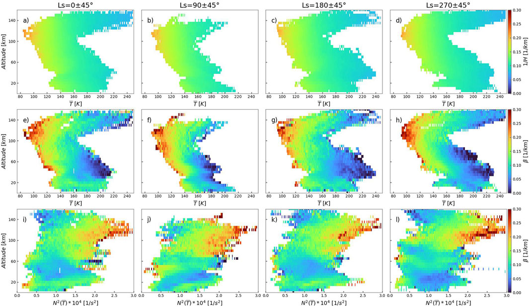
Figure 3. Upper row (a–d): vertical wave growth rate $1/H$ as a function of the mean temperature; Middle row (e–h): wave damping rate $\beta$ as a function of the mean temperature; Bottom row (i–l): Wave damping rate $\beta$ as a function of the squared Brunt-Väisälä frequency $N^2$. The four columns represent Martian seasons: First column (a,e,i) $L_s=0\pm 45°$; second (b,f,j): $L_s=90\pm 45°$; third (c,g,k): $L_s=180\pm 45°$; fourth (d, h, l): $L_s=270\pm 45°$.

It is noteworthy that the damping rate $\beta$ is inversely proportional to the mean temperature at almost all heights. The reason for this is not immediately clear. However, it is known that the damping rate due to molecular diffusion and heat conduction ${\beta }_{\mathit{mol}}$ is proportional to $N^3$ (Yiğit and Medvedev, 2010; Equation 3), while the damping rate associated with nonlinear breaking/saturation ${\beta }_{\mathit{non}}$ is proportional to $N$ (Yiğit and Medvedev, 2010, Equation 5). To determine if these physical processes are involved in limiting the wave amplitude growth, we plotted the calculated $\beta$ as a function of $N^2$ in Figure 3 (bottom row). The plot shows some positive correlation between $\beta$ and the mean Brunt-Väisälä frequency at altitudes above $\sim$80 km and across all seasons. However, it is not possible to determine whether this proportionality is to $N$ or to $N^3$. The lack of the correlation below $\sim$80 km suggests that other unidentified processes may be responsible for the observed anticorrelation between $\beta$ and temperature. The most plausible process at these heights could be critical-level filtering by mean winds, but it is not clear how to relate it to temperature.

To illustrate how amplitudes depend on growth and decay rates in more detail, we consider two individual profiles: one for higher and one for lower mean temperatures (red and blue lines in Figure 4a, correspondingly). These profiles were selected so that the wave amplitudes are close in the lower atmosphere (at $\sim$30 km), and thus the wave packets can be compared. The first thing that stands out is that, although $|T^{\prime }|/\bar{T}$ for the colder atmosphere (blue line) exceeds one for the warmer profile (red line) at almost all heights (panel b), the flux $F$ is smaller above $\sim$90 km (panel d). Even if these two quantities are proportional for a single harmonic (see Equation 1), this is not necessarily the case for broad wave packets due to the presence of various $m$ and summation. Therefore, care should be taken when selecting variables to characterize wave activity. The damping rate $\beta$ for the colder atmosphere is generally larger than that for the warmer ambient temperature (blue and red solid lines in panel c, respectively). This agrees with our finding regarding the anticorrelation between $\beta$ and $\bar{T}$, although not all individual profiles demonstrate this behavior, which mainly holds in the statistical sense.

Figure 4

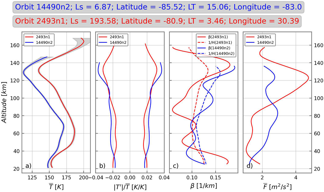
Figure 4. Vertical profiles of the calculated quantities corresponding to the “cold” (blue) and “warm” (red) ambient temperature: (a) Observed mean temperature $\bar{T}$; (b) amplitudes of relative wave temperature disturbances $|T^{\prime }|/\bar{T}$; (c) vertical damping rates $\beta$ (solid) and growth rates $1/H$ (dashed lines); (d) vertical flux of horizontal wave momentum $F$ (“wave momentum flux”).

Equation 4 provides insight into the vertical evolution of the wave momentum flux, which is determined by the balance of the growth and decay rates. These rates are plotted in Figure 4c with the dashed and solid lines, respectively. As can be seen, $F$ increases when $\beta <1/H$ and decreases when the opposite is true. The blue dashed lines for $1/H$ are always larger than the red ones, indicating that a colder atmosphere facilitates wave amplitude growth with altitude. This occurs because the atmosphere contracts at lower temperatures, enabling amplitude to exponentially grow over shorter vertical distances. Figure 4d illustrates this with the blue line representing the flux $F$ growing steeper than the red one up to $\sim$80 km. Convective instability and/or nonlinear breaking/saturation also tend to occur at larger amplitudes, which is illustrated by the rapid growth of $\beta$ above 70 km (blue line in panel c) and the resulting steep decline of $F$ (panel d). Equation 4, which describes the overall behavior of wave amplitudes and captures all these processes, also shows that growth and decay rates do not directly define the wave momentum flux $F$. Rather, their vertical integration is required. The complex nonlinear relationship between amplitudes and the damping rate $\beta$ partially explains the inconclusive and mixed results regarding the correlation between $F$ and mean temperature shown in the bottom row of Figure 2.

5 Conclusion

High-resolution ($\sim$4–5 km) vertical profiles of ${\text{CO}}_2$ density and temperature obtained from the ACS-TGO solar occultation measurements enabled the retrieval of gravity waves within a wide range of altitudes (between approximately 10 and 160 km) and to assess their vertical decay. The main conclusions of this research based on the dataset covering more than 6 years of observations from April 2018 to October 2024, that is 3.5 MYs, are as follows.

1. Relative temperature disturbances associated with GWs show some positive correlation with the Brunt-Väisälä frequency and an anticorrelation with the mean temperature near the mesopause only, where the mean lapse rate is small. However, no clear relationship was found at other altitudes. These results are consistent with the previous analyses based on different observations that found a correlation only at certain altitudes, and with the assertion that convective instability may play a role in the observed distributions of waves in the mesopause region.

2. The derived vertical profiles of the wave momentum flux $F$ agree well with the theoretical predictions (equation), according to which the vertical evolution of $F$ is determined by the balance between the growth and decay rates due to the density decrease and dissipation, respectively.

3. We found an unexpectedly persistent anticorrelation between the damping rates and the mean ambient temperature at all seasons and heights above $\sim$20 km. While it can be partially attributed to nonlinear saturation/breaking and dissipation due to molecular diffusion above $\sim$80 km, the reason for this behavior below 80 km remains unclear.

In closing, the latter anticorrelation occurs in all seasons (see Figure 4), i.e., with very different wind distributions. Therefore, it seems unlikely that critical-level filtering by seasonally varying winds alone explains the observed behavior. Further dedicated studies are required to explain this phenomenon.

Data availability statement

The ACS data are available from the ESA Planetary Science Archive (PSA; https://archives.esac.esa.int/psa/%23!Table%20View/ACS=instrument#!Home%20View). The temperature vertical profiles retrieved from ACS-NIR and ACS-MIR measurements are due to Fedorova et al. (2023) and Belyaev et al. (2022) respectively. The data supporting figures are also available at https://data.mendeley.com/datasets/ksjvg6vvx3/1.

Author contributions

ES: Conceptualization, Data curation, Formal Analysis, Investigation, Methodology, Writing – original draft, Writing – review and editing, Software. AM: Conceptualization, Methodology, Writing – original draft, Writing – review and editing. DB: Data curation, Funding acquisition, Investigation, Methodology, Resources, Supervision, Writing – original draft, Writing – review and editing. AF: Data curation, Investigation, Resources, Writing – review and editing. AT: Data curation, Project administration, Resources, Writing – review and editing. PH: Methodology, Writing – review and editing. FM: Project administration, Writing – review and editing. OK: Funding acquisition, Supervision, Writing – review and editing.

Funding

The author(s) declare that financial support was received for the research and/or publication of this article. Russian Science Foundation N. 25-22-00494.

Acknowledgments

ES and DB acknowledge support from the Russian Science Foundation (RSF N. 25-22-00494) for the retrievals of ACS-MIR vertical profiles and for all data analysis.

Conflict of interest

The authors declare that the research was conducted in the absence of any commercial or financial relationships that could be construed as a potential conflict of interest.

Generative AI statement

The author(s) declare that no Generative AI was used in the creation of this manuscript.

Any alternative text (alt text) provided alongside figures in this article has been generated by Frontiers with the support of artificial intelligence and reasonable efforts have been made to ensure accuracy, including review by the authors wherever possible. If you identify any issues, please contact us.

Publisher’s note

All claims expressed in this article are solely those of the authors and do not necessarily represent those of their affiliated organizations, or those of the publisher, the editors and the reviewers. Any product that may be evaluated in this article, or claim that may be made by its manufacturer, is not guaranteed or endorsed by the publisher.

References

Belyaev, D., Fedorova, A., Trokhimovskiy, A., Alday, J., Montmessin, F., Korablev, O., et al. (2021). Revealing a high water abundance in the upper mesosphere of Mars with ACS onboard TGO. Geophys. Res. Lett. 48, e2021GL093411. doi:10.1029/2021GL093411

CrossRef Full Text | Google Scholar

Belyaev, D., Fedorova, A., Trokhimovskiy, A., Alday, J., Montmessin, F., Korablev, O., et al. (2022). Thermal structure of the middle and upper atmosphere of Mars from ACS/TGO CO₂ spectroscopy. J. Geophys. Res. Planets 127, e2022JE007286. doi:10.1029/2022JE007286

CrossRef Full Text | Google Scholar

England, S. L., Liu, G., Yiğit, E., Mahaffy, P. R., Elrod, M., Benna, M., et al. (2017). MAVEN NGIMS observations of atmospheric gravity waves in the martian thermosphere. J. Geophys. Res. Space Phys. 122, 2310–2335. doi:10.1002/2016JA023475

CrossRef Full Text | Google Scholar

Ern, M., Preusse, P., Alexander, M. J., and Warner, C. D. (2004). Absolute values of gravity wave momentum flux derived from satellite data. J. Geophys. Res. Atmos. 109, D20103. doi:10.1029/2004JD004752

CrossRef Full Text | Google Scholar

Fedorova, A., Montmessin, F., Korablev, O., Luginin, M., Trokhimovskiy, A., Belyaev, D., et al. (2020). Stormy water on Mars: the distribution and saturation of atmospheric water during the dusty season. Science 367, 297–300. doi:10.1126/science.aay9522

PubMed Abstract | CrossRef Full Text | Google Scholar

Fedorova, A., Montmessin, F., Trokhimovskiy, A., Luginin, M., Korablev, O., Alday, J., et al. (2023). A two-martian years survey of the water vapor saturation state on Mars based on ACS NIR/TGO occultations. J. Geophys. Res. Planets 128, e2022JE007348. doi:10.1029/2022JE007348

CrossRef Full Text | Google Scholar

Fritts, D. C., Tsuda, T., Kato, S., Sato, T., and Fukao, S. (1988). Observational evidence of a saturated gravity wave spectrum in the troposphere and lower stratosphere. J. Atmos. Sci. 45, 1741–1759. doi:10.1175/1520-0469(1988)045-1741:OEOASG-2.0.CO;2

CrossRef Full Text | Google Scholar

Jesch, D., Medvedev, A. S., Castellini, F., Yiğit, E., and Hartogh, P. (2019). Density fluctuations in the lower thermosphere of Mars retrieved from the ExoMars trace gas orbiter (TGO) aerobraking. Atmosphere 10, 620. doi:10.3390/atmos10100620

CrossRef Full Text | Google Scholar

Korablev, O., Montmessin, F., Trokhimovskiy, A., Fedorova, A., Shakun, A., Grigoriev, A., et al. (2018). The atmospheric chemistry suite (ACS) of three spectrometers for the ExoMars 2016 trace gas orbiter. Space Sci. Rev. 214, 7. doi:10.1007/s11214-017-0437-6

CrossRef Full Text | Google Scholar

Kuroda, T., Yiğit, E., and Medvedev, A. S. (2019). Annual cycle of gravity wave activity derived from a high-resolution Martian general circulation model. J. Geophys. Res. Planets 124, 1618–1632. doi:10.1029/2018JE005847

CrossRef Full Text | Google Scholar

Kuroda, T., Medvedev, A. S., and Yiğit, E. (2020). Gravity wave activity in the atmosphere of Mars during the 2018 global dust storm: simulations with a high-resolution model. J. Geophys. Res. Planets 125, e2020JE006556. doi:10.1029/2020JE006556

CrossRef Full Text | Google Scholar

Leelavathi, V., Venkateswara Rao, N., and Rao, S. V. B. (2020). Interannual variability of atmospheric gravity waves in the martian thermosphere: effects of the 2018 planet-encircling dust event. J. Geophys. Res. Planets 125, e2020JE006649. doi:10.1029/2020JE006649

CrossRef Full Text | Google Scholar

Liu, J., Millour, E., Forget, F., Gilli, G., Lott, F., Bardet, D., et al. (2023). A surface to exosphere non-orographic gravity wave parameterization for the Mars planetary climate model. J. Geophys. Res. Planets 128, e2023JE007769. doi:10.1029/2023JE007769

CrossRef Full Text | Google Scholar

Medvedev, A. S., and Klaassen, G. P. (2000). Parameterization of gravity wave momentum deposition based on nonlinear wave interactions: basic formulation and sensitivity tests. JASTP 62, 1015–1033. doi:10.1016/S1364-6826(00)00067-5

CrossRef Full Text | Google Scholar

Medvedev, A. S., and Yiğit, E. (2019). Gravity waves in planetary atmospheres: their effects and parameterization in global circulation models. Atmosphere 10, 531. doi:10.3390/atmos10090531

CrossRef Full Text | Google Scholar

Nakagawa, H., Terada, N., Jain, S. K., Schneider, N. M., Montmessin, F., Yelle, R. V., et al. (2020). Vertical propagation of wave perturbations in the middle atmosphere on Mars by MAVEN/IUVS. J. Geophys. Res. Planets 125, e2020JE006481. doi:10.1029/2020JE006481

CrossRef Full Text | Google Scholar

Shaposhnikov, D. S., Medvedev, A. S., Rodin, A. V., Yiğit, E., and Hartogh, P. (2022). Martian dust storms and gravity waves: disentangling water transport to the upper atmosphere. J. Geophys. Res. Planets 127, e2021JE007102. doi:10.1029/2021JE007102

CrossRef Full Text | Google Scholar

Siddle, A., Mueller-Wodarg, I., Stone, S., and Yelle, R. (2019). Global characteristics of gravity waves in the upper atmosphere of Mars as measured by MAVEN/NGIMS. Icarus 333, 12–21. doi:10.1016/j.icarus.2019.05.021

CrossRef Full Text | Google Scholar

Starichenko, E. D., Belyaev, D. A., Medvedev, A. S., Fedorova, A. A., Korablev, O. I., Trokhimovskiy, A., et al. (2021). Gravity wave activity in the Martian atmosphere at altitudes 20–160 km from ACS/TGO occultation measurements. J. Geophys. Res. Planets 126, e2021JE006899. doi:10.1029/2021JE006899

CrossRef Full Text | Google Scholar

Starichenko, E. D., Medvedev, A. S., Belyaev, D. A., Yiğit, E., Fedorova, A. A., Korablev, O. I., et al. (2024). Climatology of gravity wave activity based on two martian years from ACS/TGO observations. Astron. Astrophys. 683, A206. doi:10.1051/0004-6361/202348685

CrossRef Full Text | Google Scholar

Terada, N., Leblanc, F., Nakagawa, H., Medvedev, A. S., Yiğit, E., Kuroda, T., et al. (2017). Global distribution and parameter dependences of gravity wave activity in the Martian upper thermosphere derived from MAVEN/NGIMS observations. J. Geophys. Res. Space Phys. 122, 2374–2397. doi:10.1002/2016JA023476

CrossRef Full Text | Google Scholar

Vals, M., Spiga, A., Forget, F., Millour, E., Montabone, L., and Lott, F. (2019). Study of gravity waves distribution and propagation in the thermosphere of Mars based on MGS, ODY, MRO and MAVEN density measurements. Planet. Space Sci. 178, 104708. doi:10.1016/j.pss.2019.104708

CrossRef Full Text | Google Scholar

Yiğit, E., and Medvedev, A. S. (2010). Internal gravity waves in the thermosphere during low and high solar activity: simulation study. J. Geophys. Res. Space Phys. 115. doi:10.1029/2009JA015106

CrossRef Full Text | Google Scholar

Yiğit, E., and Medvedev, A. S. (2019). Obscure waves in planetary atmospheres. Phys. Today 6, 40–46. doi:10.1063/PT.3.4226

CrossRef Full Text | Google Scholar

Yiğit, E., England, S. L., Liu, G., Medvedev, A. S., Mahaffy, P. R., Kuroda, T., et al. (2015). High-altitude gravity waves in the martian thermosphere observed by MAVEN/NGIMS and modeled by a gravity wave scheme. Geophys. Res. Lett. 42, 8993–9000. doi:10.1002/2015GL065307

CrossRef Full Text | Google Scholar

Yiğit, E., Medvedev, A. S., Benna, M., and Jakosky, B. M. (2021a). Dust storm-enhanced gravity wave activity in the martian thermosphere observed by MAVEN and implication for atmospheric escape. Geophys. Res. Lett. 48, e2020GL092095. doi:10.1029/2020GL092095

CrossRef Full Text | Google Scholar

Yiğit, E., Medvedev, A. S., and Hartogh, P. (2021b). Variations of the Martian thermospheric gravity-wave activity during the recent solar minimum as observed by MAVEN. Astrophysical J. 920, 69. doi:10.3847/1538-4357/ac15fc

CrossRef Full Text | Google Scholar