Estimation and assessment of solar wind propagation time from the Lagrange point L1 to Earth’s bow shock

The solar wind (SW) passing the Earth is an important driver of electrodynamic processes in the Earth’s magnetosphere–ionosphere–thermosphere (MIT) system. Since SW observations near Earth (at the bow shock) are very sparse, research and operational applications typically rely on measurements of SW monitors at the Lagrange point L1. The data of these monitors, which provide almost continuous datasets, need to be propagated in time to the bow shock conditions in order to be most useful for MIT studies. The most widely used data source for propagated SW data is provided by OMNIWeb. Near-Earth (NE) SW observations are highly relevant for the validation of the propagated SW estimates. This work uses the NE SW observations to propose a novel method for the estimation of the SW propagation delay. It is based on careful data assessment and a complex combination of correlation analysis and validation metrics. The developed algorithm generates a large dataset of 53,880 events in the period from 22 December 2017 to 30 April 2024, which provides the SW delay along with a list of metrics indicating the quality of the match between the SW structures at L1 and the bow shock. This dataset shows higher reliability in the SW delay estimates than the OMNIWeb data because it focuses on the comparison of structures in the SW. Using the dataset of the period from December 2017 to February 2018, the statistically estimated delay in comparison with the OMNIWeb data reveals that approximately $50\%$ of the delays are computed very accurately with less than 5 min uncertainty, and $80\%$ of the OMNIWeb data delay is reasonably accurate with less than 10 min difference from the statistically estimated delay, providing the best match. However, more than $5\%$ of the OMNIWeb data shows large differences of more than 20 min from the dataset. Thus, it can be concluded that in many cases, the uncertainty in the OMNIWeb delay estimate is larger than the value provided with the data. The generated dataset of SW delay estimates provides an ideal foundation for validating and improving solar wind propagation models.

1 Introduction

The solar wind (SW) and embedded interplanetary magnetic field (IMF) play significant roles in Earth’s magnetosphere and ionosphere system dynamics and control the space weather and its impacts on technological systems. The influence of space weather on the performance and reliability of the increasingly sophisticated ground-based and in situ technological system dramatically raises our vulnerability to space weather events. Accurate predictions of the near-Earth (NE) SW and IMF are essential to correctly describe the space weather operation and address the cause of magnetospheric phenomena and dynamics. In addition, the SW and IMF parameters are used as inputs in many magnetospheric and ionospheric models (Roble and Ridley, 1994; Lotz et al., 2017; Ferreira et al., 2020). The solar wind and magnetic field parameters are often provided by the Advanced Composition Explorer (ACE) and WIND spacecraft and more recently by Deep Space Climate Observatory (DSCOVR), all of which orbit around the first Lagrange point (L1).

The spacecraft measurements at the L1 point, however, must be converted to Earth’s bow shock before usage for research or operation purposes. Because of the large distance ($\sim 230$ Earth radii $R_E$) of the L1 point from Earth and because the spacecraft can be up to 100 $R_E$ off the Earth–Sun line, the transformation has not always been accurate, and this potentially decreases the quality of space weather forecasts. The knowledge of SW propagation time from L1 monitors to Earth’s bow shock helps us broaden our understanding of how the geospace system responds to the ever-changing SW, and it provides an advanced prediction of the approaching SW features. An accurate prediction of the ionospheric and thermospheric conditions depends on how accurate the predictions of the arrival time of the SW and severe solar wind conditions at Earth’s magnetosphere are, in addition to other factors. The forecast of the onset time of geomagnetic disturbances also depends on the accuracy of the predicted SW delay. Solar wind plasma and IMF parameters at the Earth’s bow shock location, as predicted by OMNIWeb (Lethy et al., 2018) and derived using the flat plane method (Wintoft et al., 2017), are frequently utilized in models for predicting and forecasting the disturbance storm time (DST) index and planetary $K_p$ index. A wrong estimation will result in an incorrect prediction.

In addition, the information on SW delay/offset is valuable for users of communication and navigation services who seek timely and reliable data to anticipate potential service malfunctions or outages. SW propagation delay is often referred to as SW delay, offset, time-shift, and lag. The SW propagation delay or SW delay refers to the time it takes for the solar wind to travel from the L1 point to the Earth. In other words, the SW observed at Earth is delayed relative to that observed at L1 due to the finite propagation time needed by the SW to travel from L1 to Earth. Several investigations have focused on modeling the time delay of solar wind propagation from spacecraft at L1 to Earth to address the above points, and numerous studies, including Ridley (2000), Wu et al. (2005), Mailyan et al. (2008), Pulkkinen and Rastätter (2009), Haaland et al. (2010), Cash et al. (2016), Baumann and McCloskey (2021), and Cameron and Jackel (2016), have contributed to this field. Additionally, research areas such as the timing of polar substorm onset, as explored by Baker et al. (2002) and Lyons and Nishimura (2020), can also benefit from precise information regarding the arrival of solar wind features that may trigger such events in the magnetosphere.

The earlier studies (Mailyan et al., 2008; Cash et al., 2016) suggested that the propagation time is often on the order of 1 h, and the specific value depends closely on the SW conditions. Various methods (Mailyan et al., 2008; Case and Wild, 2012; Cash et al., 2016) have been proposed to calculate the exact propagation time based on the observed SW conditions around L1. The simplest one computes the time by dividing the distance in the geocentric solar ecliptic (GSE) X direction by the SW velocity (Collier et al., 1998). This method is called “flat delay” or “ballistic propagation” and is currently used by NOAA’s Space Weather Forecast Office (Cash et al., 2016). The flat delay method assumes simply a planar propagation (in the $X$ direction only) in the anti-sunward direction where the solar wind travels from any selected point (e.g., L1 point) to another point (e.g., Earth bow shock location) without any fundamental changes in the solar wind properties. The NOAA Space Weather Forecast Office is currently using this technique to predict the solar wind propagation delay. The solar wind flat delay (Case and Wild, 2012; Cash et al., 2016; Baumann and McCloskey, 2021), therefore, is calculated using the following expression:

$\mathrm{\Delta }{t}_{ft}=\frac{\mathrm{\Delta }{S}_X}{\overline{V_X}}.(1)$

The flat plane method enables calculation of the solar wind delay when SW speed data are available at the L1 location. However, this method is limited by insufficient information and the influence of the orientation of the SW phase planes on propagation delay (Ridley, 2000; Horbury et al., 2001; Weimer et al., 2003; Weimer, 2004; Baumann and McCloskey, 2021). Phase planes refer to structures in the SW that are usually contained in planar structures, and the orientation of these planes, called the phase front normal (PFN), can be tilted at arbitrary angles with respect to the Sun–Earth line. When the PFN is tilted, an L1 monitor displaced from the Sun–Earth line will observe an IMF structure at a different time than if it were located on the Sun–Earth line (Mailyan et al., 2008). A realistic calculation of propagation time should, therefore, consider PFN.

Determining the PFN, however, is a complex task, and a suite of methods has been developed. Two widely used approaches are minimum variance analysis (MVA) (Weimer et al., 2003; Weimer, 2004; Bargatze et al., 2005; Weimer and King, 2008; Pulkkinen et al., 2011; Haaland et al., 2006; Munteanu et al., 2013) and cross product (CP) method (Horbury et al., 2001; Knetter et al., 2004). The former defines the PFN as the minimum variance direction of the IMF with an additional constraint that the average magnetic field along the PFN should be zero. The latter specifies the PFN as the direction of the cross-product of two averaged magnetic field vectors located upstream and downstream of the phase front. The difficulty in accurately predicting the propagation time was the primary reason for developing OMNIWeb, where a combination of MVA and CP methods is used to routinely lag the IMF and SW parameters from L1 to Earth’s bow shock.

OMNIWeb’s website (http://omniweb.gsfc.nasa.gov/) provides 1-min and 5-min high-resolution (HR) compiled records of ACE, IMP-8, GEOTAIL, and WIND spacecraft observations. The OMNIWeb database is the primary source of the SW data for the space weather research, where the datasets are time-shifted from the spacecraft (ACE, IMP-8, GEOTAIL, or WIND) position to the nose of the Earth bow shock. The expression for the solar wind time-shift used by OMNIWeb is

$\mathrm{\Delta }{t}_{\mathit{OMNI}}=\frac{\mathbf{n}\cdot \left({\mathbf{R}}_{\mathbf{B}}-{\mathbf{R}}_{\mathbf{O}}\right)}{\mathbf{n}\cdot \mathbf{V}},(2)$

where $\mathbf{V}$ presents the solar wind velocity, ${\mathbf{R}}_{\mathbf{O}}$ is the location of the observer (location of the spacecraft at the L1 point), the location of the Earth bow shock is ${\mathbf{R}}_{\mathbf{B}}$, $\cdot$ represents the scalar product of two vectors, and $\mathbf{n}$ is the variation PFN. The Earth’s bow shock location is determined using the bow shock model of Farris and Russel (2017) and the magnetopause model of Shue et al. (1997).

Significant efforts have been made to optimize the parameterization of MVA and CP methods by calibrating against the multiple spacecraft (ACE, WIND, IMP-8, and GEOTAIL) technique (Weimer et al., 2003; Weimer, 2004; Weimer and King, 2008; Munteanu et al., 2013). This technique determines the propagation time as time-shifts that produce the best match-up of IMF structures observed by different spacecraft. Despite the efforts, the existing parameterization still generates estimations that are considerably different from the actual values. The statistical study of Mailyan et al. (2008) calculated the propagation delay of IMF discontinuities between the ACE solar wind motor at L1 and the Cluster quartet of spacecraft close to the Earth’s bow shock and found that the difference was $\ge 5$ min for $\ge 30\%$ of the time. Both Mailyan et al. (2008) and Cash et al. (2016) detected situations where the difference becomes $\ge 30$ min. The OMNIWeb assumes that the parameters do not evolve over space and in time, but the actual SW is not homogeneous. Evidence has shown that variability exists in the SW perpendicular to the Sun–Earth line, that phase fronts may not be planar on large scales, and moreover, that the SW evolves during propagation (Tsurutani et al., 2005; Borovsky, 2010). Inaccurate SW specifications provided by OMNIWeb have been reported to have high costs in modeling specific events (Ashour-Abdalla et al., 2008; Fredrick et al., 2025).

The present study aims to develop an improved statistical algorithm to address the SW propagation delay problem in space weather prediction. The algorithm will be used to generate a large dataset of estimated SW delays and corresponding magnetic field components and SW parameters using multiple spacecraft pairs at L1 and near-Earth locations. The algorithm focuses on matching SW features around the L1 point (ACE, DSCOVR, and WIND) and upstream of the bow shock (MMS, CLUSTER, and GEOTAIL) by computing the variance and cross-correlation coefficient. In addition, a qualitative and quantitative comparison to OMNIWeb data and other delay models will be applied to estimate and discuss the uncertainties of the different approaches. Finally, factors limiting the accuracy of our delay estimations and the OMNIWeb-provided delay will be assessed and discussed. The estimated delay and associated datasets will allow us to test and validate existing SW propagation delay predictions, develop improved prediction models, and use them for further SW predictions. The manuscript is structured as follows: Section 2 describes the data sources and preprocessing. Section 3 introduces the methods, estimation techniques, and the database of the solar wind propagation delay used in this study. Section 4 provides a description of the generated dataset based on some examples for different spacecraft pairs. Section 5 compares the estimated delay with the results of existing methods. Section 6 discusses the results. In Section 7, we present the conclusions.

2 Data source and preprocessing

To obtain the SW and IMF parameters around L1, we use ACE, DSCOVR, and WIND spacecraft. Magnetospheric Multiscale (MMS), CLUSTER, and GEOTAIL data are employed for parameters upstream of Earth’s bow shock. The available dataset spans over two decades using multiple combinations of spacecraft pairs, one at L1 and the other being near-Earth, from 1997 to the present. An example of the spacecraft orbits is plotted for the period from 1 July 2017 to 1 March 2018 in Figure 1. Table 1 lists the launch year, orbit, and the instruments of each spacecraft utilized in this investigation. For the current study, the spacecraft pairs and observations of the selected data period in Table 2 were chosen for convenience.

Figure 1

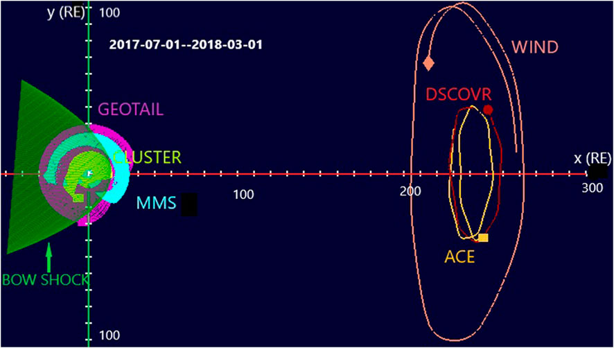
Figure 1. Orbits of ACE, WIND, DSCOVR, GEOTAIL, CLUSTER, and MMS 1 in GSE coordinates during 1 July 2017 and 1 March 2018, using NASA’s 4D Orbit Viewer. The green parabola illustrates Earth’s bow shock.

Table 1

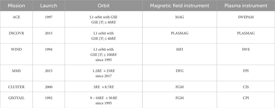
Table 1. Launch year, orbit, and instruments utilized by various spacecraft.

Table 2

Table 2. Spacecraft pairs and corresponding data period used in the current analyses.

We focus on periods where one spacecraft is located around the L1 point and another is upstream of the bow shock. Over the selected data interval in Table 2, we apply the following criteria on the NE monitors’ data (MMS, CLUSTER, and GEOTAIL):

1. The NE monitors are located at $X>14$ RE and $|Y|<15$ RE (Mailyan et al., 2008; Cash et al., 2016) to have a good chance of having the spacecraft at the bow shock, i.e., to obtain solar wind observations upstream of the bow shock.

2. The ion temperature for the selected interval requires to have a value $<1\mathrm{k}\mathrm{e}\mathrm{V}$ (Mailyan et al., 2008) to avoid bow-shock and fore-shock activities.

3. The magnetic field variance for the data window (a window consists of five consecutive data points or time series data over 75 s) needs to be below a threshold to exclude Earth foreshock events and high-fluctuation magnetic field components. We calculate the variance over each set of five data points in a data window and exclude any window where the variance exceeds 50 nT.

Because different instruments and different spacecraft provide data at different cadences, we resample all the data to one common cadence. The new cadence should be sufficiently high for capturing sharp variations in the SW. Following the high-resolution OMNIWeb (HRO) dataset, which utilizes WIND magnetic field data at 15-s resolution and ACE at 16-s resolution, we resample the data to a cadence of 15 s, where the data are first averaged with a 15-s sliding window and then interpolated at a 15-s resolution. Similarly, we resample MMS, DSCOVR, CLUSTER, and GEOTAIL spacecraft data to 15 s for this study. We interpolate the observations of magnetic field components and the SW parameters only if the data gap is <1 minute.

3 Methodology

3.1 Correlating IMF at L1 and near-Earth and obtaining propagation times

Performing a correlation analysis on time series data observed at the L1 point and the equivalent time series measured close to the Earth allows us to calculate the offset or the time delay. However, choosing an appropriate correlation method for a problem is not straightforward; instead, it can be problem- and data-specific. Cross-correlation (Case and Wild, 2012) and Pearson linear correlation (Vokhmyanin et al., 2019) are two methods that were applied before to solve solar wind propagation delay prediction and estimation. Therefore, we start by comparing the cross-correlation and Pearson linear correlation to select the better correlation coefficient (CC) approach for our problem. We first employ the Pearson linear CC, following the Vokhmyanin et al. (2019) approach. Vokhmyanin et al. (2019) employed the generalized Pearson linear correlation for the magnetic field vector as follows:

$C{C}_{B_{y,z}}=\frac{{\sum }_{i=1}^{N}d{B}_{\mathit{Liy}}d{B}_{\mathit{NEiy}}+d{B}_{\mathit{Liz}}d{B}_{\mathit{NEiz}}}{\sqrt{{\sum }_{i=1}^N\left[d{B}_{\mathit{Liy}}^2+d{B}_{\mathit{Liz}}^2\right]}\sqrt{{\sum }_{i=1}^N\left[d{B}_{\mathit{NEiy}}^2+d{B}_{\mathit{NEiz}}^2\right]}},(3)$

where $L$ represents the spacecraft at the L1 point and $NE$ presents spacecraft at the near-Earth location. $y$ and $z$ denote two components of the magnetic field in GSE coordinates, $i$ is the number of data points within a 20-min sliding window, and $d{B}_i$-s show the deviations from the mean value (mean of 20 min data window) of each component of the IMF vector. Here, the resolution of the data is 15 s. Therefore, we have $N=80$ data points in each 20-min window.

We perform cross-correlation analysis between data around L1 and near-Earth on the parameter IMF clock angle, which is defined as

$\theta =\arctan \frac{B_y}{B_z},(4)$

in GSE coordinates. As noted by Case and Wild (2012), the clock angle (Equation 4) serves as an ideal parameter for tracing SW because it provides an overview measure of the IMF rather than a singular component of the IMF. Moreover, the use of the cross-correlation method provides a slightly better number of estimated delays than that when using the field magnitude. The cross-correlation $CC$ of the populations ${\theta }_{NE}$ and ${\theta }_{L1}$ as a function of the lag (L) is

$C{C}_{{\theta }_{NE},{\theta }_{L1}}\left(L\right)=\frac{{\sum }_{i=1}^{N-|L|}\left({\theta }_{NE,i+|L|}-\langle {\theta }_{NE}\rangle \right)\left({\theta }_{L1,i}-\langle {\theta }_{L1}\rangle \right)}{\sqrt{{\sum }_{i=1}^N{\left({\theta }_{NE,i}-\langle {\theta }_{NE}\rangle \right)}^2{\sum }_{i=1}^N{\left({\theta }_{L1,i}-\langle {\theta }_{L1}\rangle \right)}^2}},(5)$

where $⟨\theta ⟩$ is the average of the calculated clock angle and $L1$ and $NE$ represent the L1 point and near-Earth locations.

Pearson correlation is performed between the components of the magnetic fields of $L1$ (ACE) and near-Earth (MMS) monitors, while cross-correlation is performed between the clock angles of the respective spacecraft. We calculate the $C{C}_{B_{y,z}}$ for only $B_y$ and $B_z$ to make a fair comparison with $C{C}_{{\theta }_{NE},{\theta }_{L1}}$ as the clock angle only considers $B_y$ and $B_z$.

The procedure for the calculation of the lag time is as follows: We take 20 min of L1 data and 2 h of NE data, starting at exactly the same time as the L1 data. We apply a 20-min moving window, shifting in 1-min steps along the 2 h of NE data. For each shift along the 2 h of NE data, we compute the correlation coefficients between the 20 min of NE data and the 20 min of L1 data, as described above. Then, we assess the correlation coefficients for its maxima. If the coefficients $(CC)$ within these segments only show one single peak, or if they show multiple peaks but one peak dominates the others (>200% higher than the others), the offset (considering the shifted time of the sliding window) corresponding to this peak is determined as the SW propagation time.

After the identification of the shift or offset with the maximum $CC$, the $CC$ conditions are assessed with respect to the quality conditions and outliers as described in Subsections 3.2, 3.3 to identify if it is a “good case.” We use the term “good cases” for the selected estimated delay values where all three criteria in Section 2 are fulfilled and all quality conditions pointed out in Section 3.2 are satisfied. All the good cases are included in our datasets and presented in Section 4. This concludes the analysis of this 20-minute L1 data, and the procedure is repeated for the next 20-min L1 data window by sliding by 5 min at a time, which overlaps with the previous for 15 min.

To select cases with high correlation coefficients, we set a requirement that $CC$ values must be positive and at the maximum peak $CC\ge 0.5$. Figure 2 [panel (a)] shows the number of good cases versus the estimated delay for the period from December 2017 to March 2018 using clock angle $C{C}_{{\theta }_{NE},{\theta }_{L1}}$ and magnetic field component $C{C}_{B_{y,z}}$ methods. The upper bound of the estimated delay is considered 100 min since very slow solar wind (with a speed of 300 ${\mathrm{k}\mathrm{m}\mathrm{s}}^{-1}$) reaches Earth in 90 min (Baumann and McCloskey, 2021). The lower bound is considered 20 min since extremely fast SW (with a speed of 1,000 ${\mathrm{k}\mathrm{m}\mathrm{s}}^{-1}$) reaches Earth in 20 min (Baumann and McCloskey, 2021). The delay values $>100$ minutes or <20 minutes are considered out-of-range data points, which are excluded in Figure 2.

Figure 2

Figure 2. [Panel (a)] Distributions of the statistically estimated delay employing correlation coefficient $C{C}_{B_{y,z}}$ using magnetic field components (Equation 3) and correlation coefficient using clock angle $C{C}_{{\theta }_{NE},{\theta }_{L1}}$ (Equation 5). Here, blue and green bars show the number of good cases for $C{C}_{B_{y,z}}$ and $C{C}_{{\theta }_{NE},{\theta }_{L1}}$, respectively. If all three criteria in Section 2 are met and all required conditions of Section 3.2 are satisfied, we define the estimated results as good cases. The horizontal scale is limited to 20 min–100 min. Few cases for both $C{C}_{B_{y,z}}$ and $C{C}_{{\theta }_{NE},{\theta }_{L1}}$ are out of this scale. [Panel (b)] Profiles of the statistical indices and CC coefficients. Here, correlation analyses are performed between the observations of ACE and MMS for the period from December 2017 to March 2018.

The histogram excludes the out-of-range values and shows that the $C{C}_{\theta }$ method provides higher correlation values than that of $C{C}_{B_{y,z}}$. Since we aim to apply our statistical algorithm to estimate solar wind propagation delay as continuously as possible, the number of good cases is significant in this analysis. Since the correlation analysis using the clock angle $C{C}_{{\theta }_{NE},{\theta }_{L1}}$ provides more good cases than that using magnetic field components $C{C}_{B_{y,z}}$, the cross-correlation $(CC)$ using the clock angle method is only employed for further analysis. An example of the cross-correlation profile (green line) of a good case for the period 00:00 UT to 01:40 UT on 13 December 2017 is depicted in Figure 2 [Panel (b)]. The red line depicts the plateau-shaped magnitude index (PMI), the black broken line shows the weighted correlation coefficient (weighted CC), the purple line shows the magnitude index (MI), the cyan line represents prediction efficiency (PE), the lime-green line depicts the non-dimensional measure of average error (NDME), and the blue line represents refined prediction efficiency (RPE). We explain the statistical indices PMI, weighted CC MI, PE, NDME, and RPE in the following section (Section 3.2).

3.2 Quality measurement and evaluation of correlation analysis

The magnitude of the CC is not sufficient to identify the physical correlation of two datasets. Therefore, we assessed a number of parameters that help provide sufficient confidence that the L1 and NE data with the detected offset/shift are correlated. We tested the following list of statistical parameters to assess $C{C}_{{\theta }_{NE},{\theta }_{L1}}$ (equivalent equations appropriate to magnetic field components are used to assess $C{C}_{B_{y,z}}$) on a period of 6 months of the ACE–MMS dataset (December 2017 to March 2018) to assess their applicability as a quality measure for the given problem:

1. Prediction efficiency (PE): A high correlation between two data series does not always present an identical data series (Vokhmyanin et al., 2019). Instead, it shows similarities in their variances. The correlation analysis fails when the variance of data becomes weaker than the noise in the data. To resolve this issue, it is important to find a suitable statistical parameter/index that is most appropriate for our problem. In search of an appropriate index, we first start with the PE matrix, which was used in the earlier analyses of Pulkkinen et al. (2011) and Vokhmyanin et al. (2019).

$PE=1-\frac{{\sum }_{i=1}^N{\left({\theta }_{NE,i}-{\theta }_{L1,i}\right)}^2}{{\sum }_{i=1}^N{\left({\theta }_{L1,i}-⟨{\theta }_{L1}⟩\right)}^2}.(6)$

The optimal value of $PE$ (Equation 6) is 1, which represents the perfect match between two datasets. $PE=0$ indicates that only the mean values of two datasets overlap, while negative $PE$ suggests that the difference between the two datasets exceeds the variance. However, the PE matrix approaches the optimal value and reduces to 0 relatively fast, which reduces the probability of good cases. Figure 2 [panel (b)] displays statistical indices for the period 00:00 UT to 01:40 UT on 13 December 2017, where the cyan line presents PE, and its value decreases to 0 relatively quickly.

1. Refined prediction efficiency (RPE): To avoid the reduction in the number of good cases, we use the RPE matrix (Willmott et al., 2012). RPE values approach the optimal value 1 more slowly than PE (Vokhmyanin et al., 2019; Pulkkinen et al., 2011), which is shown by the blue line in Figure 2 [panel (b)]. The RPE has a finite upper and lower bound.

$RPE=1-\frac{{\sum }_{i=1}^N|{\theta }_{NE,i}-{\theta }_{L1,i}|}{2{\sum }_{i=1}^N|{\theta }_{L1,i}-⟨{\theta }_{L1,i}⟩|},(7)$

when

${\displaystyle \sum _{i=1}^N}|{\theta }_{NE,i}-{\theta }_{L1,i}|\le 2{\displaystyle \sum _{i=1}^N}|{\theta }_{L1,i}-⟨{\theta }_{L1,i}⟩|.(8)$

Otherwise,

$RPE=\frac{2{\sum }_{i=1}^N|{\theta }_{L1,i}-⟨{\theta }_{L1,i}⟩|}{{\sum }_{i=1}^N|{\theta }_{NE,i}-{\theta }_{L1,i}|}-1.(9)$

The matrix RPE (Equations 7–9) can be interpreted in terms of the mean absolute error (MAE) and the mean absolute deviation.

1. Non-dimensional measure of average error (NDME): To evaluate the performance of RPE in response to varying patterns of differences between the time series data of ${\theta }_{NE}$ and ${\theta }_{L1}$, we employ Watterson’s index (Watterson, 1996; Willmott et al., 2012), which is named here as the dimensionless measure of average error. For convenience, we use the acronym NDME for the dimensionless measures of average error.

$NDME=\frac{2}{\pi }\arcsin \left[1-\frac{MSE}{{\sigma }_{{\theta }_{NE}}^2+{\sigma }_{{\theta }_{L1}}^2+{\left(\langle {\theta }_{NE,i}\rangle -\langle {\theta }_{L1,i}\rangle \right)}^2}\right],(10)$

where $MSE={(RMSE)}^2=\frac{1}{n}\ast \sum {({\theta }_{NE,i}-{\theta }_{L1,i})}^2$ represents the mean squared error, ${\sigma }_{{\theta }_{L1}}=\sqrt{\frac{1}{n}\sum {\theta }_{L1,i}-{\bar{\theta }}_{L1}}$ denotes the standard deviation of ${\theta }_{L1}$, and ${\sigma }_{{\theta }_{NE}}=\sqrt{\frac{1}{n}\sum {\theta }_{NE,i}-{\bar{\theta }}_{NE}}$ denotes the standard deviation of ${\theta }_{NE}$. In this study, ${\bar{\theta }}_{NE}$ and ${\bar{\theta }}_{L1}$ are the mean values of ${\theta }_{NE,i}$ and ${\theta }_{L1,i}$, respectively, where $i=\mathrm{1,2,3},\dots ,n$, and $n$ is the total number of data points. The $NDME$ (Equation 10) index (lime-green dashed line in Figure 2 [panel (b)]) relates standard deviation and $RMSE$. Pontius et al. (2008) and Willmott et al. (2012) showed that $RMSE$ helps distinguish between differences due to the quantity and those due to the location in two datasets. We find that the maxima of peaks for $RPE$ and $NDME$ mostly coincide at the same time. Therefore, we choose only $NDME$ for further investigation in this paper.

1. Plateau-shaped magnitude index (PMI): To specify the similarities and dissimilarities between the magnitudes of the clock angle profiles, we employ the PMI with an optimal value of 1 in a plateau shape (Mineo and Ruggieri, 2005; G. P. Bhattacharjee and Mohan, 1963). When the difference between two profiles becomes large, the PMI index decreases rapidly (red line of Figure 2 [panel (b)]). It reaches $0.0$ when there is no good match.

$PMI=k_a\times \frac{2.22}{1-X_A^{2a}},(11)$

where $k_a=(a/\pi )\sin \pi /2a$, $X_A={(⟨{\theta }_{NE,i}⟩-{\theta }_{L1,i})}^2/{\sigma }_{{\theta }_{L1}}^2$, and the free parameter $a=2$.

1. Magnitude index (MI): We compared $PMI$ with another statistical index, MI, to check which index performs better for our analysis, where $MI={\exp }^{-{(⟨{\theta }_{NE}⟩-⟨{\theta }_{L1}⟩)}^2/(2{\sigma }_{{\theta }_{L1}}^2)}$ and is shown by the purple line in Figure 2 [panel (b)]. The profile of $MI$ shows a narrow optimal value and decreases more slowly than $PMI$, which makes the performance of $PMI$ (Equation 11) slightly better than that of $MI$, so we use only $PMI$ for the rest of the analysis.

2. Weighted CC: To simplify, we combine cross-correlation coefficient with plateau-shaped magnitude index PMI as

$\text{W}eightedCC=CC\times PMI.(12)$

The black dashed line in Figure 2 [panel (b)] depicts the $\text{W}eightedCC$ (Equation 12).

Finally, the results of the assessment of the above statistical parameters allowed us to combine two quality conditions, which are applied to each (dominant) peak in the CC that is detected by the procedure described in Subsection 3.1.

$\mathrm{W}\mathit{e}\mathit{i}\mathit{g}\mathit{h}\mathit{t}\mathit{e}\mathit{d}CC>0.5,\mathrm{a}\mathrm{n}\mathrm{d}NDME\ge 0.4.(13)$

The thresholds of selecting good cases $CC$ and $NDME$ (Equation 10) are explained in the Supplementary Figure S2. Only those events (pairs of 20-min data from L1 and NE spacecraft) that fulfill the above condition (Equation 13) are included in the dataset for the assessment of the solar wind L1-NE propagation time. We search for segments containing a weighted CC $>0.5$ for each correlation profile and NDME $\ge 0.4$. The time-shift/offset of the L1 observation, corresponding to the single peak or the dominant peak, determines the SW delay/propagation time/offset. The vertical dotted line in Figure 2 [panel (b)] indicates the offset or delay where condition 13 is satisfied.

3.3 Outlier interpretation and treatment

To generate a large dataset and prepare it for further analyses, outlier identification and detection are essential tasks. If the estimated delay in our investigation is substantially different from the neighboring estimated values, we identify that data point as an outlier. For the current analysis, we predict an outlier using the interquartile range (IQR) method; IQR is the middle $50\%$ of data in a histogram. A total of $25\%$ of the data is in the first quartile (Q1), before the IQR starts, and thus, it is smaller than the data in the IQR. A total of $25\%$ of the data is in the last quartile (Q4), and thus, it is larger than the data in the IQR. If any data point lies over 1.5 IQRs and below the first quartile (Q1) or above the third quartile (Q3) in a dataset, that data point is defined as an outlier. We separate the outlier data from the regular data and store them for further analyses. To check the reliability of the outliers, we visually inspected outlier datasets generated using MMS and ACE observations for 6 months (December 2017–May 2018) to define outlier conditions in our datasets. For this inspection, we check the time series of 2 hours of calculated clock angle $\theta$ and magnetic field components ($B_x$, $B_y$, and $B_z$) MMS data overplotted with 20 min of ACE data. The ACE data are shifted by the estimated delay. Since the estimations are based on matching the SW features, we tried to understand why the correlation method yielded a delay.

For the outlier cases where the algorithm is not successful in matching the time series data from two spacecraft, we interpolate them using the neighboring regular estimated delay from the estimated delay before and after the outlier. We only interpolate the data gap if the time difference between the time series data of the neighboring estimated delay is $\le 15$ minutes. We then measure the cross correlation between the calculated clock angle $\theta$ using MMS data with the $\theta$ using ACE data. The $\theta$ value calculated using ACE data is shifted by the interpolated delay. If the correlation coefficient is higher than 0.6, we include the estimated delay using interpolation in the dataset. Otherwise, we store the data point for visual inspection. For visual examination, we stored the time series plots of clock angle and magnetic field vectors for the outlier data points and then checked them carefully. During this process, we found that some data points may not be outliers; even though these data points are distant from the remaining data points in the sample, that point is not necessarily an outlier. In other words, we identified a couple of outlier data points that may not cause incorrect predictions of the solar wind propagation delay. We retain as many exceptional data points as possible during the visual examination. The remaining outliers are excluded from the dataset.

Some interesting outlier points that we found through the process are discussed below. Figure 3 shows three different cases of estimated delays with a large difference from the neighboring data points, and they are detected by the IQR method as outlier data points. The first set of outliers is detected at approximately 23:10 UT (observed time at ACE or L1 location). These outlier points are shown in Figure 3 panel (a) and are marked by a black circle. The corresponding clock angle profiles using MMS observation and time-shifted ACE are shown in panel (b). These data points are falsely identified as outlier points. We noted these data points as outlier cases (i), which may be due to the existence of shock-like structures. An example is shown in Figure 3 [panel (b)], where the outlier point corresponds to a shock-like structure in MMS and ACE data for the period 22:50 UT–1:30 UT on December 23. Although the existence of shock-like structures mostly helps match the SW features observed at two locations, it sometimes can lead to outbound results. Outlier case (i) creates ambiguities in the automated estimations. We keep as many points as possible by manually handling them. We manually inspected 3 months of data from the 4 years of data presented to establish the method, which is approximately $5\%$ of the total data. For the remaining data $(95\%)$, we used the automated approach. We developed the automated approach, which only includes “good cases.” Some points, however, are compromised due to automated running for longer periods. The automated run covers approximately $95\%$ of the data presented in the manuscript.

Figure 3

Figure 3. (Left) Statistically estimated raw/unprocessed delay using data from ACE-MMS spacecraft (a, c) and ACE-CLUSTER pairs (e). (Right) Time series data of clock angles (b, d, f) for three outlier conditions in the left panels.

Another outlier point can result when the correlation method does not find a definite feature to match. We indicate that issue as outlier case (ii): if there is no particular distinct structure to match or periodicity in the solar wind data, the algorithm tries to perform the best match of the magnitude. In some cases, the algorithm ends up predicting outbound delays. Even with a visual examination, it is sometimes difficult to identify the best match. To avoid such difficulties, we exclude them from our data. Three outbound data points at approximately 01:55 UT of 13 December 2017 (time observed at ACE) are circled in Figure 3 [panel (c)], which we identify as outlier case (ii). Figure 3 [panel (d)] depicts corresponding clock angle profiles using MMS and shifted ACE as an example near 01:55 UT ACE time, where we visually inspect that ACE data can match both at 2:50 UT (time observed at MMS) with a delay of $\sim 57$ minutes or at 3:20 UT (MMS time) with a delay $\sim 77$ minutes. However, the algorithm estimated $\sim 77$ minutes, which is one of the good matches but outbound from the neighboring data points (Figure 3 [panel (c)]). These three outlier points and similar data points are excluded from the final dataset.

One challenge in the data analysis process was handling highly fluctuating magnetic fields, particularly in observations from MMS or other near-Earth monitors. Sometimes, these fluctuations are not present in observations of ACE or other L1 point spacecraft. The correlation method often fails to correlate these profiles and generates an unreliable delay. It is also not possible to identify the best match of the two datasets (L1 and NE observations) through visual inspection. These data points are noted as outlier cases (iii): fluctuating magnetic field components often lead to an unreliable delay. The IQR outlier detection method sometimes identifies them as outbound points, but it occasionally fails. Specifically, when the fluctuation is present for a longer period, the IQR method cannot successfully identify it. Four data points are circled close to 09:40 UT (time observed at ACE) in panel (e) of Figure 3, where these points are examples of outlier case (iii). The clock angle profiles using CLUSTER and shifted ACE observations are shown in panel (f). The profiles match well at a glance, but it is hard to tell whether the delay is reliable due to the presence of the fluctuating magnetic field. To resolve this issue, we excluded or avoided these cases by including constraints on the variance of the fields to avoid the highly fluctuating magnetic field (criterion iii in Section 2).

The remaining outliers identified by the IQR method are considered regular outbound points where the correlation method is not very successful in estimating the delay. Our algorithm identifies simple outlier points successfully and removes them automatically from the dataset.

4 Description of the solar wind delay dataset based on some examples

The dataset presented in this work comprises 53,880 events, covering 7 years (22 December 2017–30 April 2024) of observations of the ACE–MMS spacecraft pair and 2 years (22 December 2017–31 December 2019) of the DSCOVR–MMS pair. An “event” refers to the good cases where we can successfully apply our method to match 20 min of L1 observations with the 20 min of NE monitor observations to estimate SW delay. The datasets contain the estimated delay with the respective solar wind parameters, e.g., $B_x$, $B_y$, $B_z$, $x$ component of the solar wind velocity in GSE coordinates $v_{x,GSE}$, ion temperature $T_i$ observed at the L1 point, and positions of both the $NE$ monitor and the L1 spacecraft. Details of the datasets are presented later in this section and are available on the EU Open Research Repository Zenodo (https://doi.org/10.5281/zenodo.14765909).

Figures 4–6 demonstrate the methodology with examples of estimated offset/estimated delays for multiple spacecraft pairs where all three criteria in Section 2 are satisfied and the quality conditions in Subsection 3.2 are met. Panels (a)–(d) of Figure 4 depict the results using the ACE and MMS spacecraft pair, and panels (e)–(h) present the results using ACE and CLUSTER. Estimations using DSCOVR–MMS [panels (a)–(c)] and WIND–GEOTAIL [panels (d)–(f)] pairs are shown in Figure 5. Figure 6 shows the cross-comparison of the estimations using multiple spacecraft pairs for the same data period. The time offset between L1 data and near-Earth observation is the SW propagation delay, also known as the time delay. We will refer to the offset as the time delay for the remainder of the manuscript.

Figure 4

Figure 4. (Left) Cross-correlation analysis for the statistically estimated delay, statistical indices, clock angle in degrees, and magnetic field components using data from the ACE–MMS spacecraft pair for 19:00 UT–23:00 UT on 30 December 2017. The right panels show a similar statistical analysis using ACE–CLUSTER pairs for 01:00 UT–04:00 UT on 6 March 2018. We use cross-correlation analysis (b,f) with weighted CC, PMI, and NDME indices for the quality measure that helps in obtaining the SW propagation delay (a,b) from the L1 point to upstream or at the Earth bow shock. The observed ACE clock angle (c,g) and magnetic field components (d, h) shifted at MMS (left) and CLUSTER’s location (right).

Figure 5

Figure 5. Statistically estimated delay (a, d), magnetic field components (b, e), and clock angle in degrees (c, f) using data from the DSCOVR–MMS spacecraft pairs for the period 18:00 UT–22:00 on 27 December 2017 (left) and similar analysis for the WIND–GEOTAIL pairs for 12:00 UT–17:00 UT on 16 December 2001 (right). The observed magnetic field components (b, e) and clock angle (c, f) data from DSCOVR (left) and WIND (right) shifted at MMS’s location (left) and GEOTAIL’s location (right). Here, we use linear interpolation to fill up the data gaps.

Figure 6

Figure 6. [Panel (a)] Cross-comparison of statistically estimated delay using data from the DSCOVR–MMS, ACE–CLUSTER, and ACE–MMS spacecraft pairs for the same period 08:00 UT–12:00 UT on 5 February 2018. Magnetic field (b) components at the t1 point for the three spacecraft pairs are depicted in panel (b) [ACE–CLUSTER], panel (c) [ACE–MMS], and panel (d) [DSCOVR–MMS], where each pair provides very similar results. Panels (e) and (f) show the B components for the t2 point, where DSCOVR–MMS provides a much higher delay ($\sim 10$ minutes larger) than the other two pairs.

Figure 4a shows the delay/offsets for the period 19:00 UT–23:00 UT on 30 December 2017 using ACE and MMS data. The color bar shows values of cross-correlation coefficient $(CC)$. For this example, we observe a high correlation between the clock angles calculated using ACE and MMS data; $CC\ge 0.6$. We perform cross-correlation analysis between a 20-min segment of ACE data and a 20-min segment of MMS data, sliding along the 2 h of MMS data to find the highest correlation $(CC)$ value. If $CC\ge 0.5$ and $NDME\ge 0.4$, we consider the case and calculate $\text{Weighted\hspace{0.17em}\hspace{0.17em}}CC=CC\times PMI$. We then move with a one-minute increment to the next MMS and ACE data window. Accordingly, the cross-correlation analysis is performed over the full 4 h (19:00 UT–23:00 UT on 30 December 2017) of the data period, and corresponding $\text{Weighted\hspace{0.17em}\hspace{0.17em}}CC=CC\times PMI$ with $CC\ge 0.5$ and $NDME\ge 0.4$ are calculated. This correlation method estimates a delay/offset for each data window, and results for all windows are shown in the panel (a) scatter plot, where the color represents their $CC$ values. In other words, the cross-correlation profile, along with the statistical indices as a function of time, estimates the point at which the ACE data is shifted.

Figure 4b is an example of the methodology and corresponding statistical profiles to select a good case where all three criteria are met and all required conditions of Section 3.2 are satisfied. This panel depicts the CC profile with the statistical indices PMI, NDME, and RPE starting at a selected time of 19:55 UT. One distinct peak in its correlation profile $CC$ (green line) is clearly visible, which is positive and meets or exceeds the minimum required CC value $(CC\ge 0.5)$. Then, weighted CC (dashed black line) is calculated using $weightedCC=PMI\ast CC$ with $NDME>0.4$. In this study, PMI and NDME are denoted by red and dashed lime-green lines, respectively. Since $NDME$ and $RPE$ (blue line) provide similar profiles, we only consider $NDME$ and estimate the delay where weighted CC is positive and $NDME>0.4$. The statistical profiles of $CC$ and other indices estimate that the clock angle of the 20-min windowed ACE data best matches the 52-min (indicated by the vertical dotted black line) delayed MMS data.

The clock angles and magnetic field components are displayed in panels (c) and (d) of Figure 4, respectively, starting at a selected time of 19:55 UT for pair one, with one at 1 AU (ACE) and the other near Earth’s bow shock (MMS). The 20-min time series of the IMF magnetic field components and clock angles data at L1 point (ACE) with a time-shift of 52 min is plotted in red, whereas the 2-h long time series for the period 19:55 UT–21:55 UT of near-Earth monitors (MMS) is plotted in blue. When the clock angle and magnetic field components observed by ACE are shifted by the statistical delay (52 min), they clearly align with the corresponding MMS measurements. Note that the estimated delay using the correlation method is referred to as statistical delay. Both Figures 4c, d show that the clock angles and magnetic field components fit very well, considering the 52-min offset in ACE data.

Figure 4e shows the offsets using observations of CLUSTER and ACE spacecraft pairs [following the same procedure as in Figure 4a] for the period 02:10 UT–06:30 UT on 6 March 2003, while the data period meets all three criteria and all required conditions of Section 3.2. The corresponding $CC$ values are presented using the color bar. Panel (f) depicts an example of a CC profile and statistical indices for the period 01:30 UT–04:30 UT on 6 March 2003, which predict a delay of 42 min. The $CC$ profile, $PMI$, $weightedCC$, $NDME$, and $RPE$ [like Figure 4b] are presented in green, red, dashed black, dashed lime-green, and blue, respectively. The 20-min windowed clock angles and magnetic field components of ACE, considering a 42 min delay (indicated by the vertical dotted black line), show the best alignments with CLUSTER observations from 02:20 UT to 04:20 UT on 6 March 2003. Figures 4a, e show some data gaps. These are considered bad cases where the computed delays are not accepted. If the maximum CC peak is $CC<0.5$ and $NDME<0.4$, or if there are multiple peaks with large $CC$, or/and they do not satisfy the required quality measurements, then estimated delays are considered bad cases.

Figure 5a shows the results of statistically estimated delays for the DSCOVR–MMS spacecraft pair for the period 18:00 UT–22:00 UT on December 2017, and Figure 5d presents estimations using the WIND–GEOTAIL data for the period 12:00 UT–17:00 UT, 2001. Offsets are estimated using the same correlation method as in Figure 4. Here, the color bars represent $CC$ values. In Figure 5 [panels (a) and (d)], we interpolated the data gaps or bad cases using linear interpolations, where all three criteria in Section 2 are satisfied and the data gap is $\le 30$ minutes. We use similar interpolation for the remainder of this manuscript to fill the data gaps.

Figures 5b, c show magnetic field components and clock angles for the period 18:25 UT–20:25 UT on December 2017 using MMS observations (blue lines) and corresponding shifted 20-min windowed DSCOVR observations (red lines). Figures 5e, f depict examples of similar analyses for the WIND–GEOTAIL pair, where Figure 5e presents magnetic field components (blue lines) for the period 15:25 UT–17:25 UT on 16 December 2001 and 20-min windowed field components of WIND observations (red lines) with a shift of 38 min. Figure 5e presents the corresponding clock angles where the L1 point clock angle (WIND) is shifted using 38 min of delay along the near-Earth observations of GEOTAIL. In both examples using DSCOVR–MMS and WIND–GEOTAIL, we detect good matches between the observations (magnetic field components and clock angles) at L1 and near-Earth locations.

Figure 6a presents cross-comparison between estimated delays using observations of DSCOVR–MMS (purple markers), ACE–CLUSTER (blue markers), and ACE–MMS (green markers) spacecraft pairs for the period 08:00 UT–12:20 UT of 5 February 2018 using the correlation method applied in Figures 4, 5. The data gap in panel (a) between 09:30 UT–09:55 UT is due to a highly fluctuating magnetic field, which does not satisfy criterion iii. Another data gap exists in the estimation using ACE–MMS data close to 11:40 UT due to not satisfying criterion ii. Note that if the data gap does not satisfy any of the three criteria, we do not interpolate that data gap. We show examples of the IMF magnetic field components in panels (b)–(f) for two selected starting times, one at 10:20 UT (t2) and the other at 10:58 UT (t1). We selected these points to check how magnetic field components observed by different spacecraft match: we selected one data point (t2) with the largest difference and another (t1) with all agreeing with each other. At t2, the estimated delay difference between the DSCOVR–MMS pair and other pairs (ACE–CLUSTER and ACE–MMS) is approximately 10 min. The difference between the estimated delay is $\le 30$ minutes for the t1 point.

Figures 6b–d display good agreement between three pairs for corresponding delays at t1. Figures 6e, f show a good alignment between the magnetic field time series considering the estimated delays. Since the ACE–CLUSTER and ACE–MMS pairs evaluate the same delay at t2, we only display the magnetic field components using the ACE–MMS pairs. We observe a reasonable match between the observations at L1 and near-Earth monitors. The estimated delay difference between the DSCOVR–MMS and ACE–MMS pairs may be due to the position of the spacecraft pairs. The overall results using multiple spacecraft for the same period provide solar wind propagation delays from the L1 point to a near-Earth location with a difference of $\le 10$ minutes.

L1 measurements in every 20-min interval are now linked to a propagation time. Each of these intervals is referred to as one event. L1 data and the spacecraft geometry of both at L1 and bow shock locations and the estimated propagation delay are stored. Figures 7, 8 show 53,880 events. We start with choosing data that satisfy the criteria in Section 2 over the seven consecutive years from 22 December 2017 to 30 April 2024 using the ACE–MMS pair and two consecutive years from 22 December 2017 to 31 December 2019 for the DSCOVR–MMS pair.

Figure 7

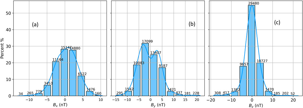
Figure 7. ACE/DSCOVR in situ observations averaged over 20 min. The data are not continuous but selected over seven consecutive years (22 December 2017–30 April 2024). We select the data based on their speed, position of the spacecraft, and ion temperature. The panels (a), (b), and (c) show three components of the magnetic field vector $B_x$, $B_y$, and $B_z$, respectively. Blue solid lines present the kernel density estimation (KDE) of the corresponding datasets.

Figure 8

Figure 8. Distributions of $V_x$ (a), $T_i$ (b), and delay (c) from the ACE/DSCOVR in situ observations averaged over 20 min and selected over seven consecutive years (22 December 2017–30 April 2024). We select the data following the same conditions as in Figure 7. Blue solid lines show KDE distribution as in Figure 7. The scatter plot on panel (d) shows the variations $V_x$ with $T_i$. Color bar depicts the solar wind delay from L1 to the near-Earth location. The black line shows the linear regression line.

For each delay estimation, we employ each variable with 80 data points for the time series data. Therefore, we have $11\times 80$ input feature vectors against one estimated delay. We averaged each input feature data over 80 data points to create one dataset over 20 min. Therefore, averaged data have $11\times 1$ feature vectors for each estimated delay. Figure 7 shows the set of data (averaged over 20 min) for magnetic field components ($B_x$, $B_y$, and $B_z$). Here, the magnetic and velocity components are in GSE coordinates. The solid blue lines show KDE, which uses kernel smoothing for probability density estimation. The mathematical process KDE (O’Brien et al., 2016; Plesovskaya and Ivanov, 2021) is applied to find an estimated probability density function of each dataset.

Figure 8 depicts the $x$ component of the velocity vector $V_{x,GSE}$ [panel (a)], ion temperature $T_i$ [panel (b)], and statistically estimated delay [panel (c)]. The bottom right scatterplot [panel (d)] shows the variation in $V_{x,GSE}$ with the ion temperature $T_i$. Here, the color represents the solar wind delay, and the dashed black line presents the regression line. This color scatterplot shows that the magnitude of the velocity increases with the temperature. The lower right panel also shows that the solar wind delay from L1 to Earth bow shock decreases with increasing proton temperature and speed.

Figure 9a shows the spatial distribution of the positions of MMS and ACE/DSCOVR during the selected time intervals. The L1 spacecraft (ACE/DSCOVR) and near-Earth monitors’ positions in GSE coordinates for the chosen 53,880 events are displayed, where color represents the positions in the Z-direction. Since the aim of this paper is to estimate the propagation time from the L1 spacecraft to the bow shock location, we store the positions of two monitors. Here, the near-Earth monitor represents the bow shock location.

Figure 9

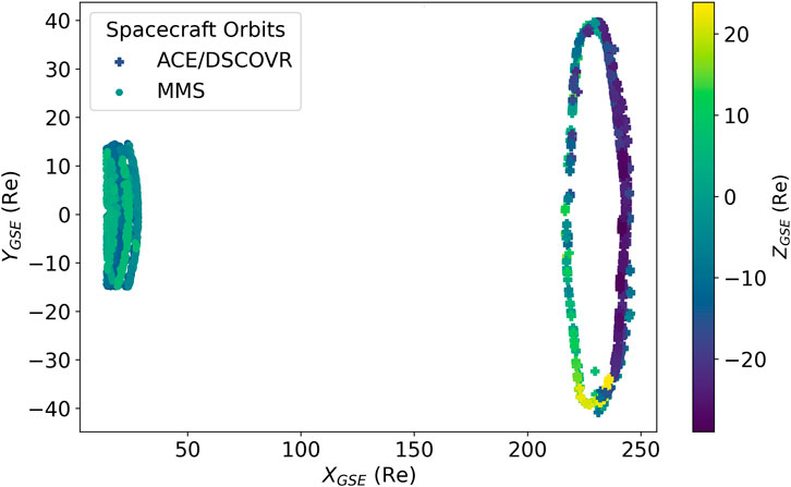
Figure 9. L1 spacecraft (ACE and DSCOVR) and near-Earth monitor’s (MMS) positions in X, Y, and Z (visualized by color) directions in GSE coordinates in Re, where Re is the radius of the Earth. Here, $+$ markers show the ACE/DSCOVR positions, and solid $◦$ markers show the MMS positions.

5 Comparisons with existing methods to compute time delays

To compare the statistical estimations with the OMNI predictions, we need to use the actual distance of the point where the data are shifted. Since the statistical delay is estimated at the near-Earth monitor (e.g., MMS, CLUSTER, and GEOTAIL) location, we need to calculate the time-shift using Equation 2 and use the distance of near-Earth monitors ${\mathbf{R}}_{\mathbf{NE}}$ instead of ${\mathbf{R}}_{\mathbf{B}}$ (location at the Earth’s bow shock nose). Equation 2 can be rewritten as

$\mathrm{\Delta }{t}_{\mathit{OMNI,NE}}=\frac{\mathbf{n}\cdot \left({\mathbf{R}}_{\mathbf{NE}}-{\mathbf{R}}_{\mathbf{O}}\right)}{\mathbf{n}\cdot \mathbf{V}},(14)$

where we employ 1-minute HR data from OMNIWeb. For instance, the phase front normal $\mathbf{n}$ has components ${\mathbf{n}}_{\mathbf{x}}$, ${\mathbf{n}}_{\mathbf{y}}$, and ${\mathbf{n}}_{\mathbf{z}}$, and the solar wind velocity $\mathbf{V}$ has components ${\mathbf{V}}_{\mathbf{x,GSE}}$, ${\mathbf{V}}_{\mathbf{y,GSE}}$, and ${\mathbf{V}}_{\mathbf{z,GSE}}$, and the location of the L1 monitor $R_O$ is given by ${\mathbf{X}}_{\mathbf{GSE}}$, ${\mathbf{Y}}_{\mathbf{GSE}}$, and ${\mathbf{Z}}_{\mathbf{GSE}}$. Note that OMNIWeb time-shifted data are back-shifted to retrieve SW parameters at their origin at L1 monitors. To test our approach, we compare OMNIWeb-provided time-shift at the bow shock nose with the time-shift at the NE location.

Figures 10, 11 compare the statistically estimated delay with the flat delay, the OMNIWeb-provided time-shift at the bow shock, and the calculated time-shift using Equation 14 and OMNIWeb data at the location of near-Earth monitors. Figure 10 shows the results for the ACE–MMS pair. Time delays using different methods are shown in panel (a). OMNI’s offset/time delay at MMS’s location is calculated using OMNI data and Equation 14, which is shown using green markers. We also include the RMS error from OMNIWeb. Note that the OMNIWeb-provided RMS error for the period is $\le 5$ minutes, so the error bars are not easily distinguishable from the markers for most of the cases. We choose three points, namely, $t_1$, $t_2$, and $t_3$, to investigate their features. We select three cases based on the delay difference. We aim to show cases with the largest and smallest difference. The largest difference for the selected period is 5 min. We show two cases of a 5-min difference, one close to the beginning and the other at the end of the selected period. Panels (b), (c), and (d) of Figure 10 show magnetic field components observed by MMS, shifted ACE using statistically estimated delay, and shifted ACE using OMNI data and Equation 14. Each of these panels depicts $B_x$, $B_y$, and $B_z$ for the points $t_1$, $t_2$, and $t_3$. Through visual inspection, we observe that for the selected period (14:00–18:00, 13 December 2017), the statistically estimated delay is more successful in matching the SW IMF features at the L1 point with IMF features at the NE location. Particularly, when the difference between statistical delay and OMNI delay is the highest (at $t_1$), the shifted ACE using statistical delay shows a better match. Since the flat delay or flat plane method was already found to be limited in the various earlier investigations (Ridley, 2000; Horbury et al., 2001; Weimer et al., 2003; Weimer, 2004; Baumann and McCloskey, 2021), we have not included the L1 observations of IMF profiles that were shifted in time according to flat plane propagation in panels (b)–(d) of Figures 10, 11.

Figure 10

Figure 10. [Panel (a)] Comparison of statistically estimated delays (purple) with the corresponding OMNIWeb shifts. Here, the OMNI shift (green) at MMS’s location is calculated using Equation 14 and the OMNIWeb phase normal data. This OMNI shift includes the OMNIWeb-provided root mean squared (RMS) error of time-shift. OMNIWeb provided time-shifts (cyan) at the bow shock and flat delays (black) using Equation 1, which are also shown in panel (a). Magnetic field observed at MMS on the three selected times [$t_1$ (b), $t_2$ (c), and $t_3$ (d)] and the corresponding ACE data lagged by the calculated cross-correlation delay (red) and the OMNI delay (black).

Figure 11

Figure 11. In panel (a), estimated statistical delays (purple) for the DSCOVR–MMS spacecraft pair are compared with the corresponding OMNI shift at MMS’s location with RMS error of time-shift (green), OMNIWeb-provided time-shifts at the bow shock (cyan), and flat delays (black). All of the above delays are calculated using the same method as shown in Figure 10. The observed magnetic field at MMS and the corresponding DSCOVR data lagged by the calculated cross-correlation delay (red) and the OMNI delay (black) are shown for three selected times [$t_1$ (b), $t_2$ (c), and $t_3$ (d)].

A similar comparison between SW delays using various methods is shown in Figure 11: (a) using observations from the DSCOVR–MMS pair for the period 18:00–22:00, 27 December 2017. The shifted magnetic field components for the selected times $t_1$ (b), $t_2$ (c), and $t_3$ (d) indicate that the shifted DSCOVR data using statistically estimated delay match better with the MMS data than that using OMNI’s approach for the selected period. Specifically, upon visual inspection, it can be observed that the OMNI shifted data for $t_2$ and $t_3$ are approximately $\sim 6$ minutes and $\sim 12$ minutes off from the MMS field components, respectively.

Visual inspection of shifted IMF components (from MMS, ACE, and DSCOVR) further supports our findings. Figures 10, 11 and Supporting Figures illustrate several cases with varying levels of discrepancy: some within 5 min and others up to and beyond 20 min. In these cases, our statistical method shows a better match of the time series of magnetic field components between upstream and near-Earth magnetic field features, reinforcing the reliability of our approach.

A quantitative comparison between our statistically estimated delays and OMNIWeb’s predicted propagation delays (Figures 10, 11; Figures 12, 13) reveals generally good agreement, with approximately $95\%$ of the cases showing differences of $\pm 20$ minutes. The vertical green dashed lines in Figure 13 present the $\pm 2\sigma$ range, representing the interval where approximately $95\%$ of the delay differences are expected to lie. We found that, for approximately $80\%$ of the events, OMNIWeb’s delay estimation considering the OMNIWeb uncertainties provides high correlation and aligns with our method. In some cases, we observe significant deviations, with delay differences exceeding 20 min, while the correlation method provides much higher correlation than that using OMNI delay. Values outside this range are considered special cases with significant disagreement between the two methods. Visualizations are provided in the Supporting Figure (Supplementary Figure S1).

Figure 12

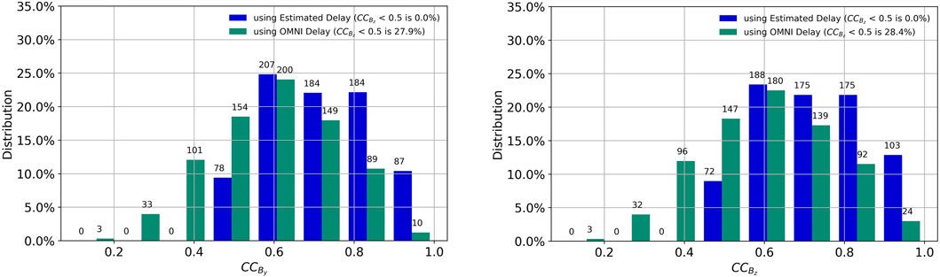
Figure 12. Histograms of the cross-correlation coefficients between DSCOVR and MMS data of $B_y$ (left) and $B_z$ (right). Here, blue bars represent the estimated CC values using the correlation method, and green bars show the results using OMNI’s approach.

Figure 13

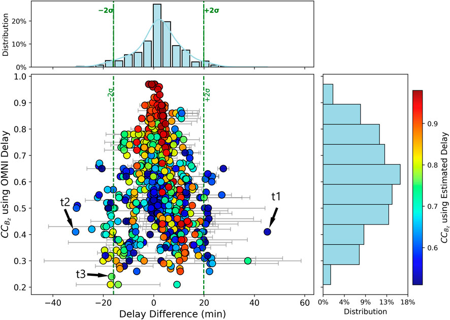
Figure 13. Scatterplot displaying the variation in correlation coefficients $C{C}_{B_z}$ of DSCOVR and MMS data of $B_z$ using OMNIWeb-provided delay with delay difference. The error bars with the delay difference shows the uncertainty provided by OMNIWeb, whereas the color displays $C{C}_{B_z}$. The top sub-panel shows the histogram of differences between statistically estimated delay and calculated delay at the MMS location using Equation 14 and OMNIWeb-provided data. The right sub-panel shows the histogram of $C{C}_{B_z}$ using the estimated delay. The vertical green dashed lines indicate the $\pm 2\sigma$ range of the delay difference.

In panels in Figure 12, the cross-CC values between DSCOVR and MMS observations of $B_y$ (left) and $B_z$ (right) are shown when OMNI data are available, and all required conditions and criteria of data selection in Sections 2, 3.2 are satisfied. To avoid repetition, one event (i.e., a delay data point) is used every 5 min. Here, blue bars show CC values between the 20-min time series magnetic field data of DSCOVR and the corresponding MMS data using statistically estimated delay. For example, if the statistical delay is 50 min, 50 min of delayed MMS data are compared with the DSCOVR data to compute the CC value. For the green bars, the OMNI delays using Equation 14 are employed to calculate the CC values between DSCOVR and MMS. From Figure 12, we found that the correlation coefficient of $B_z$ is slightly higher for both approaches than that of $B_y$; therefore, we use the results of $B_z$ for the comparison.

Figure 12 shows the comparison of the CC values from December 2017 to February 2018. Out of 802 cases (data points) of $B_y$, approximately 100% of the cases result in $CC\ge 0.5$ when using the statistical delay (according to the quality requirement), whereas 72.1% of the cases of OMNI provides similar high $CC$ values. A similar investigation on $B_z$ cases shows that 100% of the cases result in $CC\ge 0.5$ for the statistical delay, and 71.6% of the cases of OMNI delays yield such high CC values. The percentage of correlation coefficient $\le 0.5$ of $B_z$ and $B_y$ are nearly equal using the OMNIWeb method. From the figure, it is clear that the correlation method shows a better correlation than OMNI’s approach for the selected datasets.

The differences between statistically estimated delay and OMNI delay are presented using a histogram in the top panel of Figure 13. In this study, we estimated the results using the DSCOVR and MMS spacecraft pairs. The OMNI delay for DSCOVR–MMS is calculated using Equation 14. The difference between the above two delays/time-shifts is

$\mathrm{\Delta }\text{\hspace{0.17em}Delay}=\text{\hspace{0.17em}Stat.\hspace{0.17em}Delay\hspace{0.17em}}-\text{\hspace{0.17em}OMNI\hspace{0.17em}Delay\hspace{0.17em}}.(15)$

The color scatterplot shows the variation in the calculated correlation coefficient $(C{C}_{B_z})$ using the DSCOVR and MMS data of $B_z$ using OMNI delay with the delay difference ($\mathrm{\Delta }$ delay). The color of the dots represents the calculated CC $(C{C}_{B_z})$ using statistically estimated delay. The vertical green line represents the interval where approximately $95\%$ of the delay differences are expected to lie. The gray error bars display the uncertainties provided by OMNIWeb. The scatterplot shows that where both methods have high $CC$ values, uncertainties are lower. Uncertainties are higher when OMNI has a low $CC$ value, which is consistent with our method. However, we found $18\%$ cases where OMNI has lower $CC$ values than our correlation method, but the OMNI-provided uncertainties are much smaller than the delay values required to obtain the best match. In our estimation, nearly $80\%$ of the cases have a delay difference of $\le 10$ minutes. The light-blue solid curve of the top panel of Figure 13 shows the Gaussian distribution of the data.

Figure 13 shows that our method consistently yields higher correlation values for $B_z$ than that using the OMNIWeb method. We also obtained similar results for $B_y$ (not shown here). We selected three cases (t1, t2, and t3 of Figure 13), with significant delay differences between the two methods and OMNIWeb-provided uncertainties <5 minutes.

The MMS data, along with the shifted L1 data from the statistical method and OMNIWeb, are shown in Supplementary Figure S1. The $\mathrm{\Delta }$ delay is large in all three cases: 45 min (t1), 30 min (t2), and 20 min (t3), respectively. The examples show a comparatively good match using our method, especially in panel (c) components compared to OMNIWeb delays, indicating a more accurate alignment of the IMF. Panels (a) and (b) show that although the correlation method provides higher correlation and a better match than that of OMNI delay, there are differences between magnetic field components that indicate that solar wind changes in traveling from L1 to near-Earth location. In three representative examples, the statistical delay estimates resulted in magnetic field profiles that more closely matched the near-Earth measurements than those obtained using OMNI’s fixed delays.

The expectation is that the data dots should be scattered around the diagonal line, showing that the delay difference increases with increasing uncertainty of OMNIWeb. In addition, it can be expected that the CC (shown in colors) decreases with distance from zero. However, next to this expected distribution of the data in Figure 14, it reveals a significant amount of data in the bottom of the panel, below the orange dash-dotted line. These are the cases when OMNI data are delivered with low uncertainty, but large differences to the statistical delay are detected. Most of these cases where the difference is larger than 5 min have a $CC<0.5$ for the OMNI data, indicating larger uncertainty than the delivered uncertainty. The amount of data points with OMNI uncertainty below 5 min and $\mathrm{\Delta }delay>5$ minutes accumulates to $18\%$.

Figure 14

Figure 14. Variation in absolute values of uncertainties $|\pm \delta |$ provided by OMNIWeb with the absolute delay difference using Equation 15. The green line represents the $|\pm \delta |=|\text{delay\hspace{0.17em}difference}|$ line, whereas the orange line represents the $|\pm \delta |=5$ line. We use the same data as in Figure 13.

Figure 14 displays the variation in uncertainties $(\pm \delta )$ provided by the OMNIWeb and the delay difference. The black dotted box in Figure 14 shows the cases where both the delay difference and the uncertainties are $\le 5$ minutes. Approximately $49\%$ of the selected cases lie inside this box, which indicates that approximately half of our selected cases have an estimation that agrees well with OMNIWeb’s prediction within an uncertainty of $\pm 5$ minutes.

A quantitative comparison is provided in Table 3. According to the comparison, the OMNIWeb delay using Equation 14 provides $C{C}_{B_z}<0.5$ for $29\%$ of cases, whereas the statistical method provides $C{C}_{B_z}\ge 0.5$ for all these cases to maintain the quality requirements. Our analysis reports that OMNIWeb provides better correlation values than our method for $6\%$ of the selected cases. In addition, OMNIWeb provides an uncertainty of $\le |\pm 5|$ minutes for $87\%$ of the cases studied here. The calculated $|\mathrm{\Delta }delay|$ using Equation 15 was $\ge |\pm \delta |$ for $87\%$ of the cases. For approximately $49\%$ cases, $|\mathrm{\Delta }delay|\le 5$, where OMNIWeb-provided uncertainties are reported $|\pm \delta |\le 5$. In approximately $18\%$ of the cases, calculated $C{C}_{B_z}$ is less than 5 min using the OMNIWeb method, where the OMNIWeb-provided uncertainties are $|\pm \delta |\le 5$ minutes, while the delay difference is higher than 5 min.

Table 3

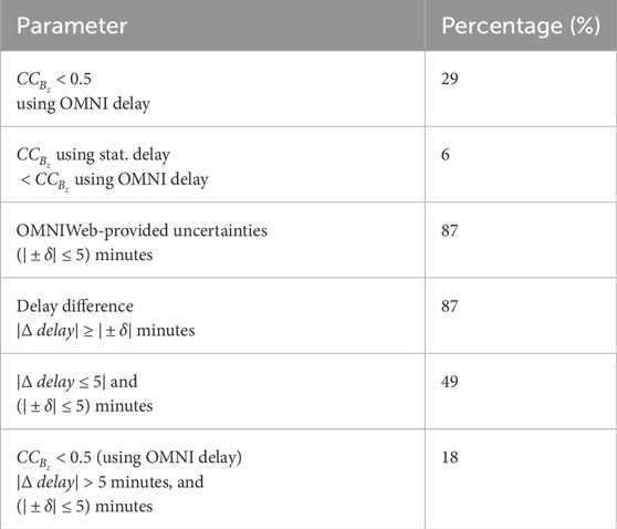
Table 3. Quantitative comparison between OMNI delay and sat. delay over the 802 selected cases.

6 Discussion

The statistical method presented in this work is tested across multiple spacecraft pairs, all showing consistent delay estimates. It performs well for both continuous and discontinuous IMF structures. The statistical analysis using any of the chosen spacecraft pairs of this investigation shows similar results of good matches between estimated delay-shifted IMF components at L1 and near-Earth observations. The correlation method is applicable for both continuous and discrete discontinuities in the IMF. If there is a significant structure or discontinuity, our approach provides a high correlation value and is more likely to match the IMF components at L1 and Earth’s bow shock.

For correlation analysis and SW delay estimations, various lengths of data (data window) have been used previously, from 10 min to a few hours (Crooker et al., 1982; Kelly et al., 1986; Zastenker et al., 2000; Collier et al., 1998; Weimer et al., 2003; Richardson and Paularena, 2001; Weimer and King, 2008; Case and Wild, 2012; Jackel et al., 2013; Vokhmyanin et al., 2019). A too-short period results in high uncertainties of the correlation, while a too-long period is affected by repeating SW structures. We aim to prepare the data appropriately for use as inputs to the prediction models, and the data length should be $<1$ hour to allow advanced prediction. Case and Wild (2012) demonstrated success in using a 10-min period. In our current study, we carried out the analysis over 3 months (December 2017–February 2018) for the periods of 10, 15, 20, and 25 min. We find that those periods of 20-minute-long windows can provide a high correlation coefficient. Compared with the 10-min and 15-min periods, the 20-min period yields better correlation results, although the difference is not substantial. For $14\%$ cases, we obtain $CC<0.5$ using 10-min windows, and for $13\%$ cases, we obtain $CC<0.5$ using 15-min windows, while the use of 20-min windows provides $CC\ge 0.5$ for all those cases. On the other hand, a 25-min window provides slightly ($<5\%$ cases with $CC\ge 0.5$) better estimations than that using 20-min windows, but it reduces the number of good cases. Therefore, we continue our further analysis with a 20-min rolling/sliding window (slides or rolls by 5 min each time) to obtain the highest correlation coefficient and the best model performance.

The correlation analysis using three components of the magnetic field vector is also tested for the selected period (December 2017–February 2018). It is found that estimated delays, using three magnetic components ($B_x$, $B_y$, and $B_z$) in Equation 3 instead of only $B_y$ and $B_z$, provide a very precise match of magnetic field components observed at L1 points and near-Earth location. However, the use of three components to calculate the correlation coefficient $C{C}_{B_{x,y,z}}$ reduces the number of good cases, which becomes significantly lower than when using only two components.

The average of the estimated delay between the observation of the same SW structures at L1 and NE monitors is $55$ minutes using panel (c) of Figure 8, where SW delay varies between 25 min and 100 min depending on features of the solar wind. This estimated average value and the upper and lower limits align with those of the previous studies (Mailyan et al., 2008; Cash et al., 2016). According to Mailyan et al. (2008) and Cash et al. (2016), the SW propagation time/delay is expected to be on the order of 1 h, and the specific value depends closely on the SW conditions. The SW delay varies from over 100 min to less than 30 min (Mailyan et al., 2008; Cash et al., 2016; Baumann and McCloskey, 2021).

The linear regression line of the distribution of solar wind radial velocity and the ion temperature over the 7 years (22 December 2017 to May 2024) in Figure 8 [panel (d)] indicates that the magnitude of the velocity increases with the temperature. This agrees with the long-term linear trend between the solar wind proton temperature and the proton speed observed by Elliott et al. (2016).

The comparison between the estimated delay and the OMNIWeb-provided delay reveals an absolute difference >5 minutes for $48\%$ out of 802 events/cases/data points. This is in good agreement with the predicted delay and observations that were earlier found in Mailyan et al. (2008) and Case and Wild (2012). Mailyan et al. (2008) statistical studies of the solar wind propagation over $198$ events found that the difference is $\ge 5$ min for $\ge 30\%$ of the time. Approximately $40\%$ of the 164 cases presented in Case and Wild (2012) show a delay difference of >5 minutes between the OMNIWeb-provided delay and their estimated delay using correlation analysis (c.f. Figure 11 of Case and Wild, 2012).

In our analysis, we noticed that the delay difference between the estimated delay and the OMNIWeb-provided delay is >20 minutes for $5\%$ cases, with cases where the delay difference is $\ge 30$ minutes. In addition, Mailyan et al. (2008) and Cash et al. (2016) observed delay differences of more than 30 min in individual cases. Importantly, this level of uncertainty does not fully account for the larger observed discrepancies, indicating that in certain conditions, e.g., those involving sudden IMF changes or complex solar wind structures, the OMNI delay may significantly underperform.

The statistical comparison presented in Figure 14 and Table 3 indicates that in approximately $6\%$ of cases, OMNI provides a better $CC$ value than the statistical method presented in this study. These $6\%$ cases are primarily due to the linear interpolation that we apply for the data gap if it is <15 minutes. The fact that $49\%$ of the estimated delays have less than 5 min difference to the OMNI delay and the respective OMNI values have less than 5 min uncertainty indicates that approximately half of the OMNI delays are well-estimated and have very low uncertainty. We also found that approximately $71\%$ of the OMNIWeb-predicted delay provides $CC\ge 0.5$. This result is in agreement with the previous studies of Vokhmyanin et al. (2019) on the data quality in the OMNIWeb IMF field components. They analyzed 10,409 cases over the period 1997–2016 and estimated that approximately $75\%$ of the OMNIWeb data provide reliable predictions based on the conditions $CC\le 0.5$ and prediction efficiency $PE\ge 0$. Approximately $10\%$ of their selected cases have correct variability but wrong absolute values, whereas $15\%$ have poor quality with $CC<0.5$. However, Vokhmyanin et al. (2019) did not consider the uncertainties provided by the OMNIWeb.

Our results showed that there is a fraction of $18\%$ of the cases when the uncertainty of OMNI is below 5 min and the difference in the delay to the statistical method is larger, while the $CC$ is low. These are the cases when OMNI computes wrong SW estimates at the bow shock. For these cases, our method has a higher correlation and a better match between L1 data and NE observation. Earlier research (Crooker et al., 1982; Kelly et al., 1986; Zastenker et al., 2000; Collier et al., 1998; Richardson and Paularena, 2001; Vokhmyanin et al., 2019) on the solar wind and the propagation delay found that the following factors influence the similarity of SW features observed at L1 and upstream of the bow shock: (i) separation of spacecraft in the plane perpendicular to the Sun–Earth line, (ii) the angle between IMF and the GSE X-axis (cone angle), and (iii) evolution of IMF while SW propagates from L1 to near-Earth locations.

When the spacecraft separation is large, the IMF cone angle is small, and/or the IMF variance is low, the similarity between L1 observations and near-Earth SW is likely to be low. Under such conditions, OMNIWeb’s predictions of near-Earth SW features and conditions can have large uncertainties (Crooker et al., 1982; Kelly et al., 1986; Zastenker et al., 2000; Collier et al., 1998; Richardson and Paularena, 2001; Vokhmyanin et al., 2019). OMNIWeb predictions assume that the parameters do not evolve over space and in time, whereas the actual SW is not homogeneous. Thus, OMNIWeb has a particular challenge with dynamic solar wind conditions. In other words, OMNIWeb’s assumption of inhomogeneity in phase front propagation, contrary to the actual solar wind, results in underperformance compared to the statistically estimated solar wind delay. For instance, the solar wind magnetic field components in Supporting Figure (Supplementary Figure S1) are derived from L1 observations rather than those near Earth, which results in significant differences between the statistical estimation and the OMNIWeb prediction. The spacecraft separation, the IMF variance, and the IMF cone angle may also affect the performance of the OMNIWeb predictions (Crooker et al., 1982; Kelly et al., 1986; Zastenker et al., 2000; Collier et al., 1998; Richardson and Paularena, 2001; Vokhmyanin et al., 2019).

The statistical method applied here matches solar wind features as long as the data satisfy the criteria and quality measures, and it considers inhomogeneity in the solar wind and is not limited to the features mentioned above, whereas OMNIWeb does not provide accurate propagation delays or uncertainties. This is the main reason why the statistical method outperforms OMNIWeb in the delay estimation for the selected cases and is an ideal tool to validate OMNIWeb data. However, the feasibility of the method to validate OMNIWeb delay is constrained by the criteria and quality measures. In only $6\%$ of the cases, OMNIWeb provides better $CC$ than the statistical method. These cases are attributed to the data interpolation, which has been applied in this study.

7 Summary and conclusion

In this work, we propose an improved method to estimate the solar wind propagation delay from L1 to Earth’s bow shock location by performing cross-correlation analysis and employing the PMI along with the NDME. We compared delay using different statistical indices and investigated the best combination for estimating delay. Figures 2–6 (and Supplementary Figure S3) display the methodology of the correlation method along with quality measurement and outlier predictions. Because this method is applicable to dynamical solar wind conditions, it is an ideal tool for the validation of OMNIWeb data, which assumes static or homogenous solar wind conditions.

Based on this statistical method, we generated a comprehensive dataset with matching solar wind structures at L1 and near Earth measured by different satellite pairs (e.g., ACE–MMS, ACE–CLUSTER, DSCOVR–MMS, and GEOTAIL–WIND). The estimated delays with the variables, using observations from the ACE–MMS spacecraft pair from 22 December 2017 to 30 April 2024 and the DSCOVR–MMS pair from 22 December 2017 to 31 December 2019, are presented in Figures 7–9 and are publicly available online. The generated datasets provide the chance to employ them to test the respective model predictions and use them in the advancement of near-Earth SW models.

A part of this dataset has been used for the validation of OMNIWeb data. The study compares statistically estimated propagation delays of IMF components with those provided by OMNIWeb (in Figures 10–14), using data from MMS, ACE, and DSCOVR spacecraft. The validation results show that approximately $95\%$ of delay differences between the two methods fall within $\pm 20$ minutes, and $80\%$ of OMNIWeb’s delays are reasonably accurate within their stated uncertainty. Only approximately $50\%$ of the data show very accurate predictions with less than a 5 min difference from the statistical method. Nevertheless, nearly $80\%$ of the OMNIWeb data have a delay difference of 10-min or less compared to the statistical method and are, therefore, reasonably accurate. However, significant discrepancies ($>20$ minutes) are observed in $5\%$ cases. In cases where OMNIWeb provides unreliable results, our improved estimated delays offer a scope for further studies using them as a model input for various models where SW propagation delay from L1 to NE location needs to be addressed, e.g., prediction and forecasting models of $Dst$ and $K_p$.

We acknowledge that the OMNIWeb system remains the most successful in providing spacecraft-specific and non-specific various resolution regular data, and it is widely accepted within the research community and beyond. However, it is possible to minimize the uncertainties in prediction and the adverse effects on space weather operations and forecasts by improving the existing approaches. The results of the statistical method emphasize the value of a dynamic, correlation-based delay estimation method that can adapt to varying solar wind conditions and provide more precise input for space weather modeling and forecasting systems. The dataset generated during this study is publicly available and can be used for further validation and modeling applications.

Table 4

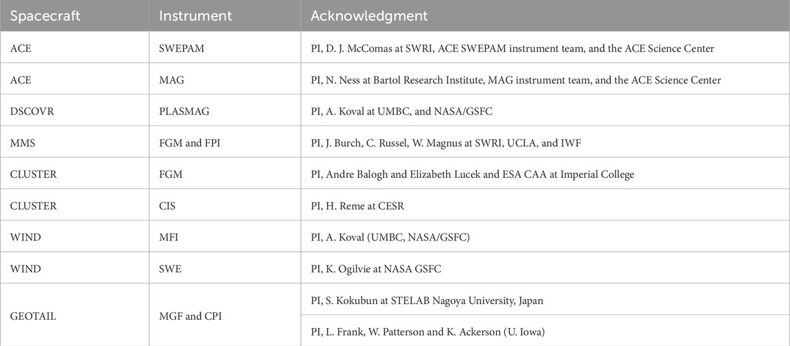
Table 4. Acknowledgment to PIs and the team of the spacecraft and instruments.

Data availability statement

The datasets presented in this study can be found in online repositories. The names of the repository/repositories and accession number(s) can be found at https://zenodo.org/records/17559413, Estimation and assessment of solar wind propagation time from the Lagrange point L1 to Earth's bow shock.

Author contributions

ST: Conceptualization, Data curation, Formal analysis, Investigation, Methodology, Software, Validation, Visualization, Writing – original draft, Writing – review and editing. YZ: Conceptualization, Funding acquisition, Methodology, Project administration, Supervision, Writing – review and editing. ClB: Formal analysis, Supervision, Visualization, Writing – review and editing, Project administration. CaB: Visualization, Writing – review and editing. BW: Conceptualization, Methodology, Writing – review and editing. CO: Visualization, Writing – review and editing. KK: Writing – review and editing. HZ: Writing – review and editing.

Funding

The author(s) declare that financial support was received for the research and/or publication of this article. The authors acknowledge Deutsches Zentrum für Luft-und Raumfahrt (DLR) and NASA grants 80NSSC20K1710 and 80NSSC21K0026 to support this research.

Acknowledgements

The authors are thankful to Arthur Amaral Ferreira for the fruitful discussion. They acknowledge the use of NASA/GSFC’s Space Physics Data Facility’s OMNIWeb (or CDAWeb or ftp) service and OMNI data. Acknowledgments to principle investigators and projects of the instruments used in this manuscript are listed in Table 4.

Conflict of interest

The authors declare that the research was conducted in the absence of any commercial or financial relationships that could be construed as a potential conflict of interest.

Generative AI statement

The author(s) declare that no Generative AI was used in the creation of this manuscript.

Any alternative text (alt text) provided alongside figures in this article has been generated by Frontiers with the support of artificial intelligence and reasonable efforts have been made to ensure accuracy, including review by the authors wherever possible. If you identify any issues, please contact us.

Publisher’s note

All claims expressed in this article are solely those of the authors and do not necessarily represent those of their affiliated organizations, or those of the publisher, the editors and the reviewers. Any product that may be evaluated in this article, or claim that may be made by its manufacturer, is not guaranteed or endorsed by the publisher.

Supplementary material

The Supplementary Material for this article can be found online at: https://www.frontiersin.org/articles/10.3389/fspas.2025.1675769/full#supplementary-material

References

Ashour-Abdalla, M., Walker, R. J., Peroomian, V., and El-Alaoui, M. (2008). On the importance of accurate solar wind measurements for studying magnetospheric dynamics. J. Geophys. Res. Space Phys. 113 (1–16), A08204. doi:10.1029/2007JA012785

CrossRef Full Text | Google Scholar

Baker, D. N., Peterson, W. K., Eriksson, S., Li, X., Blake, J. B., Burch, J. L., et al. (2002). Timing of magnetic reconnection initiation during a global magnetospheric substorm onset. Geophys. Res. Lett. 29, 43. doi:10.1029/2002GL015539

CrossRef Full Text | Google Scholar

Bargatze, L. F., McPherron, R. L., Minamora, J., and Weimer, D. (2005). A new interpretation of Weimer et al.’s solar wind propagation delay technique. J. Geophys. Res. Space Phys. 110, A07105. doi:10.1029/2004JA010902

CrossRef Full Text | Google Scholar

Baumann, C., and McCloskey, A. E. (2021). Timing of the solar wind propagation delay between l1 and Earth based on machine learning. J. Space Weather Space Clim. 11, 41. doi:10.1051/swsc/2021026

CrossRef Full Text | Google Scholar

Bhattacharjee, G. P., and Mohan, R. (1963). Dimensional chains involving rectangular and normal error-distributions. Technometrics 5, 404–406. doi:10.2307/1266346

CrossRef Full Text | Google Scholar

Borovsky, J. E. (2010). On the variations of the solar wind magnetic field about the parker spiral direction. J. Geophys. Res. 115, A09101. doi:10.1029/2009JA015040

CrossRef Full Text | Google Scholar

Cameron, T., and Jackel, B. (2016). Quantitative evaluation of solar wind time-shifting methods. Space Weather 14, 973–981. doi:10.1002/2016sw001451

CrossRef Full Text | Google Scholar

Case, N. A., and Wild, J. A. (2012). A statistical comparison of solar wind propagation delays derived from multispacecraft techniques. J. Geophys. Res. 117, A02101. doi:10.1029/2011JA016946

CrossRef Full Text | Google Scholar

Cash, M. D., Hicks, S. W., Biesecker, D. A., Reinard, A. A., de Koning, C. A., and Weimer, D. R. (2016). Validation of an operational product to determine l1 to Earth propagation time delays. Space Weather 14, 93–112. doi:10.1002/2015SW001321

CrossRef Full Text | Google Scholar

Collier, M. R., Slavin, J. A., Lepping, R. P., Szabo, A., and Ogilvie, K. (1998). Timing accuracy for the simple planar propagation of magnetic field structures in the solar wind. Geophys. Res. Lett. 25, 2509–2512. doi:10.1029/98GL00735

CrossRef Full Text | Google Scholar

Crooker, N. U., Siscoe, G. L., Russell, C. T., and Smith, E. J. (1982). Factors controlling degree of correlation between isee 1 and isee 3 interplanetary magnetic field measurements. J. Geophys. Res. 87, 2224–2230. doi:10.1029/JA087iA04p02224

CrossRef Full Text | Google Scholar

Elliott, H. A., McComas, D. J., and DeForest, C. E. (2016). Long-term trends in the solar wind proton measurements. Astrophys. J. 832, 66. doi:10.3847/0004-637X/832/1/66

CrossRef Full Text | Google Scholar

Farris, M. H., and Russel, C. T. (2017). Determining the standoff distance of the bow shock: Mach number dependence and use of models. J. Geophys. Res. 99, 17681–17690. doi:10.1029/94JA01020

CrossRef Full Text | Google Scholar

Ferreira, A. A., Borries, C., Xiong, C., Borge, R. A., Mielich, J., and Kouba, D. (2020). Identification of potential precursors for the occurrence of large-scale traveling ionospheric disturbances in a case study during september 2017. J. Space Weather Space Clim. 10, 32. doi:10.1051/swsc/2020029

CrossRef Full Text | Google Scholar

Fredrick, E., Hong, Y., Lopez, R., and Deng, Y. (2025). The impact of OMNI data accuracy on thermospheric neutral density simulations at grid cell resolutions. J. Geophys. Res. 23, e2025SW004374. doi:10.1029/2025SW004374

CrossRef Full Text | Google Scholar

Haaland, S., Paschmann, G., and Sonnerup, B. U. Ö. (2006). Comment on “a new interpretation of Weimer et al.’s solar wind propagation delay technique” by Bargatze et al. J. Geophys. Res. 111, A06102. doi:10.1029/2005JA011376

CrossRef Full Text | Google Scholar

Haaland, S., Munteanu, C., and Mailyan, B. (2010). Solar wind propagation delay: comment on “Minimum variance analysis-based propagation of the solar wind observations: application to real-time global magnetohydrodynamic simulations” by A. Pulkkinen and L. raststätter: COMMENTARY. Space Weather 8, 06005. doi:10.1029/2009SW000542

CrossRef Full Text | Google Scholar

Horbury, T. S., Burgess, D., Fränz, M., and Owen, C. J. (2001). Prediction of Earth arrival times of interplanetary southward magnetic field turnings. J. Geophys. Res. 106, 30001–30009. doi:10.1029/2000JA002232

CrossRef Full Text | Google Scholar

Jackel, B. J., Cameron, T., and Weygand, J. M. (2013). Orientation of solar wind dynamic pressure phase fronts. J. Geophys. Res. Space Phys. 118, 1379–1388. doi:10.1002/jgra.50183

CrossRef Full Text | Google Scholar

Kelly, T. J., Crooker, N. U., Siscoe, G. L., Russell, C., and Smith, E. J. (1986). On the use of a sunward libration-point-orbiting spacecraft as an interplanetary magnetic field monitor for magnetospheric studies. J. Geophys. Res. 91, 5629–5636. doi:10.1029/JA091iA05p05629

CrossRef Full Text | Google Scholar

Knetter, T., Neubauer, F. M., Horbury, T., and Balogh, A. (2004). Four-point discontinuity observations using cluster magnetic field data: a statistical survey. J. Geophys. Res. Space Phys. 109, A06102. doi:10.1029/2003JA010099

CrossRef Full Text | Google Scholar

Lethy, A., El-Eraki, M. A., Samy, A., and Deebes, H. A. (2018). Prediction of the dst index and analysis of its dependence on solar wind parameters using neural network. Space Weather 16, 1277–1290. doi:10.1029/2018SW001863

CrossRef Full Text | Google Scholar

Lotz, S. I., Heyns, M., and Cilliers, P. J. (2017). Regression-based forecast model of induced geoelectric field. Space Weather 15, 180–191. doi:10.1002/2016SW001518

CrossRef Full Text | Google Scholar

Lyons, L. R., and Nishimura, Y. (2020). Substorm onset and development: the crucial role of flow channels. J. Atmos. Sol. Terr. Phys. 211, 105474. doi:10.1016/j.jastp.2020.105474

CrossRef Full Text | Google Scholar

Mailyan, B., Munteanu, C., and Haaland, S. (2008). What is the best method to calculate the solar wind propagation delay? Ann. Geophys. 26, 2383–2394. doi:10.5194/angeo-26-2383-2008

CrossRef Full Text | Google Scholar

Mineo, A. M., and Ruggieri, M. (2005). A software tool for the exponential power distribution: thenormal package. J. Stat. Softw. 12, 1–24. doi:10.18637/jss.v012.i04

CrossRef Full Text | Google Scholar

Munteanu, C., Haaland, S., Mailyan, B., Echim, M., and Mursula, K. (2013). Propagation delay of solar wind discontinuities: comparing different methods and evaluating the effect of wavelet denoising. J. Geophys. Res. Space Phys. 118, 3985–3994. doi:10.1002/jgra.50429

CrossRef Full Text | Google Scholar

O’Brien, T. A., Kashinath, K., Cavanaugh, N. R., Collins, W. D., and O’Brien, J. P. (2016). A fast and objective multidimensional kernel density estimation method: fastKDE. Comput. Stat. Data Anal. 101, 148–160. doi:10.1016/j.csda.2016.02.014

CrossRef Full Text | Google Scholar

Plesovskaya, E., and Ivanov, S. (2021). An empirical analysis of KDE-Based generative models on small datasets. Procedia Comput. Sci. 193, 442–452. doi:10.1016/j.procs.2021.10.046

CrossRef Full Text | Google Scholar

Pontius, R. G., Thontteh, O., and Chen, H. (2008). Components of information for multiple resolution comparison between maps that share a real variable. Environ. Ecol. Stat. 15, 111–142. doi:10.1007/s10651-007-0043-y

CrossRef Full Text | Google Scholar

Pulkkinen, A., and Rastätter, L. (2009). Minimum variance analysis-based propagation of the solar windobservations: application to real-time global magnetohydrodynamic simulations. Space Weather 7, S12001. doi:10.1029/2009SW000468

CrossRef Full Text | Google Scholar

Pulkkinen, A., Kuznetsova, M., Ridley, A., Raeder, J., Vapirev, A., Weimer, D., et al. (2011). Geospace environment modeling 2008–2009 challenge: ground magnetic field perturbations. Space Weather 9, 02004. doi:10.1029/2010SW000600

CrossRef Full Text | Google Scholar

Richardson, J. D., and Paularena, K. I. (2001). Plasma and magnetic field correlations in the solar wind. J. Geophys. Res. Space Phys. 106, 239–251. doi:10.1029/2000JA000071

CrossRef Full Text | Google Scholar

Ridley, A. J. (2000). Estimations of the uncertainty in timing the relationship between magnetospheric and solar wind processes. J. Atmos. Sol. Terr. Phys. 62, 757–771. doi:10.1016/S1364-6826(00)00057-2

CrossRef Full Text | Google Scholar

Roble, R. G., and Ridley, E. C. (1994). A thermosphere-ionosphere-mesosphere-electrodynamics general circulation model (time-gcm): equinox solar cycle minimum simulations (30-500 km). Geophys. Res. Lett. 21, 417–420. doi:10.1029/93GL03391

CrossRef Full Text | Google Scholar

Shue, J.-H., Chao, J. K., Fu, H. C., und, P., Song, C. T. R., Khurana, K. K., et al. (1997). A new functional form to study the solar wind control of the magnetopause size and shape. J. Geophys. Res. 102, 9497–9511. doi:10.1029/97JA00196

CrossRef Full Text | Google Scholar

Tsurutani, B. T., Guarnieri, F. L., Lakhina, G. S., and Hada, T. (2005). Rapid evolution of magnetic decreases (MDs) and discontinuities in thesolar wind: ace and cluster. Geophys. Res. Lett. 32, L10103. doi:10.1029/2004GL022151

CrossRef Full Text | Google Scholar

Vokhmyanin, M. V., Stepanov, N. A., and Sergeev, V. A. (2019). On the evaluation of data quality in the omniinterplanetary magnetic field database. Space Weather 17, 476–486. doi:10.1029/2018sw002113

CrossRef Full Text | Google Scholar

Watterson, I. G. (1996). Non-dimensional measures of climate model performance. Int. J. Climatol. 16, 379–391. doi:10.1002/(SICI)1097-0088(199604)16:4⟨379::AID-JOC18⟩3.0.CO;2-U

CrossRef Full Text | Google Scholar

Weimer, D. R. (2004). Correction to “predicting interplanetary magnetic field (imf) propagation delay times using the minimum variance technique”. J. Geophys. Res. 109, A12104. doi:10.1029/2004JA010691

CrossRef Full Text | Google Scholar

Weimer, D. R., and King, J. H. (2008). Improved calculations of interplanetary magnetic field phase front angles and propagation time delays. J. Geophys. Res. 113, A01105. doi:10.1029/2007JA012452

CrossRef Full Text | Google Scholar

Weimer, D. R., Ober, D. M., Maynard, N. C., Collier, M. R., McComas, D. J., Ness, N. F., et al. (2003). Predicting interplanetary magnetic field (Imf) propagation delay times using the minimum variance technique. J. Geophys. Res. Space Phys. 108. doi:10.1029/2002JA009405

CrossRef Full Text | Google Scholar

Willmott, C. J., Robeson, S. M., and Matsuura, K. (2012). A refined index of model performance. Int. J. Climatol. 32, 2088–2094. doi:10.1002/joc.2419

CrossRef Full Text | Google Scholar

Wintoft, P., Wik, M., Matzka, J., and Shprits, Y. (2017). Forecasting kp from solar wind data: input parameter study using 3-hour averages and 3-hour range values. J. Space Weather Space Clim. 7, A29. doi:10.1051/swsc/2017027

CrossRef Full Text | Google Scholar

Wu, C., Fry, C. D., Berdichevsky, D., Smith, Z., and Detman, T. (2005). Predicting the arrival timeof shock passages at Earth. Sol. Phys. 227, 371–386. doi:10.1007/s11207-005-1213-4

CrossRef Full Text | Google Scholar

Zastenker, G. N., Dalin, P. A., Petrukovich, A. A., Nozdrachev, M., Romanov, S., Paularena, K., et al. (2000). Solar wind structure dynamics by multipoint observations. Phys. Chem. Earth, Part C Sol. Terr. and Planet. Sci. 25, 137–140. doi:10.1016/S1464-1917(99)00055-0

CrossRef Full Text | Google Scholar