Lower-thermospheric vertical wind measurements from the Arecibo radio observatory

Vertical wind profiles in the lower thermosphere computed from data from the Arecibo Radio Observatory between 2013 and 2016 are reviewed and analyzed. The estimates are derived from ion-line spectral measurements in the E and F regions made with the Arecibo dual-beam incoherent scatter radar using a number of specialized pulsing schemes. The background electric field is estimated on the basis of F-region samples, and its effects are then removed from E-region samples. Statistical inverse methods are used to estimate vector wind profiles in the lower thermosphere versus time. Data from the daytime E region and from nighttime sporadic- E layers are examined. We find large and highly variable vertical winds in the lower thermosphere at upper E-region altitudes. Frequency and vertical wavenumber spectra computed from the vertical wind estimates exhibit power laws, and the latter exhibit some degree of universality. The spectral forms are consistent with those measured in the mesosphere elsewhere. Theoretical interpretations of the spectral measurements are briefly reviewed.

1 Introduction

The mesosphere/lower thermosphere (MLT) is one of the most dynamically complex regions in the atmosphere. Vertical transport is important in all parts of the atmosphere because of the larger gradients along the vertical at all heights, but is especially important in the MLT region where the very nature of the dynamics changes significantly as a function of height. Across the turbopause boundary that occurs somewhere between 100 and 105 km, there is a sharp transition from well-mixed turbulent flow to diffusively-separated more laminar flow. The ionized component of the atmosphere also plays an increasingly important role with increasing altitude in that height range, transitioning from an essentially passive trace component to a component with behavior distinct from the neutrals that can actually affect and modify the neutral dynamics. Furthermore, there are important minor constituents, such as neutral and ion metallic layers with densities that vary strongly with height and can change the electrodynamics and plasma physics of the region. In spite of the importance of the vertical winds and associated vertical transport effects, obtaining vertical velocity measurements at MLT heights has been difficult. Nearly all of the available measurements are from altitudes below 100 km, i.e., in the mesosphere.

In general, neutral winds in the lower thermosphere shape the state of the upper atmosphere, modifying energetics, dynamics, and transport locally and globally, promoting and inhibiting atmospheric waves propagating upward, driving dynamo electric fields and currents, and disposing the E- and F-region ionosphere to plasma instability. Wind measurements are notoriously difficult to make in the lower thermosphere, however, especially when long time series and fine spatial and temporal resolutions are required. Meteor and medium frequency (MF) radar techniques are limited mainly to altitudes below 100 km. Green-line airglow observations can be used to estimate lower thermospheric winds, but accurate altitude profiling generally requires common-volume triangulation measurements, and measurements throughout the entire day are often impractical. Resonance lidar measurements are limited to the altitudes where scattering layers are present. Rocket measurements using neutral tracers such as trimethyl aluminum provide excellent altitude coverage and height resolution but are limited to snapshot views at a particular time and location. In any case, estimates of the vertical winds require high-accuracy measurements and pose additional practical challenges. In this paper we present inferred neutral vertical wind estimates extending above 100-km altitude up to 130 km, an altitude range where very few such measurements exist.

Prior to its demise at the end of 2020, the Arecibo Radio Observatory was the most sensitive radar in the world capable of observing collective Thomson scatter (incoherent scatter) from the ionosphere (Campbell, 2024). The method can be used to estimate the most important ionospheric state parameters in the D, E, and F regions. Among these are plasma number density, electron and ion temperature, ion composition, and line-of-sight ion drift. While neutral atmospheric state parameters cannot be measured directly with incoherent scatter, neutral winds may be inferred from a combination of ionospheric parameter estimates at altitudes below about 170 km where plasma diffusion in the direction parallel to the magnetic field can be neglected (Vasseur, 1969; Behnke and Kohl, 1974). Inferring vector neutral winds from plasma drifts becomes practical below an altitude of about 130 km where the ions become partially magnetized (Harper et al., 1976).

The accuracy and precision of ISR techniques prompt an investigation of their application to neutral dynamics measurements in the lower thermosphere. Wind measurements in the mesosphere and below using high-power, large aperture radars at VHF frequencies and above are also possible and relatively straightforward where the ions are unmagnetized and line-of-sight drift measurements are essentially neutral drift measurements. However, mesosphere-stratosphere-troposphere (MST) radar techniques represent a distinct field of study involving specialized practices and capabilities (Woodman and Guillén, 1974).

The ISR methods used for neutral-wind estimation in the lower thermosphere were summarized by Harper (1977) and references therein. They involve posing the momentum equation for the ions in the lower thermosphere and solving for the winds that are most consistent with whatever line-of-sight ion velocity measurements are available. This approach is straightforward but has three significant complications. The first is that the ionospheric electric field appears in the momentum equation and requires its own method of estimation. The second is that the ion composition has to be estimated, both for using the momentum equation and while making temperature measurements, but composition cannot be determined uniquely in the lower thermosphere on the basis of incoherent scatter (ISR) theory alone due to isomorphism in the spectrum. The third and gravest problem is that the resulting system of equations for the neutral winds is generally rank deficient and possibly poorly conditioned in practice. This means that the wind solution is likely to be unstable and require some form of regularization which will inevitably restrict the solution space in some way. At the very least, a number of assumptions regarding the stationarity and homogeneity of the state parameters being measured and estimated are required.

The electric field is typically assumed to be stationary and homogeneous and estimated on the basis of F-region ion drift-velocity measurements. Here, the drifts are assumed to be $\mathbf{E}\times \mathbf{B}$ drifts, simplifying their interpretation. Measuring F-region line of sight drifts with the ISR technique is still challenging at middle and low latitudes, however, since typical drift speeds are very small compared to the width of the incoherent scatter spectrum at most magnetic aspect angles. The accuracy of the measurements has to be rather good, and the experimental cadence has to be rather rapid to facilitate useful wind measurements in practice. The Arecibo Radio Observatory was ideal in view of its unsurpassed sensitivity.

Experimentally, it is expedient to combine data from multiple pulse patterns optimized separately for E- and F-region measurements. Harper (1977) used a multipulse pattern to measure E-region autocorrelation functions and long pulses to measure F-region line-of-sight drift velocities. More recent work at Arecibo replaced the multipulse with a coded long pulse (CLP) and the long pulse experiment with either the CLP or the “MRACF” mode which combined statistically independent data from multiple, closely-spaced radar frequencies. These refinements improved experimental precision and accuracy substantially. For a review of these methods, see Sulzer (1986a), Sulzer (1986b).

Simultaneous ion temperature and composition measurements generally require some assistance from modeling in the lower thermosphere where atomic and molecular ions coexist. When winds are estimated at night, sporadic E layers are required for a source of E region backscatter. In this case, the main ion constituents are metallic ions. Fitting for ion composition in this case may be performed provided that the candidate ions have dissimilar atomic masses.

Ambiguity in wind field estimation can be reduced by incorporating information from multiple beams. Starting in 1996, dual beam systems became available at Arecibo, greatly improving the efficacy of the winds methods. However, the problem remains underdetermined with dual beams, and regularization is generally required. Regularization methods were introduced at Arecibo by Sulzer et al. (2005) and at EISCAT by Nygrén et al. (2011). Hysell et al. (2014) applied regularization methods to the underdetermined wind-field estimation problem, exploiting the aforementioned Arecibo upgrades in order to include vertical winds.

In this paper, we revisit Arecibo vertical wind data acquired in 2013, 2015, and 2016 and published separately (Hysell et al., 2014; 2016; 2018). The focus of the earlier studies was on the horizontal winds and the tendency for dynamic instability leading to ionospheric structuring. The objective now is both to review the methodology and summarize the findings of experiments that cannot presently be repeated. Vertical winds in the daytime and nighttime lower thermosphere are found to be large and highly variable as a rule for sustained time intervals. We examine the frequency and vertical wavenumber spectra of the vertical winds and compare their behavior with other measurements in the literature.

2 Arecibo methodology

Lower thermospheric wind estimates were calculated from Arecibo Coordinated World-Day data starting in 2013. These data comprised ion-line measurements in combined CLP and MRACF modes using Arecibo’s dual feed (Gregorian and linefeed) system. One feed was directed at zenith, and the other at 15$°$ zenith angle and swept in azimuth. The azimuth slew rate was about 25$°$ per minute. The fundamental measurement cadence was once every 30, 40, or 60 s depending on the specific mode in use. Range resolution was 300 m. The half power full beamwidth of the UHF radar was approximately 10’.

We consider first the estimation of the ionospheric electric field from F-region line-of-sight ion drift measurements. Following Hysell et al. (2014) and assuming that the F-region ion drifts are spatially uniform, the unknown ion velocities in local magnetic coordinates are related to the line-of-sight drifts measured with the dual feeds through a time-dependent linear transformation, viz.

$V_{dF}={⌈\begin{array}{c}\hfill v_l\hfill \\ \hfill v_g\hfill \end{array}⌉}_F=S\left(\theta ,\varphi \right){⌈\begin{array}{c}\hfill v_{\Vert }\hfill \\ \hfill v_{\perp e}\hfill \\ \hfill v_{\perp n}\hfill \end{array}⌉}_F=S{V}_{lF}(1)$

where $v_l$ and $v_g$ in Equation 1 refer to drifts measurements from the dual line feed and Gregorian feed system and $v_{\Vert }$, $v_{\perp e}$, and $v_{\perp n}$ are the local drift components parallel to $B$, perpendicular to $B$ and eastward, and perpendicular to $B$ and northward. The angles $\theta$ and $\varphi$ are the azimuth and zenith angles of the off-zenith feed. The transformation matrix $S$ also depends on the inclination and declination of the magnetic field. If measurements at $n$ times are available, then $V_{dF}$, $V_{lF}$, and $S_F$ can be generalized from ${\mathbb{R}}^2$, ${\mathbb{R}}^3$, ${\mathbb{R}}^{2\times 3}$, respectively, to the band diagonal system ${\mathbb{R}}^{2n}$, ${\mathbb{R}}^{3n}{\mathbb{R}}^{2n\times 3n}$.

The transformation $S$ is under determined and cannot be inverted directly. Estimating the drifts in local magnetic components from dual-beam drifts measurements is performed by minimizing an objective function incorporating the $\chi$-square parameter and a regularization penalty. The Moore-Penrose pseudoinverse for linear systems can be used here.

${\widehat{V}}_{lF}=\underset{V_{lF}}{\mathrm{arg\; min}}{\left(S_F{V}_{lF}-V_{dF}\right)}^t{C}_d^{-1}\left(S_F{V}_{lF}-V_{dF}\right)+{\alpha }^2{V}_{lF}^t{W}_F{V}_{lF}(2)$

$={\left(S_F^t{C}_d^{-1}{S}_F+{\alpha }^2{W}_F\right)}^{-1}{S}_F^t{C}_d^{-1}{V}_{dF}(3)$

where $C_d$ in Equation 2 is the data error covariance matrix for the ISR measurements, $\alpha$ is the regularization parameter, and $W_F$ is the weight matrix that penalizes the curvature in the estimates (i.e., Second-order Tikhonov regularization) (see e.g., Aster et al., 2005). In practice, the regularization parameter can be set such that the $\chi$-squared term in Equation 2 has the expected value of $\chi$-squared for the appropriate number of degrees of freedom.

We turn next to wind field estimation. It is not necessary to resolve the components of the electric field from the F-region drift measurements. Instead, we assume that the electric field is the same in the E and F region and use the measurements from the latter to inform or ‘correct’ the former. Neglecting the effects of pressure, inertia, and gravity, and assuming that the parallel electric field is also negligibly small, ion drifts are related to neutral winds and electric fields by the following expression

$\mathbf{V}=\frac{r^2}{1+r^2}{\mathbf{U}}_{\perp }+\frac{r}{1+r^2}\mathbf{U}\times \mathbf{B}+\mathbf{U}\cdot \widehat{b}\widehat{b}+\frac{r}{1+r^2}\frac{{\mathbf{E}}_{\perp }}{B}+\frac{1}{1+r^2}\frac{1}{B}\mathbf{E}\times \widehat{b}(4)$

where $\widehat{b}$ is a unit vector in the direction of the geomagnetic field $\mathbf{B}$ and $r={\nu }_{in}/{\mathrm{\Omega }}_i$ is the ratio of the ion neutral collision frequency to the ion gyrofrequency. In the F region with the approximation $r\sim 0$, the significant term in Equation 4 is the $\mathbf{E}\times \mathbf{B}$ drift term. Drifts measurements in local magnetic coordinates in the F region can therefore be used to populate Equation 4 in the E region which can be reformulated and solved for the Cartesian components of the neutral winds U.

Accordingly, Equation 4 can be formulated in the E region in local magnetic coordinates in matrix form as:

$V_{lE}-Q{V}_{lF}=R{U}_{lE}(5)$

where the matrices $Q$ and $R$ incorporate the ratio $r$ appropriate in the E region. The matrix $Q$ converts the electrical mobility from F to E region conditions, and the matrix $R$ prescribes the drifts that result from E-region winds. Multiplying by the transformation $S$ and rearranging yields:

$\left(SR\right)U_{lE}=\left(V_{dE}-SQ{\widehat{V}}_{lF}\right)(6)$

which gives the prescription for evaluating the E region lower thermospheric winds in local magnetic coordinates on the basis of the dual feed line-of-sight drifts measurements supported by precomputed estimates of the ratio $r$. Note that the rightmost term in Equation 6 above is like $SQ{S}^{-1}{V}_{dF}$ involving $Q$ transformed into dual-beam space except with $S^{-1}$ being the pseudoinverse of $S$.

As the electric fields are regarded as being spatially uniform, line-of-sight drifts measurements in the F region are averaged in altitude to improve statistics. The CLP measurements in the E region are range resolved, of course, and $r$ is a function of altitude. Given $m$ samples in range and $n$ samples in time, the dimensionality of the coefficient matrices in Equation 5 are consequently $V_{lE}\in {\mathbb{R}}^{3nm\times }$, $U_{lE}\in {\mathbb{R}}^{3nm\times }$, $Q\in {\mathbb{R}}^{3nm\times 3n}$, $R\in {\mathbb{R}}^{3nm\times 3nm\times }$, and $S\in {\mathbb{R}}^{2nm\times 3nm\times }$. The specific elements of the matrices $Q$, $R$, and $S$ are given in Hysell et al. (2014).

Finally, the inverse implied in Equation 6 could be performed using the Moore-Penrose pseudoinverse once again, second-order Tikhonov regularization being introduced through an additional weight matrix $W_E$ to penalize curvature. However, due to the size of the design matrix, this would be very computationally costly. We therefore use the method of conjugate gradients least squares (CGLS), exploiting sparse matrix math to reduce the cost substantially. This is an iterative method that involves nothing more expensive than matrix vector multiplications (a Krylov method).

Specifically, writing the underdetermined problem in Equation 6 as $AX=Y$ where $X\in {\mathbb{R}}^{3nm\times }$ is the neutral wind estimate, we use CGLS to solve the augmented, weighted, damped system.

${\tilde{A}}^t\tilde{A}X={\tilde{A}}^t\tilde{Y}(7)$

$\tilde{A}\equiv ⌈\begin{array}{c}\hfill C_d^{-1/2}A\hfill \\ \hfill \alpha W_E^{1/2}\hfill \end{array}⌉(8)$

$\tilde{Y}\equiv ⌈\begin{array}{c}\hfill C_d^{-1/2}Y\hfill \\ \hfill 0\hfill \end{array}⌉(9)$

Equations 7–9 are just a generalization of the pseudoinverse given in Equation 2. Here, the data error covariance matrix and the regularization weight matrix are positive definite, and the regularization parameter $\alpha$ is again adjusted such that the $\chi$-squared parameter takes on its expected value. Regularization is applied both in space and in time. The starting point for iteration is the null solution.

Calculating $r(h)$ as a function of altitude and weighted by ion fractional number density requires an empirical model of the geomagnetic field, the composition of the neutral atmosphere, and estimates of the ion temperature and composition which fix the net ion-neutral collision frequency and gyro-frequency. The magnetic field and neutral atmosphere models used are the International Geomagnetic Reference Field (IGRF) and the Mass Spectrometry Incoherent Scatter (MSIS) model, respectively, which undergo regular revision (Thébault et al., 2015; Emmert et al., 2021). Ion temperature can be estimated from the shape of the ion line using standard ISR techniques but not in the E region in the daytime where atomic and molecular ion species cannot be differentiated. During the daytime, we estimate ion composition by imposing chemical equilibrium (e.g., Richards et al. (2010)). At night, the ionization layers in question are sporadic E layers composed of metallic ions. Our practice has been to fit the ISR spectrum for temperature and composition together assuming a mixture of heavy (iron) and light (calcium) ions. Once the temperature and composition profiles are found, the ion-neutral collision frequencies can be determined using the expressions given in Schunk and Nagy (2004).

3 Vertical wind observations

Vertical wind estimates from three different Coordinated World Day experiments in 2013, 2014, and 2015 are shown in Figure 1. The first two examples (2013, 2014) correspond to daytime measurements of the usual E layers while the third example (2015) corresponds to nighttime measurements from a long-lived, vertically-extended sporadic E layer. The lengths of the time series involved are relatively short and grow progressively shorter from 2013 to 2014 to 2015. While the time series are too short to identify tidal periods, they are nonetheless many times the nominal buoyancy period in the lower thermosphere.

Figure 1

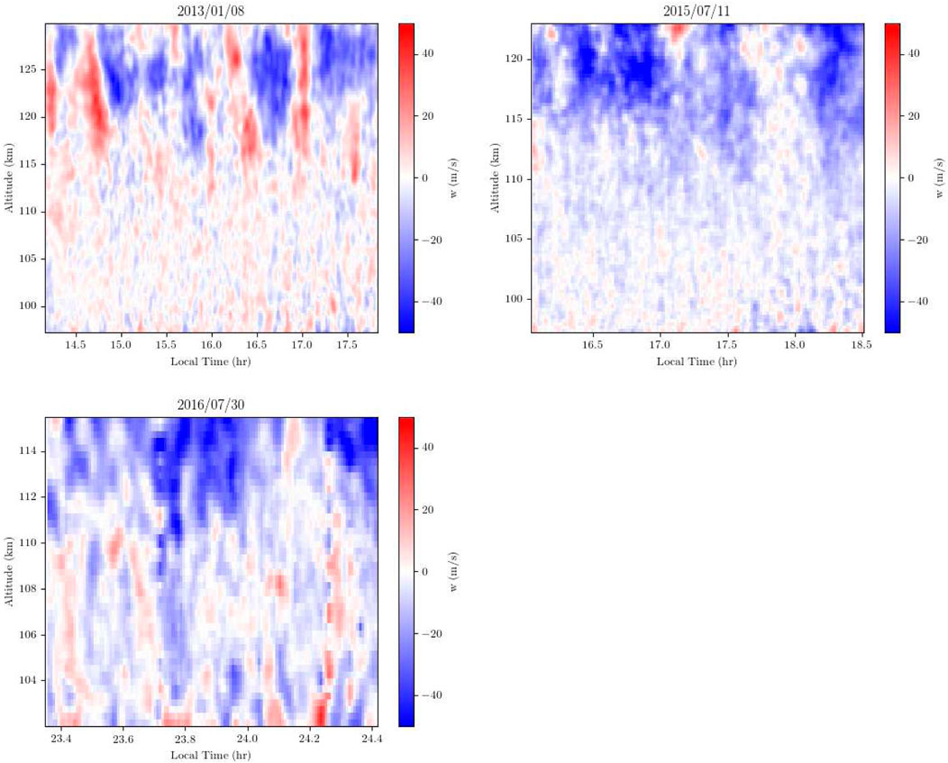
Figure 1. Vertical wind speeds versus altitude and local time estimated for three different Arecibo Coordinated World Day runs in 2013, 2014, and 2015. The top row corresponds to daytime measurements, and the bottom row to nighttime measurements in a broad sporadic E layer. Positive vertical wind speed implies ascent.

While hardly a comprehensive dataset, the vertical winds have some characteristics in common as well as some notable differences. Common to all the datasets is the tendency for the wind amplitudes to increase with altitude from about $\pm$10 m/s at 100 km to as much as $\pm$50 m/s at 125 km altitude. The largest winds, which occur above 115-km altitude, alternate between upward and downward in the 2013 dataset. Note that there are periods of sustained winds that last 30 min or longer. The vertical velocities are preferentially downward in the 2015 and 2016 datasets. Notably, the 2015 dataset exhibits large, nearly sustained downward winds for an interval of about 2.5 h. All three data sets show a notable increase in the velocities at the upper altitudes. The transition occurs above 115 km in the daytime samples, and at a lower altitude of $\sim$110 km in the nighttime data. Note that the 2016 dataset exhibits relatively large vertical winds over its altitude span of 102–116 km. As these measurements correspond to a patchy sporadic E layer with unusually broad vertical development, it is perhaps not surprising for the vertical winds to be especially large in view of the fact that the layer was unstable in the Richardson-number sense and a strong candidate for Kelvin Helmholtz instability (Hysell et al., 2016).

The vertical winds also exhibit long vertical correlation lengths. The temporal behavior, meanwhile, appears almost periodic at times. This could be telltale of coherent underlying waves or eddies embedded in a high-order statistical flow.

Note that vertical ion drift estimates for the datasets shown in Figure 1 were presented previously (Hysell et al., 2014; 2016; 2018). Below about 115 km altitude, the vertical winds and vertical plasma drifts resembled one another fairly closely. Between about 115 and 125 km altitude, the ions ascended, and above 125 km, they descended. The low, middle, and high-altitude strata can be interpreted as having low mobility, mainly Pedersen-type mobility, and mainly Hall-type mobility, respectively.

Bakhmetieva and Zhemyakov (2022) presented neutral vertical velocity measurements obtained by scattering from artifical periodic plasma structure created by the SURA heater facility. Their velocity data extends up to 130 km, similar to the Arecibo data presented here. The measurements show features that are generally consistent with those presented here, namely, the increase in the wind speed fluctuation magnitudes with height and extended periods with a sustained vertical wind direction (see their Figure 9), although the vertical velocity magnitudes are smaller overall than those obtained with the Arecibo radar. Larsen and Meriwether (2012) presented an overview of vertical wind measurements in the upper and lower thermosphere from a variety of instruments. Measurements from the lower thermosphere were limited but showed features consistent with those found in the Arecibo data in terms of magnitude and the existence of extended periods of sustained winds in one direction.

Figure 2 shows the frequency power spectral densities for the datasets in Figure 1 calculated for a number of representative altitudes. The spectra were computed using a Hanning window and then averaged over frequency bins using a kernel width that increased with the square root of frequency. No detrending was performed, and calculations with detrending produced no significant changes to the curves.

Figure 2

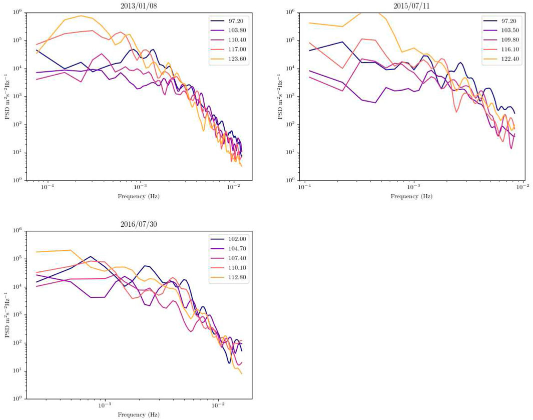
Figure 2. Frequency spectra for the measurements in shown in Figure 1 at various selected altitudes. The independent variable in these plots is frequency $f$ with units of cycles per second.

All of the spectra in Figure 2 obey a steep power low at frequencies greater than about $4\times 10^{-3}$ ${\text{s}}^{-1}$. This portion of the spectrum appears to be universal to the data and corresponds roughly to periods below the nominal buoyancy period. At longer periods, the spectra exhibit more variability and do not obviously follow power-low behavior. Most of the spectra exhibit a distinct peak, the frequency of the peak decreasing with increasing altitude and increasing wind fluctuation amplitude. This behavior is least apparent in the 2016 data corresponding to a structured sporadic E layer. In this case, the low-frequency portion of the spectra arguably follow a shallow power law spectral index close to $f^{-1}$. It is possible, however that the time series available from 2016 is merely insufficiently long to indicate clearly the outer scale of the flow.

Finally, Figure 3 shows the vertical wavenumber spectra for the three datasets calculated over a range of local times. Here, all the spectra appear to be rather similar, exhibiting almost universal behavior. As in the previous figure, the spectra follow power laws with relatively steep spectral indices at wavenumbers greater than about $5\times 10^{-1}$ ${\text{km}}^{-1}$ or vertical scale sizes smaller than about 2 km. At larger scales, the spectra arguably follow spectral indices close to $m^{-2}$. The data for 2016 have relatively little dynamic range in scale size and amplitude and so may not be especially informative other than being broadly consistent with the other datasets. In none of the three cases is it clear that the outer scale of the flow has been captured due to the relatively narrow altitude range over which wind estimation can be applied.

Figure 3

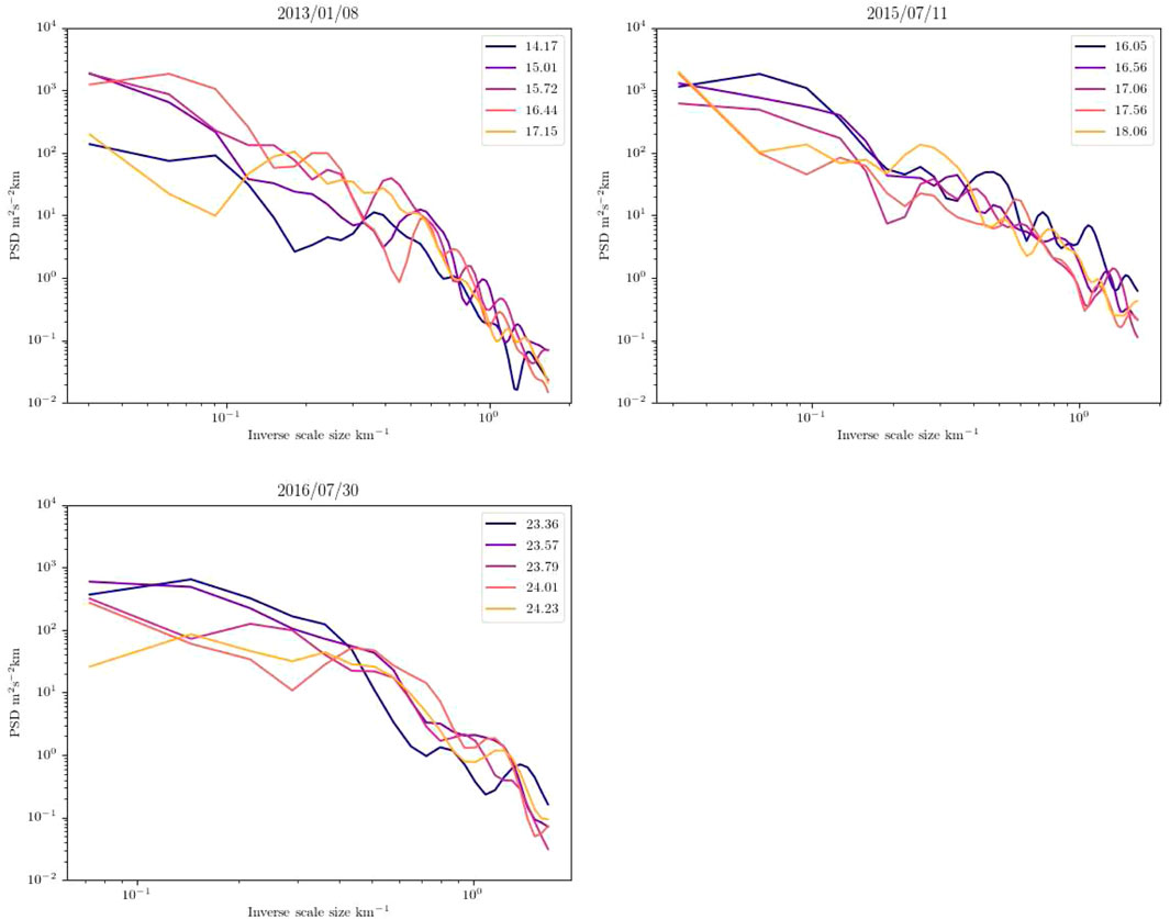
Figure 3. Vertical wavenumber spectra for the measurements in shown in Figure 1 at various selected local times. The independent variable in these figures is inverse scale size $m$ with units of cycles per kilometer.

4 Analysis

The Arecibo vertical wind data can be interpreted in view of other, similar datasets which have been summarized in the literature. While most of this work has concerned mesospheric winds, some comparisons remain possible. Vertical wind measurements from MST radars typically extend up through about only 95 km altitude where the wind speeds are generally limited to about $\pm$5 m/s and typically increasing with altitude, consistent with what is shown at the lowest altitudes represented in Figure 1 (e.g., Zhang et al., 2020). Wind profiles are most often presented in aggregate form, however, limiting comparisons with the individual datasets shown in Figure 1.

Interest has mainly focused on the frequency and wavenumber spectra of the vertical mesospheric winds and their averages since these can be tested against theory. Tsuda et al. (1990) presented vertical wind frequency spectra acquired in the mesosphere using the middle and upper (MU) VHF atmosphere radar in Japan. Their result exhibited a broad peak between about ${10}^{-4}$ and ${10}^{-3}$ c/s with a steep tail at higher frequencies that resembled some of the curves in Figure 2 albeit with a reduction in amplitude of about 10 dB.

Mitchell and Howells (1998) measured vertical wavenumber spectra of the vertical winds in the mesosphere with the EISCAT VHF radar over a year-long interval. For inverse scale sizes between ${10}^{-1}$ and ${10}^{-0.2}$ ${\text{km}}^{-1}$, they obtained (through regression) spectral indices for daily datasets ranging between $m^{-0.41}$ and $m^{-2.25}$. There was considerable scatter but also a clear seasonal dependence. This range of indices includes those measured with the EISCAT VHF radar in two short campaigns (Fritts and Hoppe, 1995) as well as with a sodium lidar in the altitude range between 84–100 km (Gardner et al., 1995), bridging the span to the Arecibo measurements to some degree. The lower-thermospheric vertical wind spectra from Arecibo are therefore similar to their mesospheric counterparts although both demonstrate considerable variability. All vertical wavenumber spectral estimates suffer from a limited vertical domain size, limiting the dynamic range of the spectrum and making it difficult to observe the outer scale of the flow.

The interpretation of the spectra is complicated, there being a number of candidate theoretical frameworks to consider (see, e.g., Gardner (1996); Fritts and Alexander (2003) for older reviews). While power-law spectra could be construed as evidence of stratified turbulence (e.g., Lilly, 1983), the actual power laws observed are not precisely what would be expected for turbulent cascades, and other frameworks have been proposed, especially frameworks based on saturated gravity wave theory in view of the characteristic increase of wind amplitudes and variances with altitude observed. Other frameworks emphasize the role of convective or dynamic instability (Dewan and Good, 1986; Smith et al., 1987) and buoyancy-range turbulence (Weinstock, 1985).

A large number of experiments and datasets have shown that the frequency spectra of horizontal winds (not considered in this paper) generally obey power laws at frequencies extending up to the buoyancy frequency, with spectral indices between −1 and −2 and possibly close to −5/3 being common (Fritts and Alexander, 2003). The frequency spectra of vertical velocities, meanwhile, exhibit more variability and altitude dependence. This is often interpreted as an effect of Doppler shifts which make relatively more important contributions to the measurements.

Vertical wavenumber spectra of horizontal and radial winds measured by a number of different instruments tend to exhibit broad peaks at large scales where energy is concentrated (tens of km in the mesosphere) and to decrease following power laws with decreasing scale size. A large number of studies have reported spectral indices in the range between −2.5 and −3 in the troposphere, stratosphere, and mesosphere, numbers which are broadly consistent with a body of gravity wave saturation theories as well as theories rooted in two-dimensional turbulence and in convective and dynamic instabilities (see Tsuda et al. (1989); Fritts and Alexander (2003) and references therein).

However, Mitchell and Howells (1998) reviewed the status of vertical wavenumber spectra of the vertical winds specifically. They pointed out that the observed spectral indices (mainly between −0.4 and −1.6) were consistent neither with the positive slopes predicted by gravity wave saturation theory nor the steep negative slopes predicted by linear instability theory. They pointed out that the presence of ducted gravity waves in the data may be contaminating the spectral results. The limited span of altitudes available for analysis also limits the experimental ability to observe the outer scale of the flow.

More recently Avsarkisov et al. (2022); Avsarkisov and Conte (2023) have offered a more comprehensive model of the turbulent processes in the atmosphere, including the mesosphere, across a broad range of spatial scales. Their article presents an extensive literature review of related work based on theory, modeling, and observations. Their results are based on analysis of the various theories, as well as calculations with a gravity-wave resolving numerical model and appear to be consistent with other modeling results and data analysis from studies that have addressed more narrow parts of the atmospheric spectrum or have addressed the physics from a specific focused perspective. Direct comparison with their predictions is not possible for our data since their analysis did not include specific predictions of the spectral indices for the vertical velocities. The spectral slopes presented here, as well as those shown by Mitchell and Howells (1998), deviate from the slopes found in studies based on measurements from the mesosphere which generally have steeper slopes. Complicating factors may include the change in dynamics across the turbopause transition.

5 Summary

This paper reviewed unique radar observations of the lower thermosphere acquired with the Arecibo Radio Observatory and the methods used to reduce them to vertical wind profile measurements. The winds are characterized by large amplitudes and variances, tendencies for sustained downdratfs, and considerable variability. The frequency spectra of the vertical winds exhibit broad peaks at low frequencies, shallow power laws up to the nominal buoyancy frequency, and steep spectral tails at higher frequencies. The amplitude of the spectra and the period of the peaks increase markedly with altitude.

The vertical wavenumber spectra of the vertical winds, meanwhile, have a more universal quality. They exhibit power-law behavior, with spectral indices close to −2 for scale sizes longer than about 2 km and somewhat steeper spectral indices at smaller scales. All together, the spectral characteristics of the lower thermospheric measurements are consistent with what has been observed by MST radars in the mesosphere.

Notable features in the data are the existence of a transition height where the vertical velocity magnitudes increase rapidly with height and the extended periods of sustained vertical winds in one direction. It is not clear what the drivers are for either of those features.

Until recently there did not appear to be a single theoretical framework capable of accounting for the measurements presented and reviewed here. The theories presented in the literature relied either on primarily vortical motion associated with stratified turbulence and inverse energy cascades, or on weakly interacting spectra of gravity waves representing a buoyancy subrange. The model presented by Avsarkisov et al. (2022); Avsarkisov and Conte (2023) bridges the various interpretations and argues for transitions from strongly rotational stratified turbulence at larger scales to stratified turbulence at intermediate scales to Kolmogoroff-type three-dimensional turbulence at smaller scales. Their article did not specifically predict spectral indices for the frequency and vertical wavelength spectra of the vertical velocity, so a direct comparison is not possible. Reproducing the radar measurements may necessitate direct numerical simulation of the dynamics of the mesosphere and lower thermosphere, a proposition that may finally be computationally tractable. 1n particular, the changes in spectral shapes and characteristic length and time scales across the turbopause boundary is of primary interest. The Arecibo data may, at least in part, provide some guidance and validation for such studies.

The Arecibo measurements were only possible because of the sensitivity of the instrument. Vertical-wind measurements only became practical in the last decade of operations due mainly to several innovations in incoherent scatter techniques involving pulse compression and frequency diversity. While Arecibo’s sensitivity is likely to remain unsurpassed for the immediate future, multistatic incoherent scatter radars that are emerging now, in development, or in planning stages should be able to infer neutral winds in the lower thermosphere with comparable or superior fidelity in view of the ambiguity that multistatic radar measurements can help resolve.

Data availability statement

The raw data supporting the conclusions of this article will be made available by the authors, without undue reservation.

Author contributions

DH: Conceptualization, Data curation, Funding acquisition, Investigation, Methodology, Project administration, Software, Visualization, Writing – original draft, Writing – review and editing. ML: Conceptualization, Formal Analysis, Funding acquisition, Investigation, Project administration, Writing – review and editing.

Funding

The author(s) declare that financial support was received for the research and/or publication of this article. The work was supported by NSF awards AGS-2011304 and AGS-2213849 to Cornell University and AGS-2012994 to Clemson University.

Conflict of interest

The authors declare that the research was conducted in the absence of any commercial or financial relationships that could be construed as a potential conflict of interest.

Generative AI statement

The author(s) declare that no Generative AI was used in the creation of this manuscript.

Any alternative text (alt text) provided alongside figures in this article has been generated by Frontiers with the support of artificial intelligence and reasonable efforts have been made to ensure accuracy, including review by the authors wherever possible. If you identify any issues, please contact us.

Publisher’s note

All claims expressed in this article are solely those of the authors and do not necessarily represent those of their affiliated organizations, or those of the publisher, the editors and the reviewers. Any product that may be evaluated in this article, or claim that may be made by its manufacturer, is not guaranteed or endorsed by the publisher.

References

Aster, R. C., Borchers, B., and Thurber, C. H. (2005). Parameter estimation and inverse problems. New York: Elsevier.

Google Scholar

Avsarkisov, V., and Conte, J. F. (2023). The role of stratified turbulence in the cold summer mesopause region. J. Geophys. Res. Atmos. 128, e2022JD038322. doi:10.1029/2022JD038322

CrossRef Full Text | Google Scholar

Avsarkisov, V., Becker, E., and Renkwitz, T. (2022). Turbulent parameters in the middle atmosphere: theoretical estimates deduced from a gravity wave–resolving general circulation model. J. Atmos. Sci. 79, 933–952. doi:10.1175/JAS–D–21–0005.1

CrossRef Full Text | Google Scholar

Bakhmetieva, N. V., and Zhemyakov, I. N. (2022). Vertical plasma motions in the dynamics of the mesosphere and lower thermosphere of the Earth. Russ. J. Phys. Chem. B16, 990–1007. doi:10.1134/S1990793122050177

CrossRef Full Text | Google Scholar

Behnke, R. A., and Kohl, H. (1974). The effects of neutral winds and electric fields on the ionospheric F2-layer over Arecibo. J. Atmos. Terr. Phys. 36, 325–333. doi:10.1016/0021-9169(74)90051-8

CrossRef Full Text | Google Scholar

Campbell, D. (2024). The Arecibo observatory: a history of innovation and discovery. Nature Switzerland AG: Springer.

Google Scholar

Dewan, E. M., and Good, R. E. (1986). Saturation and the “universal” spectrum for vertical profiles of horizontal scalar winds in the atmosphere. J. Geophys. Res. 91, 2742–2748. doi:10.1029/jd091id02p02742

CrossRef Full Text | Google Scholar

Emmert, J. T., Drob, D. P., Picone, J. M., Siskind, D. E., Jones, Jr., M., Mlynczak, M. G., et al. (2021). NRLMSIS 2.0: a whole-atmosphere empirical model of temperature and neutral species densities. Earth Space Sci. 8, e2020EA001321. doi:10.1029/.2020EA001321

CrossRef Full Text | Google Scholar

Fritts, D. C., and Alexander, M. J. (2003). Gravity wave dynamics and effects in the middle atmosphere. Rev. Geophys. 41. doi:10.1029/2001RG000106

CrossRef Full Text | Google Scholar

Fritts, D. C., and Hoppe, U. P. (1995). High-resolution measurements of vertical velocity with the European incoherent scatter VHF radar 2. Spectral observations and model comparisons. J. Geophys. Res. 100 (16), 16827–16838. doi:10.1029/95jd01467

CrossRef Full Text | Google Scholar

Gardner, C. S. (1996). Testing theories of atmospheric gravity-wave saturation and dissipation. J. Atmos. Sol. Terr. Phys. 58, 1575–1589. doi:10.1016/0021-9169(96)00027-x

CrossRef Full Text | Google Scholar

Gardner, C. S., Tao, X., and Papan, G. C. (1995). Simultaneous lidar observations of vertical wind, temperature and density profiles in the upper mesosphere: evidence for nonseperability of atmospheric perturbation spectra. Geophys. Res. Lett. 22, 2877–2880. doi:10.1029/94JD02748

CrossRef Full Text | Google Scholar

Harper, R. M. (1977). Tidal winds in the 100- to 200-km region at Arecibo. J. Geophys. Res. 82, 3243–3250. doi:10.1029/ja082i022p03243

CrossRef Full Text | Google Scholar

Harper, R. M., Wand, R. H., Zamlutti, C. J., and Farley, D. T. (1976). E region ion drifts and winds from incoherent scatter measurements at Arecibo. J. Geophys. Res. 81, 25–35. doi:10.1029/ja081i001p00025

CrossRef Full Text | Google Scholar

Hysell, D. L., Larsen, M. F., and Sulzer, M. P. (2014). High time and height resolution neutral wind profile measurements across the mesosphere/lower thermosphere region using the Arecibo incoherent scatter radar. J. Geophys. Res. 119, 2345–2358. doi:10.1002/2013JA019621

CrossRef Full Text | Google Scholar

Hysell, D., Larsen, M., and Sulzer, M. (2016). Observational evidence for new instabilities in the midlatitude E and F region. Ann. Geophys. 34, 927–941. doi:10.5194/angeo-34-927-2016

CrossRef Full Text | Google Scholar

Hysell, D. L., Larsen, M. F., Fritts, D. C., Laughman, B., and Sulzer, M. P. (2018). Major upwelling and overturning in the mid-latitude F region ionosphere. Nat. Comm. 9, 3326. doi:10.1038/s41467–018–05809–x

PubMed Abstract | CrossRef Full Text | Google Scholar

Larsen, M. F., and Meriwether, J. W. (2012). Vertical winds in the thermosphere. J. Geophys. Res. 117. doi:10.1029/2012JA017843

CrossRef Full Text | Google Scholar

Lilly, D. K. (1983). Stratified turbulence and the mesoscale variability of the atmosphere. J. Atmos. Sci. 40, 749–761. doi:10.1175/1520-0469(1983)040<0749:statmv>2.0.co;2

CrossRef Full Text | Google Scholar

Mitchell, N. J., and Howells, V. S. C. (1998). Vertical velocities associated with gravity waves measured in the mesosphere and lower thermosphere with the EISCAT VHF radar. Ann. Geophys. 16, 1367–1379. doi:10.1007/s00585-998-1367-0

CrossRef Full Text | Google Scholar

Nygrén, T., Aikio, A. T., Kuula, R., and Voiculescu, M. (2011). Electric fields and neutral winds from monostatic incoherent scatter measurements by means of stochastic inversion. J. Geophys. Res. 116. doi:10.1029/2010JA016347

CrossRef Full Text | Google Scholar

Richards, P. G., Bilitza, D., and Voglozin, D. (2010). Ion density calculator (IDC): a new efficient model of ionospheric ion densities. Radio Sci. 45. doi:10.1029/2009RS004332

CrossRef Full Text | Google Scholar

Schunk, R. W., and Nagy, A. F. (2004). Ionospheres: physics, plasma physics, and chemistry. Cambridge, United Kingdom: Cambridge Univ. Press.

Google Scholar

Smith, S. A., Fritts, D. C., and VanZandt, T. E. (1987). Evidence for a saturated spectrum of atmospheric gravity waves. J. Atmos. Sci. 44, 1404–1410. doi:10.1175/1520-0469(1987)044<1404:efasso>2.0.co;2

CrossRef Full Text | Google Scholar

Sulzer, M. P. (1986a). A phase modulation technique for a sevenfold statistical improvement in incoherent scatter data-taking. Radio Sci. 21, 737–744. doi:10.1029/rs021i004p00737

CrossRef Full Text | Google Scholar

Sulzer, M. P. (1986b). A radar technique for high range resolution incoherent scatter autocorrelation function measurements utilizing the full average power of klystron radars. Radio Sci. 21, 1033–1040. doi:10.1029/rs021i006p01033

CrossRef Full Text | Google Scholar

Sulzer, M. P., Aponte, N., and González, S. A. (2005). Application of linear regularization methods to Arecibo vector velocities. J. Geophys. Res. 110 (A10). doi:10.1029/2005JA011042

CrossRef Full Text | Google Scholar

Thébault, E., Finlay, C., Beggan, C., Alken, P., Aubert, J., Barrios, O., et al. (2015). International geomagnetic reference field: the 12th generation. Earth, Plantes, Space 67, 79. doi:10.1186/s40623–015–0228–9

CrossRef Full Text | Google Scholar

Tsuda, T., Inoue, T., Fritts, D. C., Van Zandt, T. E., Kato, S., Sato, T., et al. (1989). MST radar observations of a saturated gravity wave spectrum. J. Atmos. Sci. 46, 2440–2447. doi:10.1175/1520-0469(1989)046<2440:mrooas>2.0.co;2

CrossRef Full Text | Google Scholar

Tsuda, T., Kato, S., Yokoi, T., Inoue, T., Yamamoto, M., VanZandt, T. E., et al. (1990). Gravity waves in the mesosphere observed with the middle and upper atmosphere radar. Radio Sci. 26, 1005–1018. doi:10.1029/rs025i005p01005

CrossRef Full Text | Google Scholar

Vasseur, G. (1969). Vents dans la thermosphere déduits des mesures par diffusion de Thomson. Ann. Geophys. 25, 517–527.

Google Scholar

Weinstock, J. (1985). Theoretical gravity wave spectrum in the atmosphere: strong and weak wave interactions. Radio Sci. 20, 1295–1300. doi:10.1029/rs020i006p01295

CrossRef Full Text | Google Scholar

Woodman, R. F., and Guillén, A. (1974). Radar observations of winds and turbulence in the stratosphere and mesosphere. J. Atmos. Sci. 31, 493–505. doi:10.1175/1520-0469(1974)031<0493:roowat>2.0.co;2

CrossRef Full Text | Google Scholar

Zhang, W., Chen, G., Zhang, S., Gong, W., Chen, F., He, Z., et al. (2020). Statistical study of the midlatitude mesospheric vertical winds observed by the Wuhan and Beijing MST radars in China. J. Geophys. Res. 125, e2020JD032776. doi:10.1029/2020JD032776

CrossRef Full Text | Google Scholar