 Huayu Zhao
 Huigen Yang
 Zejun Hu
 Dehong Huang2
 Jianjun Liu
- 1Shandong Key Laboratory of Optical Astronomy and Solar-Terrestrial Environment, School of Space Science and Technology, Institute of Space Sciences, Shandong University, Weihai, Shandong, China
- 2MNR Key Laboratory for Polar Science, Polar Research Institute of China, Shanghai, China
In this work, we present two individual cases showing that a negative solar wind dynamic pressure pulse can lead to magnetospheric decompression and generate a clockwise vortex in the duskside magnetosphere. In response to this decompression, a magnetospheric vortex in the duskside sector was observed by the Time History of Events and Macroscale Interactions during Substorms (THEMIS) mission. Minimum variance analysis (MVA) of the mass flux, together with the corresponding equivalent ionospheric currents (EICs), indicates that the magnetospheric vortex rotated clockwise which is opposite to the typical direction of vortices induced by positive solar wind dynamic pressure pulses. The associated clockwise EICs vortex suggests that the magnetospheric vortex was connected to the ionospheric vortex via downward field-aligned currents (FACs). Time series analysis of the EICs further reveals that the vortex propagated eastward, consistent with the tailward motion of the magnetospheric vortex. Moreover, the occurrence of the clockwise EIC vortex at lower latitudes, together with the THEMIS satellite location, indicates that the magnetospheric vortices associated with traveling convection vortices (TCVs) are generated not at the magnetopause, but within the nightside magnetosphere.
1 Introduction
Sudden changes in solar wind dynamic pressure can greatly influence the magnetosphere–ionosphere coupling system. It has long been known that the shape of the magnetosphere can be controlled by solar wind dynamic pressure and that the magnetosphere can be compressed by a positive dynamic pressure pulse. Furthermore, such positive pulses can generate numerous geo-effects within the magnetosphere–ionosphere coupling system. For example, observations from global magnetometer arrays indicate that a positive dynamic pressure pulse can lead to geomagnetic sudden impulses (SI+) (e.g., Araki, 1994). Positive dynamic pressure pulses have also been shown to play an important role in generating ultra-low frequency (ULF) waves (e.g., Kaufmann and Walker, 1974; Nopper et al., 1982; Wedeken et al., 1984; Cahill et al., 1990; Sarris et al., 2010; Shi et al., 2013). Zhao et al. (2019) found that such solar wind dynamic pressure pulses can directly excite field line resonances (FLRs) by using multipoint observation from THEMIS satellites, and they also provide the distribution of the FACs associated with FLRs in the same longitude but different latitudes. At lower altitudes, positive dynamic pressure pulses can induce traveling convection vortices (TCVs), as observed using incoherent scatter radars (Lühr et al., 1996; Valladares et al., 1999) and Super Dual Auroral Radar Network (SuperDARN) radars (Kataoka et al., 2003; Lyatsky et al., 1999). These TCVs are not static but propagate from the dayside to the nightside at speeds of several kilometers per second, consistent with the dynamic pressure pulse sweeping across the magnetosphere from the dayside to the magnetotail (e.g., Friis-Christensen et al., 1988; Glassmeier et al., 1989; Glassmeier et al., 1992; Kivelson and Southwood, 1991; Lühr et al., 1996; Yahnin and Moretto, 1996). At even lower altitudes, positive dynamic pressure pulses play an important role in modulating auroral phenomena, with auroral intensification typically starting near local noon and then extending toward the nightside along the dawn and dusk flanks of the auroral oval (e.g., Meurant et al., 2003; Zhou and Tsurutani, 1999; Zhou et al., 2003).
In contrast to the extensive studies on the geo-effects of positive dynamic pressure pulses, studies on the response of the magnetosphere–ionosphere coupling system to negative dynamic pressure pulses are relatively scarce (e.g., Akasofu, 1964; Araki and Nagano, 1988; Takeuchi et al., 2002). As a mirror response to the positive pulse, Araki and Nagano (1988) proposed that ground magnetic variations induced by negative dynamic pressure pulses oscillate in the opposite direction to those caused by positive pulses. Zhang et al. (2010) found that negative dynamic pressure pulses can also generate ULF waves, though the amplitudes are smaller than those associated with positive pulses. Negative pulses also play a role in generating TCVs, and Motoba et al. (2003) reported that negative pulses can induce clockwise ionospheric vortices on the duskside. Hori et al. (2012) found that evening-sector TCVs propagate poleward, consistent with negative pressure pulses sweeping the magnetosphere from the dayside to the nightside. Furthermore, Zhao et al. (2016) reported that such pulses can generate counterclockwise magnetospheric vortices on the dawnside; however, their study did not present observational or simulation results for the duskside magnetosphere.
Sibeck (1990) proposed a model illustrating the magnetospheric perturbation response to positive dynamic pressure pulses, in which magnetospheric vortices form near the dawn and dusk flanks. Shi et al. (2014) further suggested that such positive pulses can generate both clockwise and counterclockwise rotating vortices in the dawnside and duskside magnetosphere, respectively. Later, Shi et al. (2020) modified the model, proposing that negative pressure pulses can also generate vortices near the dawn and dusk flanks, but with opposite rotation directions compared to those induced by positive pulses. However, global MHD simulations by Yu and Ridley (2009) suggest that the FACs on the duskside flanks are not consistent with the Sibeck and Shi models. Specifically, the simulations show clear upward downward FACs on the duskside magnetosphere after a positive pulse. Notably, Yu and Ridley (2009) did not include any in situ observational verification, and no published studies have focused specifically on the duskside response to negative dynamic pressure pulses. Therefore, it is important to obtain in situ observations of magnetospheric vortices in the duskside magnetosphere following negative dynamic pressure pulses. Furthermore, Araki (1994) proposed that magnetospheric vortices can drive ionospheric vortices via FACs, and that these ionospheric vortices should propagate in tandem with their magnetospheric counterparts. However, no study has yet confirmed this relationship for negative dynamic pressure pulses. Thus, it remains unclear whether such pulses can generate both magnetospheric and ionospheric vortices on the duskside magnetosphere, and whether the two structures co-propagate.
In this study, we report the first direct, chain-type observation of a clockwise magnetospheric vortex and a corresponding equivalent ionospheric currents (EICs) vortex associated with a negative solar wind dynamic pressure pulse in the duskside sector. The dataset is presented in Section 2, and observations are described in Section 3. The discussion and conclusions are provided in Sections 4 and 5.
2 Materials and methods
In order to correlate negative solar wind dynamic pressure pulses with magnetospheric vortices in the duskside magnetosphere, observations of solar wind and interplanetary magnetic field (IMF) parameters from the WIND spacecraft are used in this study (e.g., Farrell et al., 1995; Gloeckler et al., 1995). In addition, the solar wind dynamic pressure and SYM-H index obtained from the OMNI database are also used. The THEMIS mission provides observations of magnetospheric vortices following negative solar wind dynamic pressure pulses. The electrostatic analyzer onboard THEMIS provides magnetospheric plasma parameters (McFadden et al., 2008), while the fluxgate magnetometer measures the three components of the magnetic field (Auster et al., 2008). The time series of EICs are calculated using the spherical elementary current system (SECS) method, based on data from AUTUMN, MACCS, STEP, McMAC, CANMOS, USGS, CARISMA, and ground magnetometers operated by DTU.
3 Results
3.1 Event on 09 March 2017
On 09 March 2017, the WIND satellite detected a negative solar wind dynamic pressure pulse (from 1.6 nPa to 1.0 nPa) at 02:27:30 UT, as shown in Figure 1a. All three components of the solar wind velocity showed slight decreases when the pressure drop occurred, and the solar wind density clearly decreased from 3.3 cm−3 to 2.3 cm−3 (Figures 1b,c). These results indicate that the negative dynamic pressure pulse was primarily caused by a drop in solar wind density. Figure 1d presents the three components of the IMF in GSM coordinates: the x-component remained positive, while the y- and z-components stayed negative. The dashed line marks the negative dynamic pressure pulse. The propagation time from the WIND satellite to the magnetosphere is calculated to be 3,390 s, based on the satellite’s position and the solar wind velocity. Accordingly, the arrival of the negative dynamic pressure pulse at the magnetosphere was at 03:25 UT, as shown in Figure 1e. Figure 1f shows the SYM-H index from the OMNI database, where a decrease following the dashed line indicates magnetospheric decompression caused by the pressure drop.
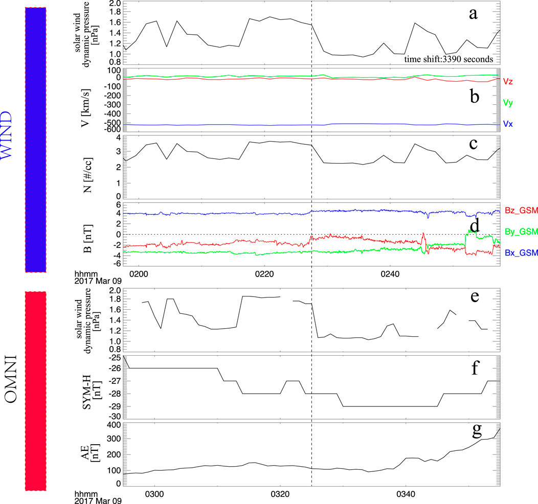
Figure 1. Wind observations of solar wind and IMF parameters on 9 March 2017, shown in the upper panel. The solar wind dynamic pressure and SYM-H index are derived from the OMNI database. (a) Solar wind dynamic pressure. (b) Three components of solar wind velocity in GSM coordinates. (c) Solar wind density. (d) X, Y, and Z components of the IMF. (e) solar wind dynamic pressure derived from OMNI data base (f) SYM-H index. (g) AE index.
After the magnetosphere was decompressed by the negative dynamic pressure pulse, the THEMIS-E satellite has observed the corresponding magnetospheric perturbations between 03:25 UT and 03:35 UT in the duskside magnetosphere, as shown in Figure 2. Before the pulse impacted the magnetosphere, no significant plasma flow velocity oscillations were recorded. Upon the arrival of the pulse, clear bipolar oscillations in the plasma flow velocity were observed. After 03:35 UT, the amplitude of these oscillations increased significantly, which is attributed to a subsequent positive solar wind dynamic pressure pulse occurring at that time. Therefore, the post-03:35 UT interval is excluded from our analysis, as our focus is solely on the geo-effects associated with the negative pressure pulse. The x and y components of the magnetospheric plasma flow velocity exhibited distinct bipolar signatures following the pulse, indicating that the perturbations were primarily confined to the x–y plane. The three components of the magnetic field also showed clear perturbations in response to the pulse (Figures 2c,d). The electron and ion observations exhibit a clear decrease following the arrival of the negative solar wind dynamic pressure pulse at the magnetosphere, indicating that the magnetosphere underwent a decompression process, as shown in Figures 2e,f. According to Keiling et al. (2009), such bipolar velocity signatures may indicate the passage of a satellite through a plasma flow vortex. To confirm the presence of a vortex, we applied the MVA method on the mass flux (e.g., Sonnerup and Scheible, 1998; Zong et al., 2009), and transformed the data into the MVA coordinate system (Figure 3). Figure 3a shows the results of MVA method in the maximum (ρVl) and intermediate (ρVm) variance directions, while Figure 3b shows the results in the maximum and minimum (ρVn) variance directions. The large-scale rotational pattern observed in Figure 3a confirms that the bipolar velocity signature corresponds to a plasma flow vortex. Furthermore, the red “s” and blue “e” markers indicate the start and end points of the trajectory, respectively, showing that the rotation is clockwise.
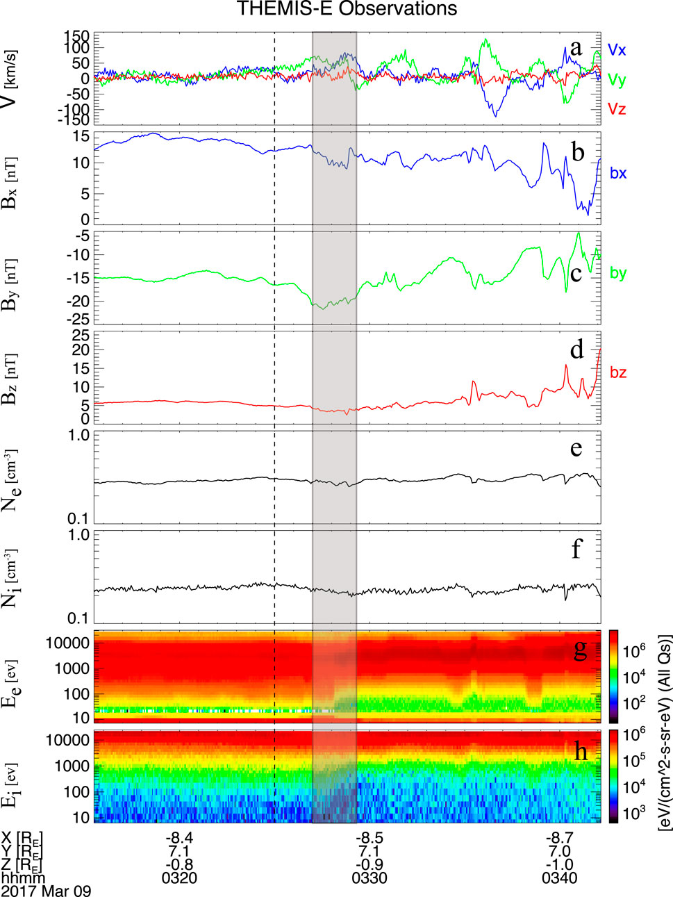
Figure 2. Magnetospheric observations from the THEMIS-E satellite in the duskside magnetosphere following a negative solar wind dynamic pressure pulse. (a) Three components of magnetospheric plasma flow velocity. (b–d) X, Y, and Z components of the magnetic field in GSM coordinates. (e), (f) Temporal variations of electron and ion density. (g), (h) Electron and ion energy flux. The shaded area represents the bipolar signature of plasma flow velocity, which corresponds to the magnetospheric vortex.
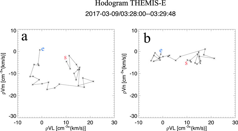
Figure 3. Hodograms derived using the MVA (Minimum Variance Analysis) method on the mass flux of the magnetospheric vortex. (a) ρVl and ρVm represent the components along the maximum and intermediate variance directions in the MVA coordinate system. (b) ρVl and ρVn show the components along the maximum and minimum variance directions. The red “s” and blue “e” indicate the start and end points of the flow, respectively.
Araki (1994) first proposed that magnetospheric vortices generated by positive dynamic pressure pulses could correlate with corresponding ionospheric vortices via FACs near the footpoint of the vortex. To investigate whether a magnetospheric vortex induced by a negative dynamic pressure pulse also corresponds to an ionospheric vortex in the duskside magnetosphere, we traced magnetic field lines from the THEMIS-E satellite to the ionosphere. Using the T96 magnetic field model with real-time solar wind and IMF parameters, we determined the footpoint of the THEMIS-E satellite in the northern hemisphere, as shown in Figure 4. The blue dot marks the footpoint, and the map includes the altitude-adjusted corrected geomagnetic (AACGM) coordinate grid. The footpoint is located over North America, allowing us to use data from North American ground magnetometers to analyze ionospheric responses. To derive the EICs, we applied the spherical elementary current system method using ground magnetometer data (e.g., Amm and Viljanen, 1999; Weygand et al., 2011). Figure 5 presents the EICs in the northern hemisphere from 03:24 UT to 03:35 UT. The THEMIS-E footpoint is again marked by a blue dot. Before the negative pressure pulse impacted the magnetosphere, EICs showed a stripe pattern oriented from the west-north toward the east-south direction—this pattern is unrelated to the pressure pulse. At 03:27 UT, no clear vortex structure was present near the satellite footpoint. However, beginning at 03:27 UT, the EICs intensified and a clockwise ionospheric vortex started to form, becoming clearly visible by 03:28 UT. The time series EICs results reveal that the EICs vortex propagates from westside to eastside, which is consistent with the tailward moving magnetospheric vortex.
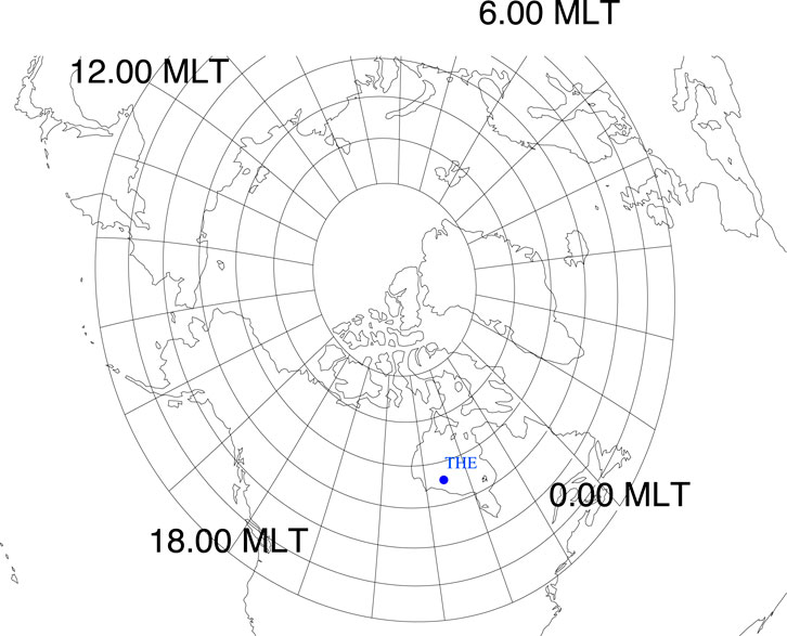
Figure 4. Magnetic local time grid and the footpoint of the THEMIS-E satellite in the Northern Hemisphere, shown in altitude-adjusted corrected geomagnetic coordinates (AACGM). The blue solid dot indicates the location of the THEMIS-E satellite footpoint.
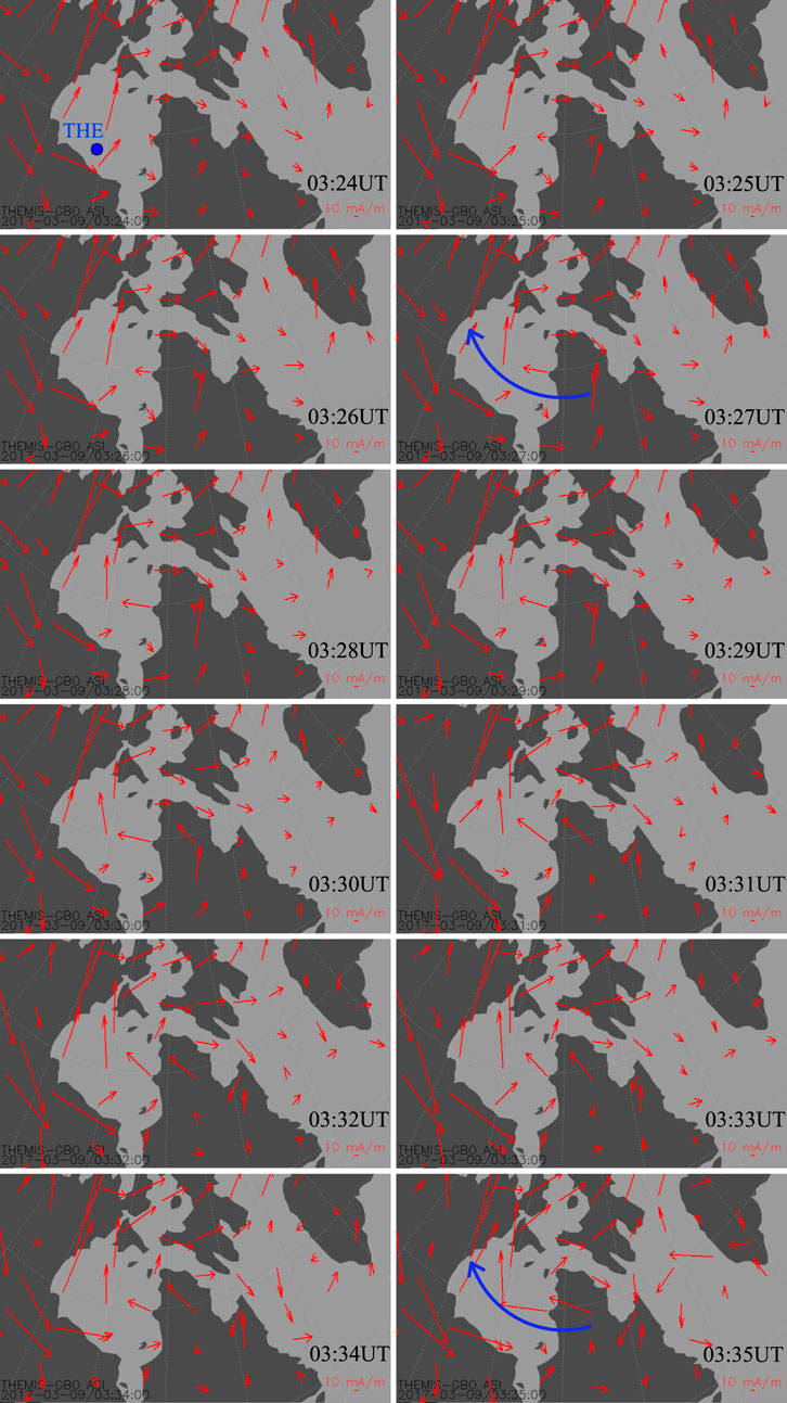
Figure 5. Equivalent ionospheric currents (EICs) near the footpoint of the satellite in the Northern Hemisphere from 03:24 UT to 03:35 UT. Red arrows indicate ionospheric current vectors. The footpoint of the THEMIS-E satellite is marked by a solid blue dot in the first panel. The solid blue arrow denotes the clockwise rotation of the EIC vectors.
3.2 Event on 3 January 2015
On 3 January 2015, the WIND satellite detected a distinct negative solar wind dynamic pressure pulse (from about 9.2 nPa to 4 nPa), as shown in Figure 6a. The WIND observations further indicate that this negative pressure pulse was mainly caused by a decrease in solar wind density, while the solar wind velocity also showed a slight decrease (Figures 6b,c). Based on the solar wind velocity and the WIND satellite’s position, a time shift of about 2,610 s was calculated. Subsequently, the SYM-H index recorded a decrease from about −15 nT to −30 nT, indicating that the magnetosphere underwent decompression.
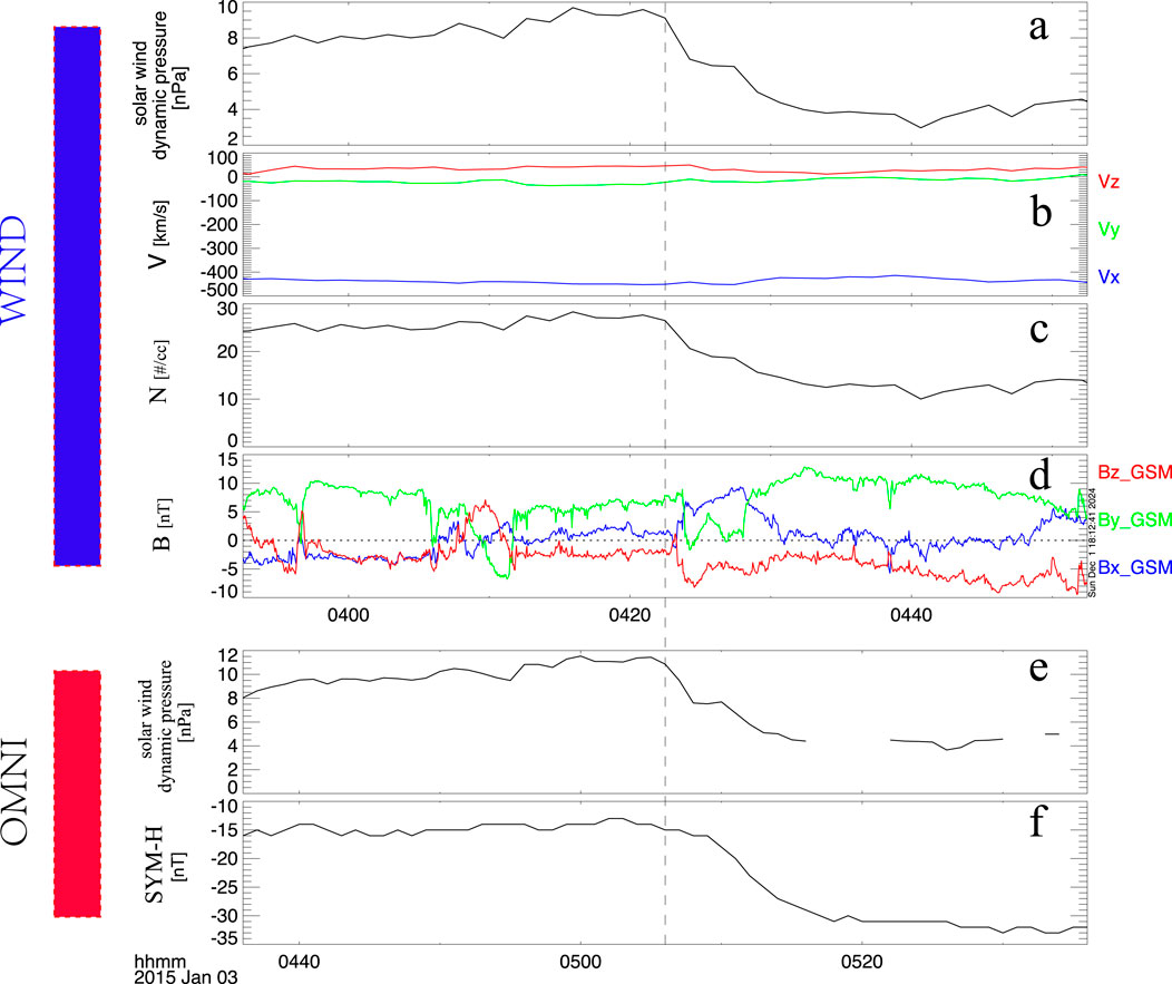
Figure 6. Solar wind parameters and IMF derived from the WIND satellite and OMNI database on 3 January 2015. (a) Solar wind dynamic pressure. (b) Three components of solar wind velocity in GSM coordinates. (c) Solar wind density. (d) Three components of the IMF. (e) Solar wind dynamic pressure from the OMNI database. (f) SYM-H index from the OMNI database. The dashed line indicates the onset time of the negative solar wind dynamic pressure pulse.
Figure 7 presents three THEMIS satellites observations of magnetospheric perturbations after the negative solar wind dynamic pressure pulse reached the magnetosphere. The dashed line corresponds to the initial onset time of the pressure decrease, consistent with the timing in Figure 6. After the pressure pulse arrived at the magnetosphere, the three THEMIS satellites (THEMIS-A, D, and E) observed a clear bipolar signature in magnetospheric plasma flow velocity (Figures 7a,h,o), indicating that the perturbations in plasma flow velocity were associated with a magnetospheric flow vortex (e.g., Keiling et al., 2009). The total magnetic field shows a clear decrease after the negative solar wind dynamic pressure pulse arrives at the magnetosphere (Figures 7b,i,p), indicating that the magnetosphere underwent decompression. This decompression is also evidenced by the decrease in ion density following the pulse (Figures 7e,l,s). Figures 7g,h show the positions of the three THEMIS satellites in the XY and YZ planes. All three satellites observed similar magnetospheric perturbations but at different times: THEMIS-D, located closest to Earth, observed them first; THEMIS-E, located in between, observed them next; and THEMIS-A, positioned farther in the magnetotail, observed them last. This time sequence, also evident in Figure 7, suggests that the magnetospheric perturbations induced by the negative solar wind dynamic pressure pulse propagated tailward.
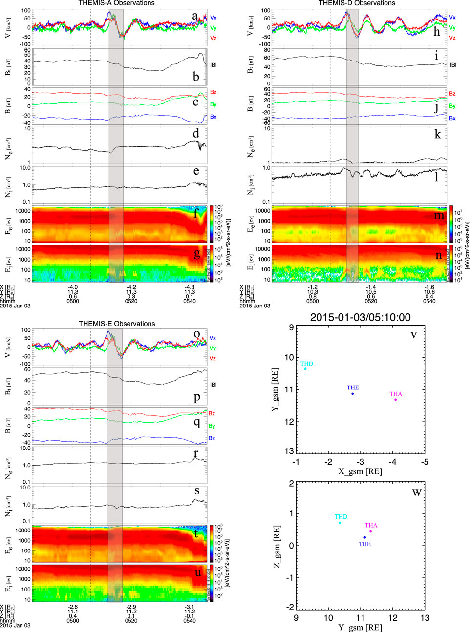
Figure 7. Magnetospheric observations from three THEMIS satellites and their positions in the xy and yz planes. The dashed line marks the onset time of the negative solar wind dynamic pressure pulse, identical to that in Figure 6. The shaded area highlights the bipolar plasma flow velocity signature corresponding to the magnetospheric vortex. (a,h,o) Three components of magnetospheric plasma flow velocity observed by THEMIS-A, -D, and -E, respectively. (b,i,p) Total magnetic field measured by the three THEMIS satellites. (c,j,q) Three components of the magnetic field from the three THEMIS satellites. (d,k,r) Electron density. (e,l,s) Ion density. (f,m,t) Electron energy flux. (g,n,u) Ion energy flux. (v,w) Positions of the three THEMIS satellites in the xy and yz planes, respectively.
Figure 8 shows the EIC results near the footpoints of the three THEMIS satellites in the Northern Hemisphere from 05:14 UT to 05:17 UT. The footpoints were derived from the T96 model using realistic solar wind and IMF parameters. In the 05:14 UT image (Figure 8), the three THEMIS footpoints are represented by solid dots. Before 05:14 UT, no EIC vortex was observed near the footpoints of the THEMIS satellites. At 05:15 UT, however, a clear clockwise EIC vortex appeared near the satellite footpoints. By 05:16 UT, this clockwise EIC had propagated eastward, consistent with the tailward-propagating magnetospheric vortex.
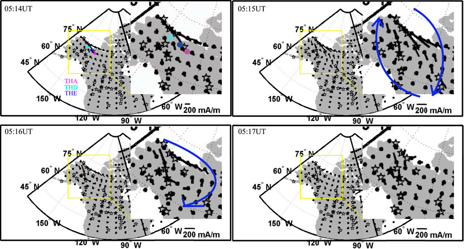
Figure 8. EICs observed near the northern hemisphere footpoints of the THEMIS satellites from 05:14 UT to 05:17 UT. The solid red, light blue, and blue dots represent the footpoints of THEMIS-A, THEMIS-D, and THEMIS-E, respectively. The yellow rectangle indicates a region of interest, which is enlarged in the upper-right corner of each panel. The solid blue circular vector denotes the rotated EIC vortex and its rotation direction.
4 Discussion
In this work, we presented two individual cases demonstrating that negative solar wind dynamic pressure pulses can drive magnetospheric decompression and generate clockwise vortices in the duskside magnetosphere. The associated EICs further suggest a coupling through downward FACs, with the vortex propagating eastward in agreement with the tailward motion of the magnetospheric vortex. Moreover, the occurrence of the clockwise EIC vortex at lower latitudes, together with the satellite location, implies that the FACs linked to TCVs were generated within the nightside magnetosphere rather than at the magnetopause.
In this work, we present two individual cases showing that solar wind dynamic pressure pulses can generate clockwise magnetospheric vortices in the duskside magnetosphere. In the first case, the solar wind dynamic pressure decreased from 1.6 nPa to 1.0 nPa, while in the second case it decreased from about 9.2 nPa to 4 nPa. In both cases, the THEMIS satellites observed a clockwise magnetospheric vortex in the duskside magnetosphere. The first case involved only a small decrease of about 0.6 nPa, whereas the second case involved a much larger decrease of about 5.2 nPa. Nevertheless, both small- and large-scale negative dynamic pressure pulses were capable of generating clockwise vortices. It is well established that positive solar wind dynamic pressure pulses can induce magnetospheric vortices on both the dayside and duskside magnetosphere (e.g., Sibeck, 1990; Shi et al., 2014; Tian et al., 2016). The generation of such vortices is typically attributed to fast magnetosonic waves launched by the sudden compression of the magnetosphere (e.g., Samsonov and Sibeck., 2013; Shi et al., 2014). These waves propagate from the magnetopause toward the inner magnetosphere and then reflect at internal boundaries such as the plasmapause or ionosphere. The combined penetration and reflection of these waves subsequently form vortex-like flow patterns (e.g., Shi et al., 2014; Tian et al., 2016). For negative solar wind dynamic pressure pulses, we also adopt this explanation: the basic vortex structure can be induced by the generation and reflection of fast magnetosonic waves (e.g., Zhao et al., 2016). When a negative pressure pulse reaches the magnetosphere, it can excite a fast magnetosonic wave that propagates toward the magnetopause. Upon reaching the outer boundary, the fast mode wave is reflected at the magnetopause and then propagates earthward. Furthermore, the Ampère force at the front of the fast magnetosonic wave can accelerate plasma along the direction of wave propagation. As a result, the generation and reflection of fast mode waves form a basic plasma flow vortex, rotating in the opposite direction to that induced by positive solar wind dynamic pressure pulses (e.g., Zhao et al., 2016; Shi et al., 2020). In the first case, a solar wind dynamic pressure increase (from about 1.1 nPa to 1.6 nPa) was observed approximately 12 min before the negative solar wind dynamic pressure pulse. The negative pressure pulse occurred at around 03:13 UT, while the corresponding magnetospheric perturbations were detected by the THEMIS satellite at 03:25 UT. Furthermore, the expected sense of rotation of the magnetospheric vortex associated with a positive pressure impulse should be counterclockwise, which is opposite to the clockwise rotation of the magnetospheric vortex observed in this study. Therefore, we conclude that the magnetospheric perturbations detected by THEMIS were induced by the negative solar wind dynamic pressure pulse. Zhang et al. (2010) proposed a criterion that a solar wind dynamic pressure pulse can be identified when the variation of dynamic pressure exceeds either 1 nPa or 50%. Such pulses are considered capable of generating ultra-low-frequency waves inside the magnetosphere. In this work, the first event does not satisfy this criterion; however, the negative pulse still generated a magnetospheric vortex. We suggest that the requirement of a 50% variation may be too strict, and we plan to analyze more cases in a statistical study to determine a more appropriate threshold for whether a pulse can generate magnetospheric vortices.
Through the different amplitudes of solar wind dynamic pressure decreases, both cases in this work generate magnetospheric vortices, but the corresponding magnetospheric and ionospheric responses are very different. In the first case, the solar wind dynamic pressure decreased by only about 0.6 nPa, whereas in the second case it decreased by about 5.2 nPa. The amplitude of the magnetospheric plasma flow velocity perturbation is about 50 km/s in the first case, and about 100 km/s in the second case. Keiling et al. (2009) proposed that the magnitude of FACs is proportional to the speed of the rotating plasma flow vortex. This suggests that the FACs in the second case should be approximately twice those in the first case, assuming other parameters remain similar. In this study, we used the spherical elementary currents systems method to calculate EICs. If we assume a zero gradient of ionospheric conductance in the direction perpendicular to the electric field, the Hall-to-Pedersen conductance ratio becomes proportional to the FACs intensity (e.g., Amm and Kauristie, 2002; Weygand et al., 2011). Using this approach, we calculated the FACs induced by the negative solar wind dynamic pressure pulses. The downward FACs induced by the clockwise magnetospheric vortex are about −13,053 A for the first case, and about −25,984 A for the second case. These results are consistent with the theoretical framework proposed by Keiling et al. (2009), confirming that stronger plasma flow vortices produce stronger FACs. The FACs results show that while solar wind dynamic pressure pulses of different amplitudes can both generate magnetospheric vortices, but the resulting FAC intensities are very different. Furthermore, in both cases the SYM-H index lags behind the negative solar wind dynamic pressure pulse by several minutes. In the first case, the delay is about 5 min, while in the second case it is about 3 min. When the solar wind dynamic pressure decreases, the magnetopause expands outward, leading to a global reconfiguration of magnetospheric current systems. This process involves several stages. First, the pressure disturbance must be transmitted from the solar wind into the magnetosheath and then into the magnetosphere. Although fast-mode and Alfvén waves can propagate rapidly, the perturbation still requires a finite time (typically a few minutes) to reach the inner magnetosphere. Second, while the magnetopause and tail currents are modified almost immediately, the ring current and partial ring current respond more gradually, as their variations depend on the drift and redistribution of energetic ions in the equatorial plane. This inertia of the current systems delays the manifestation of the disturbance in ground-based indices. Third, the SYM-H index is derived from an average of multiple low-latitude magnetometer stations. Therefore, even if local perturbations appear promptly at some stations, the index only reflects the global change once the disturbance has developed coherently across a broad longitudinal extent. Taken together, the propagation of the pressure pulse, the dynamical adjustment of magnetospheric currents, and the averaging nature of SYM-H account for the observed several-minute delay.
According to Sibeck (1990), magnetospheric vortices driven by dynamic pressure variations propagate from the dayside toward the nightside along the magnetopause, implying that they are generated near the magnetopause. Araki (1994) further proposed that positive dynamic pressure pulses can simultaneously excite paired vortices in both the dawnside and duskside magnetosphere, each linked to corresponding ionospheric vortices via FACs. This model suggests a mirrored relationship between magnetospheric and ionospheric vortices, implying that ionospheric vortices should propagate in concert with their magnetospheric counterparts. Thus, if a magnetospheric vortex moves from the dayside to the nightside, the associated ionospheric vortex should exhibit a similar motion. In the second case, we present multi-satellite THEMIS observations of a magnetospheric vortex. A clear time lag is observed in the magnetospheric plasma flow velocity (Figure 7), allowing us to use multi-point measurements to calculate the vortex’s propagation speed. The estimated speed is about 297 km/s, which is smaller than the solar wind velocity of 460 km/s. The corresponding EICs vortex propagation speed is about 7.8 km/s, which corresponds to roughly 290 km/s at the magnetopause, similar to the magnetospheric vortex propagation speed. Furthermore, the propagation speed of the EICs vortex closely matches the shock aurora propagation speed of 6–11 km/s (e.g., Zhou et al., 2009). This similarity suggests a strong relationship between shock auroras and magnetospheric vortices following solar wind dynamic pressure pulses. Although no corresponding auroral observations are available for these cases, we plan to address this question in future studies by analyzing additional events.
5 Conclusion
In this work, we present a causal chain demonstrating that a negative solar wind dynamic pressure pulse can generate a clockwise magnetospheric vortex in the duskside magnetosphere. A corresponding clockwise EICs vortex can also be generated via downward FACs. The time series of the EICs results indicates that the EICs vortex propagated eastward, consistent with a tailward-moving magnetospheric vortex. Furthermore, the FACs associated with TCVs are located inside the magnetosphere rather than on the magnetopause in the nightside sector. In future studies, we will investigate more cases of magnetospheric and corresponding ionospheric vortices using in situ observations and global MHD simulations.
Data availability statement
The original contributions presented in the study are included in the article/supplementary material, further inquiries can be directed to the corresponding author.
Author contributions
HZ: Writing – original draft, Writing – review and editing. HY: Funding acquisition, Writing – review and editing. ZH: Writing – review and editing. DH: Writing – review and editing. BL: Writing – review and editing. BZ: Writing – review and editing. JL: Writing – review and editing.
Funding
The author(s) declare that financial support was received for the research and/or publication of this article. This research was funded by Natural Science Foundation of Shanghai, grant number 21DZ1206100 and by the National Natural Science Foundation of China (42130210).
Acknowledgments
We are very grateful to NASA THEMIS contract NAS5-02099; J. Bonnell and F. S. Mozer for the use of the EFI data; C. W. Carlson and J. P. McFadden for the use of the ESA data; K. H. Glassmeier, U. Auster, and W. Baumjohann for the use of FGM data provided under the lead of the Technical University of Braunschweig and with financial support through the German Ministry for Economy and Technology and the German Center for Aviation and Space (DLR) under contract 50 OC 0302; S. Mende and C. T. Russell for the use of the GMAG data and NSF for support through grant AGS-1004814 and data provided by the Geophysical Institute Magnetometer Array operated by the Geophysical Institute, University of Alaska. We would like to thank J. M. Weygand for his help with the results of the equivalent ionospheric currents. The equivalent ionospheric currents also used data from MACCs, McMAC, STEP, AUTUMN, CARISMA, CANMOS, USGS, and magnetometer data from DTU. All THEMIS data can be obtained from http://themis.ssl.berkeley.edu/data/themis/. And the authors would like to thank CDAWeb for providing the Wind data.
Conflict of interest
The authors declare that the research was conducted in the absence of any commercial or financial relationships that could be construed as a potential conflict of interest.
Generative AI statement
The author(s) declare that no Generative AI was used in the creation of this manuscript.
Any alternative text (alt text) provided alongside figures in this article has been generated by Frontiers with the support of artificial intelligence and reasonable efforts have been made to ensure accuracy, including review by the authors wherever possible. If you identify any issues, please contact us.
Publisher’s note
All claims expressed in this article are solely those of the authors and do not necessarily represent those of their affiliated organizations, or those of the publisher, the editors and the reviewers. Any product that may be evaluated in this article, or claim that may be made by its manufacturer, is not guaranteed or endorsed by the publisher.
References
Akasofu, S. I. (1964). The development of geomagnetic storms after a negative sudden impulse. Planet. Space Sci. 12 (6), 573–578. doi:10.1016/0032-0633(64)90004-2
Amm, O., and Viljanen, A. (1999). Ionospheric disturbance magnetic field continuation from the ground to the ionosphere using spherical elementary current systems. Earth Planets Space 51, 431–440. doi:10.1186/bf03352247
Amm, O., and Kauristie, K. (2002). Ionospheric signatures of bursty bulk flows. Surveys Geophy. 23, 1–32. doi:10.1023/A:1014871323023
Araki, T. (1994). A physical model of the geomagnetic sudden commencement. In: Solar wind sources of magnetospheric ultra-low-frequency waves. Washington, DC: AGU Publications. p. 183–200. doi:10.1029/GM081p0183
Araki, T., and Nagano, H. (1988). Geomagnetic response to sudden expansions of the magnetosphere. J. Geophys. Res. 93 (A5), 3983–3988. doi:10.1029/JA093iA05p03983
Auster, H. U., Glassmeier, K. H., Magnes, W., Aydogar, O., Baumjohann, W., Constantinescu, D., et al. (2008). The THEMIS fluxgate magnetometer. Space Sci. Rev. 141 (1–4), 235–264. doi:10.1007/978-0-387-89820-9_11
Cahill, L. J., Lin, N. G., Waite, J. H., Engebretson, M. J., and Sugiura, M. (1990). Toroidal standing waves excited by a storm sudden commencement: DE 1 observations. J. Geophys. Res. 95 (A6), 7857–7867. doi:10.1029/JA095iA06p07857
Farrell, W. M., Thompson, R. F., Lepping, R. P., and Byrnes, J. B. (1995). A method of calibrating magnetometers on a spinning spacecraft. IEEE Trans. Magn. 31 (2), 966–972. doi:10.1109/20.364770
Friis-Christensen, E., McHenry, M., Clauer, C., and Vennerstr.m, S. (1988). Ionospheric traveling convection vortices observed near the polar cleft: a triggered response to sudden changes in the solar wind. Geophys. Res. Lett. 15 (3), 253–256. doi:10.1029/GL015i003p00253
Glassmeier, K.-H. (1992). Traveling magnetospheric convection twin-vortices: observations and theory. Ann. Geophys. 10, 547.
Glassmeier, K.-H., H.nisch, M., and Untiedt, J. (1989). Ground-based and satellite observations of traveling magnetospheric convection twin vortices. J. Geophys. Res. 94 (A3), 2520–2528. doi:10.1029/JA094iA03p02520
Gloeckler, G., Balsiger, H., Burgi, A., Bochsler, P., Fisk, L. A., Galvin, A. B., et al. (1995). The solar WIND and suprathermal ion composition investigation on the WIND spacecraft. Space Sci. Rev. 71 (1–4), 79–124. doi:10.1007/bf00751327
Hori, T., Shinbori, A., Nishitani, N., Kikuchi, T., Fujita, S., Nagatsuma, T., et al. (2012). Evolution of negative SI-induced ionospheric flows observed by SuperDARN king salmon HF radar. J. Geophys. Res. 117 (A12), A12223. doi:10.1029/2012ja018093
Kataoka, R., Fukunishi, H., Hosokawa, K., Fujiwara, H., Yukimatu, A. S., Sato, N., et al. (2003). Transient production of F-region irregularities associated with TCV passage. Ann. Geophys. 21 (7), 1531–1541. doi:10.5194/angeo-21-1531-2003
Kaufmann, R. L., and Walker, D. N. (1974). Hydromagnetic waves excited during an SSC. J. Geophys. Res. 79, 5187–5195. doi:10.1029/JA079i034p05187
Keiling, A., Angelopoulos, V., Runov, A., Weygand, J., Apatenkov, S. V., Mende, S., et al. (2009). Substorm current wedge driven by plasma flow vortices: THEMIS observations. J. Geophys. Res. 114, A00C22. doi:10.1029/2009JA014114
Kivelson, M. G., and Southwood, D. J. (1991). Ionospheric traveling vortex generation by solar wind buffeting of the magnetosphere. J. Geophys. Res. 96, 1661–1667. doi:10.1029/90ja01805
Lühr, H., Lockwood, M., Sandholt, P. E., Hansen, T. L., and Moretto, T. (1996). Multi-instrument ground-based observations of a travelling convection vortices event. Ann. Geophysicae-Atmospheres Hydrospheres Space Sci. 14 (2), 162–181. doi:10.1007/s00585-996-0162-z
Lyatsky, W. B., Sofko, G. J., Kustov, A. V., Andre, D., Hughes, W. J., and Murr, D. (1999). Traveling convection vortices as seen by the SuperDARN HF radars. J. Geophys. Res. 104 (A2), 2591–2601. doi:10.1029/1998JA900007
McFadden, J. P., Carlson, C. W., Larson, D., Ludlam, M., Abiad, R., Elliott, B., et al. (2008). The THEMIS ESA plasma instrument and in-flight calibration. Space Sci. Rev. 141 (1–4), 277–302. doi:10.1007/978-0-387-89820-9_13
Meurant, M., Gérard, J., Hubert, B., Coumans, V., Blockx, C., Østgaard, N., et al. (2003). Dynamics of global scale electron and proton precipitation induced by a solar wind pressure pulse. Geophys. Res. Lett. 30 (20), 2003GL018017. doi:10.1029/2003GL018017
Motoba, T., Kikuchi, T., Okuzawa, T., and Yumoto, K. (2003). Dynamical response of the magnetosphere-ionosphere system to a solar wind dynamic pressure oscillation. J. Geophys. Res. 108 (A5), 2002JA009696. doi:10.1029/2002JA009696
Nopper, R. W., Hughes, W. J., Maclennan, C. G., and McPherton, R. L. (1982). Impulse-excited pulsations during the July 29, 1977, event. J. Geophys. Res. 87, 5911–5916. doi:10.1029/JA087iA08p05911
Samsonov, A. A., and Sibeck, D. G. (2013). Large-scale flow vortices following a magnetospheric sudden impulse. J. Geophys. Res. Space Phys. 118, 3055–3064. doi:10.1002/jgra.50329
Sarris, T. E., Liu, W., Li, X., Kabin, K., Talaat, E. R., Rankin, R., et al. (2010). THEMIS observations of the spatial extent and pressure-pulse excitation of field line resonances. Geophys. Res. Lett. 37, L15104. doi:10.1029/2010GL044125
Shi, Q. Q., Hartinger, M., Angelopoulos, V., Zong, Q., Zhou, X., Zhou, X., et al. (2013). THEMIS observations of ULF wave excitation in the nightside plasma sheet during sudden impulse events. J. Geophys. Res. Space Phys. 118, 284–298. doi:10.1029/2012JA017984
Shi, Q. Q., Hartinger, M., Angelopoulos, V., Tian, A., Fu, S., Zong, Q., et al. (2014). Solar wind pressure pulse-driven magnetospheric vortices and their global consequences. J. Geophys. Res. Space Phys. 119, 4274–4280. doi:10.1002/2013JA019551
Shi, Q. Q., Shen, X.-C., Tian, A. M., Degeling, A. W., Zong, Q., Fu, S. Y., et al. (2020). Magnetosphere response to solar wind dynamic pressure change. In: Dayside magnetosphere interactions. Washington, DC: AGU Publications. p. 77–97. doi:10.1002/9781119509592.ch5
Sibeck, D. G. (1990). A model for the transient magnetospheric response to sudden solar wind dynamic pressure variations. J. Geophys. Res. 95 (A4), 3755–3771. doi:10.1029/JA095iA04p03755
Sonnerup, B. U. O., and Scheible, M. (1998). Minimum and maximum variance analysis. In: G. Paschmann, and P. W. Daly, editors. Analysis methods for multi-spacecraft data. Bern: Europe Space Agency. pp. 185–220.
Takeuchi, T., Araki, T., Viljanen, A., and Watermann, J. (2002). Geomagnetic negative sudden impulses: interplanetary causes and polarization distribution. J. Geophys. Res. 107 (A7), 1096. doi:10.1029/2001JA900152
Tian, A. M., Shen, X. C., Shi, Q. Q., Tang, B. B., Nowada, M., Zong, Q. G., et al. (2016). Dayside magnetospheric and ionospheric responses to solar wind pressure increase: multispacecraft and ground observations. J. Geophys. Res. Space Phys. 121, 10813–10830. doi:10.1002/2016JA022459
Valladares, C. E., Alcayd, D., Rodriguez, J. V., Ruohoniemi, J. M., and Van Eyken, A. P. (1999). Observations of plasma density structures in association with the passage of traveling convection vortices and the occurrence of large plasma jets. Ann. Geophys. 17 (8), 1020–1039. doi:10.1007/s00585-999-1020-6
Wedeken, U., Inhester, B., Korth, A., Perraut, S., and Stokholm, M. (1984). Ground-satellite coordinated study of the April 5, 1979 events: flux variations of energetic particles and associated magnetic pulsations. J. Geophys. 55, 120–133.
Weygand, J. M., Amm, O., Viljanen, A., Angelopoulos, V., Murr, D., Engebretson, M. J., et al. (2011). Application and validation of the spherical elementary currents systems technique for deriving ionospheric equivalent currents with the north American and Greenland ground magnetometer arrays. J. Geophys. Res. 116, A03305. doi:10.1029/2010JA016177
Yahnin, A., and Moretto, T. (1996). Travelling convection vortices in the ionosphere map to the central plasma sheet. Ann. Geophys. 14, 1025–1031. doi:10.1007/s00585-996-1025-3
Yu, Y., and Ridley, A. J. (2009). The response of the magnetosphere-ionosphere system to a sudden dynamic pressure enhancement under southward IMF conditions. Ann. Geophys. 27, 4391–4407. doi:10.5194/angeo-27-4391-2009
Zhang, X. Y., Zong, Q. G., Wang, Y. F., Zhang, H., Xie, L., Fu, S. Y., et al. (2010). ULF waves excited by negative/positive solar wind dynamic pressure impulses at geosynchronous orbit. J. Geophys. Res. 115, A10221. doi:10.1029/2009JA015016
Zhao, H. Y., Shen, X. C., Tang, B. B., Tian, A. M., Shi, Q. Q., Weygand, J. M., et al. (2016). Magnetospheric vortices and their global effect after a solar wind dynamic pressure decrease. J. Geophys. Res. Space Phys. 121, 1071–1077. doi:10.1002/2015JA021646
Zhao, H., Zhou, X.-Z., Zong, Q.-G., Weygand, J. M., Shi, Q., Liu, Y., et al. (2019). Small-scale Aurora associated with magnetospheric flow vortices after a solar wind dynamic pressure decrease. J. Geophys. Res. Space Phys. 124, 3303–3311. doi:10.1029/2018JA026234
Zhou, X. Y., and Tsurutani, B. T. (1999). Rapid intensification and propagation of the dayside aurora: large scale interplanetary pressure pulses (fast shocks). Geophys. Res. Lett. 26 (8), 1097–1100. doi:10.1029/1999gl900173
Zhou, X. Y., Strangeway, R. J., Anderson, P. C., Sibeck, D. G., Tsurutani, B. T., Haerendel, G., et al. (2003). Shock aurora: FAST and DMSP observations. J. Geophys. Res. 108 (A4), 2002JA009701. doi:10.1029/2002ja009701
Zhou, X.-Y., Fukui, K., Carlson, H. C., Moen, J. I., and Strangeway, R. J. (2009). Shock aurora: ground-Based imager observations. J. Geophys. Res. 114, A12216. doi:10.1029/2009JA014186
Keywords: dynamic pressure pulse, vortex, field-aligned currents, equivalent ionospheric currents, eic vortex
Citation: Zhao H, Yang H, Hu Z, Huang D, Li B, Zhang B and Liu J (2025) Magnetospheric and ionospheric vortices response to negative solar wind dynamic pressure pulse. Front. Astron. Space Sci. 12:1679376. doi: 10.3389/fspas.2025.1679376
Received: 04 August 2025; Accepted: 07 October 2025;
Published: 21 October 2025.
Edited by:
Boyi Wang, Harbin Institute of Technology, Shenzhen, ChinaReviewed by:
Hyomin Kim, New Jersey Institute of Technology, United StatesXiangcheng Dong, Yunnan University, China
Copyright © 2025 Zhao, Yang, Hu, Huang, Li, Zhang and Liu. This is an open-access article distributed under the terms of the Creative Commons Attribution License (CC BY). The use, distribution or reproduction in other forums is permitted, provided the original author(s) and the copyright owner(s) are credited and that the original publication in this journal is cited, in accordance with accepted academic practice. No use, distribution or reproduction is permitted which does not comply with these terms.
*Correspondence: Huigen Yang, eWFuZ2h1aWdlbkBwcmljLm9yZy5jbg==