Extraction of exact symbolic stationary probability formulas for Markov chains with finite space with application to production lines. Part I: description of methodology

Introduction: Markov chains are a powerful tool for modeling systems in various scientific domains, including queueing theory. These models are characterized by their ability to maintain complexity at a low level due to a property known as the Markov property, which enables the connection between states and transition probabilities. The transition matrices of Markov chains are represented by graphs, which show the properties and characteristics that help analyze the underlying processes.

Method: The graph representing the transition matrix of a Markov chain is formed from the transition state diagram, with weights representing the mean transition rates. A probability space is thus created, containing all the spanning trees of the graph that end up in the states of the Markov chain (anti-arborescences). A successive examination of the graph’s vertices is initiated to form monomials as products of the weights of the edges forming the symbolic solution.

Results: A general algorithm that commences with the Markov chain transition matrix as an input element and forms the state transition diagram. Subsequently, each vertex within the graph is examined, followed by a rearrangement of the vertices according to a depth-first search strategy. In the context of an inverted graph, implementing a suitable algorithm for forming spanning trees, such as the Gabow and Myers algorithm, is imperative. This algorithm is applied sequentially, resulting in the formation of monomials, polynomials for each vertex, and, ultimately, the set of polynomials of the graph. Utilizing these polynomials facilitates the calculation of the stationary probabilities of the Markov chain and the performance metrics.

Discussion: The proposed method provides a positive response to the inquiry regarding the feasibility of expressing the performance metrics of a system modeled by a Markov chain through closed-form equations. The study further posits that these specific equations are of considerable magnitude. The intricacy of their formulation enables their implementation in smaller systems, which can serve as building blocks for other methodologies. The correlation between Markov chains and graphs has the potential to catalyze novel research directions in both discrete mathematics and artificial intelligence.

1 Introduction

Since their introduction, Markov processes have been applied in many disciplines, e.g., physics (Dunkel and Hänggi, 2009), economics (Battaglini, 2005), sociology (Loughran et al., 2017), computational biology (Reinert et al., 2000), information theory (Shannon, 1948), and internet applications (Ching et al., 2013), among many others. Wide-range applications of ‘Markov processes’ includes operations research with queueing theory (Papadopoulos and Heavey, 1996), production lines (Papadopoulos et al., 2019), maintenance (Tijms and van der Duyn Schouten, 1985) and supply chains (Topan et al., 2020). This prevalence is due to the possibility of improving statistical modeling while keeping complexity low through the Markov property (Privault, 2018). The latter is characterized as memoryless and makes the current state independent of past states by linking to transition probabilities.

At the beginning of the twentieth century, graphs were developed in parallel with the development of probability theory. After the 1950s and computer development, researchers began associating stochastic processes with graphs (Lyons and Peres, 2016). As a result, algorithms were developed to solve problems in graph theory and stochastic processes (Faurre, 1976; Bruell and Balbo, 1980; Sedgewick, 2001), and many problems were solved using numerical methods. For example, complex network problems began to be solved using graphs by identifying and utilizing their internal structures, such as Euler paths (Uehara and vanCleemput, 1979) or Hamilton paths [see the work of Itai et al. (1982) on grid graphs]. The spanning tree is an essential structure of graphs of this type, and it is of particular interest because it can be used to solve problems such as networks and circuit design (Wu and Chao, 2004), artificial intelligence, where spanning trees are the main structure of genetic programming (Koza, 1992), and primarily because of their relation to probabilities (Lyons and Peres, 2016).

The mathematical basis of graphs as sets of vertices and edges establishes a connection to probabilities, which are also based on the enumeration of elements of a set. Spanning trees are geometric structures within graphs and form subsets of edges in a graph depending on how they are viewed. Therefore, it is possible to distinguish between an arborescent spanning tree, which starts at a specific node of the graph, the tree’s root (Thulasiraman et al., 2016), and an anti-arborescent spanning tree, which ultimately ends at a graph node (Korte and Vygen, 2018). A directed graph can represent the matrix of transition probabilities of a Markov process by connecting one state to another by a weighted edge or arc, where the weight corresponds to the transition probability from state i to state j (Lyons and Peres, 2016). The probability of the sequence of transitions between the states of a Markov chain is equal to the product of the probabilities of the individual transitions that make up this sequence (Kolmogorov, 1956). Suppose a spanning tree follows a sequence of transitions from the root to all nodes of the graph, i.e., the states of the Markov chain. In that case, the probability of occurrence of this spanning tree is equal to the product of the transition probabilities of the individual edges of the spanning tree normalized to the set of all spanning trees in the graph. The probability of occurrence of a set of spanning trees rooted in a particular node of the graph is equal to the sum of the probabilities of the individual nodes according to the Markov chain tree theorem (Evans, 2008). Moreover, it forms the stationary probability of the node, i.e., the state of the Markov chain.

A systematic workflow must be found to find all spanning trees of a graph, form the sets of spanning trees, and extract the probabilities of interest. The number of spanning trees in a graph increases tremendously fast as the number of nodes and edges increases, as shown by the Cayley formula for a complete graph (Lyons and Peres, 2016). Therefore, efficiently finding the set of spanning trees in a graph is an open field of research. Several algorithms exist to find all possible spanning trees (Chakraborty et al., 2019). The algorithm of Gabow and Myers (1978) is optimal for finding all spanning trees that are explicitly rooted in a node of a directed graph (Matsui, 1997).

In operations research, different models can often be represented by formulas; therefore, several publications deal with the search for formulas (Mariani et al., 2019; Ewald and Zou, 2021). Models based on Markov chains have also attracted the attention of researchers as formulas can express them. These include the work of (Papadopoulos, 1996; Li and Cao, 2013; Cui et al., 2018). Formulas convey the intuition of the underlying phenomenon while being more accessible to handle as fewer resources are needed. Therefore, practitioners use them more frequently when they are available.

In the present work, the dynamic geometry of the graphs representing the transition matrices of the Markov processes, as expressed by all the anti-arborescences present in them, is combined with the comprehensive information of the transition probabilities from one state to another of the Markov process to obtain its stationary probabilities in symbolic form as formulas of rational functions.

The rest of the paper continues as follows. Section 2 presents the Algorithm (the Algorithm with capitalized A refers to the Algorithm proposed in the present work) based on the problem formulation, the algorithm, and its complexity. Section 3 contains two examples of serial production line domain solved using the proposed Algorithm to exemplify some aspects of the Algorithm and to obtain the exact solutions of the stationary probabilities in symbolic form. Section 4 discusses the topic, while the conclusions and ideas for future research are given in the last Section 5.

2 The algorithm for extracting formulas from underlying graphs

In the present section the Algorithm is presented. The methodology for extracting the stationary probabilities starting from the transition matrix of the Markov chain through graphs is followed by the Algorithm presentation, the Algorithm complexity and the presentation of a presentation of Relabeling procedure.

2.1 Description of the methodology

Consider a system modeled as an irreducible Markov process characterized by continuous parameters and discrete states, represented by a transition matrix P with N states and an associated network depicted in a state transition diagram, see Figure 1A; Equation 11 for its corresponding transition matrix Q. When the system reaches a steady state, it occupies state j with a constant probability, independent of time, known as the steady-state probability π_j. The stochastic process continues to transition between states by following the edges of the graph that indicate these transitions. The probability of moving from state i to state j is represented as p_ij. Over extended periods, analyses of the system reveal that it is statistically in state j with a probability of π_j, despite the ongoing transitions among states. The associated network can be formally represented as a graph G, which is constituted by two distinct sets, V and E. This representation is denoted as G = (V, E), where V is the set of vertices or nodes that symbolize the states of a Markov process, specifically defined as V = {1,…,N}. The set E comprises the edges of the graph, represented as E = {e₁, e₂…, e_m}, which indicate the transitions between the various states. It is important to note that the graph G is entirely characterized by its adjacency matrix, thereby establishing a significant correlation with the transition matrix of the corresponding Markov chain.

Figure 1

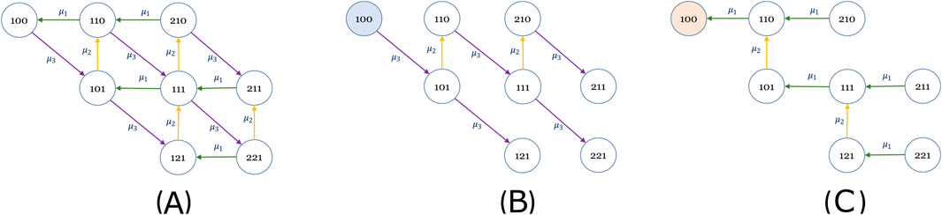
Figure 1. The graph (A) is based in Muth (1984) and it has the transition matrix Q, Equation 11. An arborescence rooted in state 100 (B) and an anti-arborescence ending in the same state 100 (C). The edges weights represent the mean service rates.

The type of graph represents Markov chains, namely directed graphs, where the edge (u,v) is also called an arc and is orientated (directed), where the vertex u is the origin and the vertex v is the target. The flow in orientated graphs can, therefore, only follow the specified direction, and in production systems, the flow leads the system to the next state immediately after a process that causes changes in the system. If G = (V, E) is a directed graph, then we define the inverse (inverted or transposed) graph G^-1= {V, E^-1} of G, for which E^-1= {(v,u)|(u,v)∈E} and v,u∈V. The weight w of each edge in the directed graphs distinguishes one edge from another. In Markov chains, it models the rate of transition from one state of the system to another. A path P= (v₀, v₁, …, v_n) of length n is denoted as the sequence of arcs from a vertex v₀ to a vertex v_n following the directions of the arcs, where the total number of vertices of the graph on the path is n + 1, starting at vertex v₀ and ending at vertex v_n. The arcs of the graph on the path are unique.

A tree is called a connected graph without cycles, i.e., acyclic. An origin tree is a tree whose vertex r is called the origin or root of the tree, see Figure 1B. Alternatively, the tree can be rooted at vertex r. A graph G’s spanning tree (arborescence) is called a subgraph T if it is a tree and contains all vertices of G. A graph G can only have a spanning tree if it is connected. In particular, for a directed graph G, a spanning tree rooted at vertex r is a subgraph that has a unique directed path from r to each vertex of G. By reversing the direction of all the edges of a spanning tree rooted at a vertex r so that they all point towards the root and not away from it, we get a different spanning tree, called an anti-arborescence.

Suppose the system modeled by a Markov Chain is represented by a directed graph G (V, E), where V is the set of vertices (the cardinal number of V is Ν) and E is the set of edges of the graph. In this case, one can construct the anti-arborescence of the system leading to node j (v nodes of the graph G), see Figure 1C. The anti-arborescence is the reverse spanning tree rooted at node v (Korte and Vygen, 2018), and it is defined in a directed graph G as the in-tree that ends in a single node (here, node v) of the graph. An in-tree is the subgraph C_v that represents a single tree that ends at node v and follows some edges of graph G but includes all nodes of graph G only once.

The anti-arborescence tree structure describes the successive transitions from an arbitrary initial state of the graph, k, to a final state, j. Furthermore, anti-arborescence can represent and enumerate all combinations of all possible transitions from any initial or transition node of graph G to the final state j.

The anti-arborescence contains all nodes of the graph, i.e., all Ν-states of the system corresponding to the states of the Markov chain, and it always has Ν-1 edges connecting the nodes of the graph. Each edge connecting two states (let us assume it starts in state i and ends in state k) is labeled e_ik and has a weight corresponding to the probability of transition from state i to state k, p_ik, and is labeled w(e_ik). Thus, each anti-arborescence forms a set with Ν -1 unique transition edges that connect each system state to the final state j and make it accessible from any other state within at most Ν -1 transitions.

Consider a graph G that represents the Markov chain that models a system in a stable state like, a model of a serial production line (Papadopoulos et al., 2009). The transition from one state to another is time-independent and corresponds to the transition rate from one state of the Markov chain to the next. Thus, if the system is in state i and transitions to state j and then to state k, the transition probabilities are determined by Equation 1 (Kolmogorov, 1956). The latter is expressed using the transition probabilities from one state to another from the transition probability matrix P and can be generalized for system transitions to several successive states of the Markov chain. From now on, these transition probabilities, i.e., the transition rates from one state to another, are assigned to the weights of the arcs of graph G to express the steady-state probabilities symbolically using the graph structure, starting from outer vertices and moving towards the end of the graph’s anti-arborescences, exploiting Equation 1.

$p_{ik}=p_{ij}·p_{jk},i<j<k(1)$

An anti-arborescence C in the direction of one of the N states of graph G occurs according to the probability with which the Markov chain moves from any state k of graph G to the final state. The transitions are independent events along the edges that form the anti-arborescence C. Due to independence, the probability of anti-arborescence C is given by the product of the probabilities of each edge of C, see Equation 2, which has N-1 terms, where w (e) expresses the probabilities of transition from one state to another. According to the Markov Chain Tree Theorem, these probabilities are the edge weights of the graph G (Evans, 2008).

$P^{Markov}\left(C\right)=\prod _{e\in C}w\left(e\right)(2)$

The P^Markov(C) probability should be normalized to express the probability of anti-arborescence C, P(C). The sum of all probabilities of the anti-arborescences of graph G, denoted C_G, must equal one, i.e., P(C_G) = 1. The ratio of the probability of the anti-arborescences for the state v divided by the probability of all anti-arborescences of the graph is the probability that the system is in the state v.

Any two anti-arborescences Α, Β, represent two different events C^A, C^B of the space Ω, and it holds P(C^A∪C^B) = P(C^A) + P(C^B), generalized in Equation 3. The union of all anti-arborescences of graph G is the complete set of all anti-arborescences of graph G, i.e., $\mathrm{\Omega }=C_G=\bigcup _{C\in C_G}C$. The probability of set Ω in combination with Equations 2, 3, therefore results from Equation 4.

$P\left(\bigcup _{i=1}^n{C}^i\right)={\displaystyle \sum _{i=1}^n}P\left(C^i\right)(3)$

$P\left(\mathrm{\Omega }\right)=P\left(C_G\right)=P\left(\bigcup _{C\in C_G}C\right)={\displaystyle \sum _{C\in C_G}}P\left(C\right)={\displaystyle \sum _{C\in C_G}}\prod _{e\in C}w\left(e\right)=1(4)$

Thus, the probability of any anti-arborescence C_i is equal to the probability of the transition of the Markov chain following the edges of C_i divided by the sum of the corresponding probabilities for each of the anti-arborescences in the graph G, given by Equation 5.

$P\left(C^i\right)=\frac{P^{Markov}\left(C^i\right)}{P\left(C_G\right)}=\frac{{\prod }_{e\in C^i}w\left(e\right)}{{\displaystyle {\sum }_{C\in C_G}}{\prod }_{e\in C}w\left(e\right)}(5)$

The three elements (Ω, A, P) form a probability space defined by the set of anti-arborescences of the graph G, a finite Markov chain, with a σ-field of subsets of Ω and a probability measure P defined in A.

Equation 6 gives the set Cj of all anti-arborescences that lead the system to state j, with a probability equal to the stationary probability ${\pi }_j$ of the underlying Markov chain modeling the system. All that remains is to find a way to identify all the anti-arborescences of graph G.

${\pi }_j=P\left(C_j\right)=\frac{{\displaystyle {\sum }_{C^i\in C_j}}P\left(C^i\right)}{P\left(C_G\right)}=\frac{{\displaystyle {\sum }_{C^i\in C_j}}{\prod }_{e\in C^i}w\left(e\right)}{{\displaystyle {\sum }_{C\in C_G}}{\prod }_{e\in C}w\left(e\right)}=\frac{{\displaystyle {\sum }_{C^i\in C_j}}{\prod }_{e\in C^i}w\left(e\right)}{{\displaystyle {\sum }_{k=1}^N}{\displaystyle {\sum }_{C\in C_k}}{\prod }_{e\in C}w\left(e\right)}(6)$

The product $\prod _{e\in C}w\left(e\right)$ forms the main terms of a monomial and is referred to below as the spanning monomial. Accordingly, the stationary probability π_j is a ratio of two polynomials. The numerator is called the spanning polynomial of state j, denoted as sp_j, and consists of the sum of the spanning monomials. If the transitions between the states have identical weights, i.e., transition rates, the monomials sum up and give a monomial coefficient in the spanning polynomial. All stationary probabilities have a common denominator called the spanning polynomial of the graph, denoted as sp_G. This denominator can be expressed as Equation 7, and following this symbolism, any stationary probability of the state j, π_j can be obtained in analytic or numerical form, as Equation 8 describes by the ratio of two polynomials.

${sp}_G={\displaystyle \sum _{j\in G}}s{p}_j(7)$

${\pi }_j=\frac{s{p}_j}{s{p}_G},j\in G(8)$

Computing the steady-state probability of Equation 8 requires extracting all spanning polynomials using any appropriate method for each graph state to form the sp_G polynomial, the denominator of each steady-state probability of the system state. Thus, the Algorithm can automatically provide the stationary probabilities of a Markov chain from its transition matrix in analytic form. The only requirement is that all anti-arborescences of the state transition graph be enumerated, and no further processing is required, such as solving systems of linear algebraic equations or solving differential equations. The solutions provided by the Algorithm are the exact closed-form solutions since all transition probabilities are included in the final solution, which is ultimately a ratio of two polynomials. Depending on the form of the weights on the edges of the graph G or the matrix P, i.e., whether they are in symbolic or numerical form, the stationary probability π_j that the system remains in the given state j is given symbolically as a mathematical formula or as a number respectively.

2.2 Description of the proposed algorithm

Given the transition matrix P for a system with Ν states modeled as a Markov process, the goal is to express stationary probabilities as mathematical relations in analytic form with closed-form equations. The sum of its elements equals one in each row of the matrix P. The matrix P can be rewritten into the corresponding graph G (V, E), which forms the background for searching all anti-arborescences at each vertex v∈V of the graph.

All transitions are written in the form of a list, and the arc, i.e., weighted edge, of each transition from state i to state j is supplemented by the weight w(e_ij), which corresponds to the probability p_ij from the matrix P. The graph, therefore, shows as many transitions as non-zero elements of the matrix P.

2.2.1 The Gabow and Myers’ algorithm

The first purpose of the Algorithm is to enumerate all anti-arborescences ending at each vertex of the graph. For this enumeration, is used any suitable algorithm, but in the present work for systems with many spanning trees, the algorithm of Gabow and Myers (1978) is adopted, which lists rooted trees at each vertex of the graph. The algorithm finds all the spanning trees of a directed graph rooted at a specific vertex, r, i.e., the state of the underlying Markov chain. The algorithm finds all the spanning trees containing a subtree T rooted at r. The process begins by selecting an edge e₁ that is directed from T to a vertex, not in T. Next, the algorithm finds all of the spanning trees containing $\mathrm{T}\cup$ e₁ and then deletes e₁ from the graph. This process is repeated for all edges e₂ to e_i that are directed from T to a vertex, not in T. Finally, the algorithm stops when the edge e_k that has just been processed is a bridge of the modified graph. This approach helps find a directed graph’s spanning tree. All the spanning trees containing T appear to have been found precisely once. If a spanning tree does not contain any e_j, j < k, then it must include the bridge Q, and the work of Gabow and Myers uses a method based on the depth-first search (see Sedgewick, 2001) to locate the bridge Q, i.e., the edge that if it is removed splits the graph into two separate graphs.

The algorithm selects edges e such that the tree T grows depth-first, aiming to add the edge e to T, which originates at the most incredible depth possible. The algorithm uses F, a list of all edges directed from vertices in T to vertices not in T, for growing T depth-first. Enlarging T is about invoking a procedure called GROW, which involves popping an edge e from the front of F and adding it to T. Procedure GROW also pushes a new edge, for $T\cup e$, onto the front of F. Additionally, when e is added to T, some edges are removed from F, and when e is removed from T, these edges are restored in F. The removal and restoration operations must leave the order of edges unchanged in F, or T will not grow depth-first. In addition to F, the algorithm uses lists FF. Every recursive invocation of GROW has a local FF list, which is used to reconstruct the original F list and managed as a stack. The algorithm also employs data structures for T, the current tree growing, adding new edges and vertices, and the spanning tree L, the output spanning tree containing all the graph’s vertices.

2.2.2 The algorithm’s basic steps

The Gabow and Myers’ algorithm is executed Ν times, the number of system states. However, Gabow and Myers’ algorithm is not designed to detect anti-arborescences. The latter requires the reversal of the direction of the graph edges, i.e., the edge e_ij and the weight w(e_ij) become e_ji, while the same weight w(e_ij) is kept. After this change, Gabow and Myers’ algorithm exhaustively finds all anti-arborescences starting from a vertex v and locates all arborescences rooted in this node of the reversed graph G. It also requires a record of the weights (transition rates) of each rooted spanning tree (arborescence) that match the original direction. In this way, the process finally generates the products of Equation 2. If these products have standard terms, algebraic operations can be performed to convert the products into monomials, i.e., spanning monomials, or polynomials, i.e., spanning polynomials.

The sum of all spanning monomials generated by the anti-arborescences forms a polynomial at each vertex. This spanning polynomial is the numerator of the stationary probability of the state. The sum of the spanning polynomials in each final state of the graph forms the spanning polynomial of the sp_G graph, which is the denominator of each stationary probability.

Using the spanning polynomial in each state and the spanning polynomial of the graph, the steady-state probabilities of each state j, π_j can be extracted as the ratio of these two polynomials according to Equation 8.

To summarize, the five basic steps of the algorithm are as follows, see Figure 2 for an overview of the Algorithm:

1. Using a suitable method, form the system transition matrix P and invert it, P^T, see Figure 2A.

2. Enumerate all N states of the table P^T and construct the original graph with N vertices and all information in a suitable data structure, see Figure 2A.

3. For each vertex of the graph j, perform the following, see Figure 2B:

a. Reorder the remaining vertices by first searching in depth starting from vertex j.

b. Find all spanning trees that end at vertex j using the Gabow and Myers algorithm.

c. For each spanning tree, form the corresponding monomial by multiplying the weights of the edges of the spanning tree and add all monomials that form the spanning polynomial of vertex j.

4. Add the spanning polynomial of all vertices that form the spanning polynomial of the graph, see Figure 2C.

5. Calculate the stationary probability for each state by dividing the spanning polynomial of state j, j∈{1, … , N}, by the spanning polynomial of the graph, see Figure 2C.

Figure 2

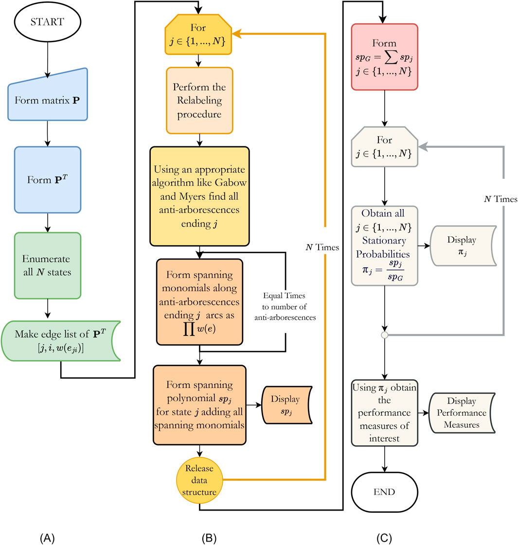
Figure 2. The flowchart of the proposed Algorithm. Basic steps 1 and 2 are depicted in (A). Basic steps 3a, 3b, and 3c are depicted in (B). Basic steps 4 and 5 are depicted in (C). The sequence of steps follows the chart flow, and the different colors distinguish them.

2.3 The detailed steps of the algorithm

The Algorithm, see Table 1 presents the automatic extraction of the symbolic stationary probabilities from a Markov chain in 27 algorithmic lines, see Algorithm. The Algorithm takes the transition matrix P of the system with N states as input with numerical or symbolic elements. The Algorithm’s output is the system’s stationary probabilities in numerical or symbolic form for each of the N states.

Table 1

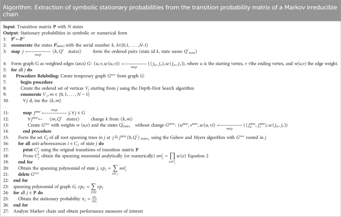
Table 1. The Algorithm for calculating the symbolic stationary probabilities.

As summarized above, the Algorithm’s steps are explained in detail and grouped into five basic ones.

2.3.1 Basic step 1

The Algorithm reverses the direction of the edges in Step 1 by transposing the matrix P, which has N states, so that Gabow and Myers’ algorithm can enumerate all the graph’s anti-arborescences. This change of direction preserves the weights of the edges so that the transition matrix and its transpose matrix have the same states and weights but alternate between the start and end transition states. For Gabow and Myers’ algorithm to work, each state must be assigned a consecutive integer number, starting with zero for the final state under consideration.

2.3.2 Basic step 2

Each state, therefore, has two attributes: a serial number, which was specified in line 2, and the pair (state identifier from the matrix P, expression of the state, e.g., state “s1”). Line 3 creates a list with integer numbers of states from 1 to N-1 and their names with character strings. These elements must remain unchanged to extract the stationary probabilities at the end. The transition matrix graph is constructed with these features, where each vertex is represented by the pair (state id, state expression string), and each edge is represented by the two nodes at the beginning and end of the transition and the transition weight. This graph is created in line 4 and remains unchanged throughout the Algorithm as the reference graph.

2.3.3 Basic step 3

That is followed by a loop executed N times, lines 5–22, in which each state of the transition matrix P, i.e., a vertex of the graph G, is considered the final state j and the spanning polynomial for this state is extracted. At the end of the loop, all spanning polynomials for each state have been extracted so that the spanning polynomial of the graph, sp_G, can be determined as the sum of the spanning polynomials of the individual states.

2.3.3.1 Basic step 3.a

The processing of each state begins with a procedure called Relabeling (lines 6–14). During the Relabeling procedure, starting from vertex j of the graph representing the considered state j∊{0,1, … , N-1} in which the spanning polynomial is extracted, the vertices of the graph are ordered based on the Depth-First Search (line 8). The Algorithm temporarily renames vertices with this layout list (lines 9 and 10). However, it retains the strings naming the states and the transition weights regarding graph G, which acts as a reference graph containing all the information about the structure of the underlying Markov chain (lines 11 and 12). The new vertices create a new temporary graph G^new from which rooted spanning trees are extracted whose root has a temporary ID from the Relabeling process equal to zero (line 13). All other elements of the graph G^new, i.e., the edge weights and the names of the vertices, remain unchanged. The procedure ends at line 14 when all N vertices have been renamed.

It is crucial to leave the original graph unchanged to obtain a consistent rendering of the spanning trees and extract the correct formulas expressing the stationary probabilities, i.e., the solutions of the equilibrium equations derived from the transition matrix P. That is because, although the Gabow and Myers’ algorithm treats the graph’s vertices as a label with an ascending number, this does not work in the same way if the vertices and edges carry information, i.e., states and transition rates between states. It is vital to obtain this information to solve the equilibrium equations. Thus, if the Relabeling procedure is used, the original graph is transformed temporarily N times, as many times as the number of states in the transition matrix P. So, preserving the original graph leads to the correct monomials corresponding to the transition matrix P. Otherwise, the Gabow and Myers algorithm provides all spanning trees of the graph. However, these do not correspond to the correct monomials that solve the equilibrium equations of the matrix P.

2.3.3.2 Basic step 3.b

In line 15, the Algorithm forms all spanning trees rooted in state j of the graph G^new. For this purpose, the algorithm of Gabow and Myers is executed on the graph G^new, where vertex j is the root. That means that all spanning trees that start from vertex j and include all other vertices of the graph Gnew are recorded. These trees are the arborescences of the graph G^new, but with the direction reversed due to line 1 of the Algorithm.

2.3.3.3 Basic step 3.c

That is followed by a loop executed as often as the number of spanning trees identified for state j in line 15 of the Algorithm (lines 16–19). The purpose of the loop is to convert each spanning tree into a spanning monomial by taking the product of the weight, i.e., the transition rate, of each edge of the spanning tree times the weights of all other edges that form the spanning tree. If the weights are symbols, the product is a string, and the spanning monomial is treated as a symbolic mathematical term. If the weights are numbers, the monomial is a number and is treated as such. All resulting spanning trees are printed in line 17 in the correct order (anti-arborescences) of the initial transition matrix P. In line 18, the spanning monomials for each tree are extracted. The loop ends at line 19 when all the temporary graph G^new spanning trees have been elaborated.

In line 20, the spanning polynomial of state j is extracted. The loop that started in line 5 is completed for state j with the destruction of the temporary graph G^new in line 21. The same procedure is applied for state j+1 until the states of the Markov chain are exhausted (line 22).

2.3.4 Basic step 4

Then, by summing all spanning polynomials for each vertex j, the Algorithm proceeds to form the spanning polynomial sp_G of the entire graph G (line 23). The sp_G is the denominator of every stationary probability of the matrix P.

2.3.5 Basic step 5

There follows a loop that is executed N times (lines 24–26), in which for each state j of the transition matrix P, i.e., a vertex of the graph G, its stationary probability is extracted as the ratio of the spanning polynomial of state j divided by the spanning polynomial sp_G of the graph G. After the extraction of the stationary probabilities in symbolic or numerical form, they can be used to analyze the Markov chain to obtain performance measures of interest (line 27).

2.4 The complexity of the algorithm and the number of spanning trees

The Algorithm’s complexity is equal to the complexity of the Gabow and Myers’ algorithm. That is because the Relabeling process (a Depth-First Search) occurs only once for each state. At the same time, the “bridge search” (the stopping criterion for the Gabow and Myers algorithm) is performed millions of times as the graph is enlarged. Therefore, the Gabow and Myers’ algorithm dominates the extraction of anti-arborescences.

The algorithm of Gabow and Myers was presented in the work of Gabow and Myers (1978). Its complexity is given as O(V + E + EN’), where V is the number of vertices, E is the number of edges, and N’ is the number of all spanning trees in a graph. Thus, the Algorithm’s time complexity is O(V + E + EN’) and space complexity is O(V + E). For the worst case of a fully connected directed graph, let n be the number of vertices. In this case, $E=n\left(n-1\right)$ and $N’=n{n}^{n-2}$. Then the time complexity of the method is $O\left(n+n\left(n+1\right)+n^2\left(n-1\right)n^{n-2}\right)$ or $O\left(n^n\right)$. Working the same way the memory complexity is $O\left(n^2\right)$. In the case of serial production lines without intermediate buffers, it is asymptotically true that the number of states is a function of the number of stages K and $n={2.618}^K/2.236$ (Muth, 1984). Therefore, the time complexity for such systems is $O\left({2.618}^{K{2.618}^K}\right)$ and memory complexity is $O\left({6.854}^K\right)$. However, due to the assumptions of Markovian models, the real values of transitions are smaller than the theoretical ones. For example, in the case of K = 10 stages, our team analyzed the underlying graph and found 6,765 states and 32,960 transitions between states, a number significantly smaller than the theoretical 45,758,460 that applies to the fully connected graph. However, the hyper-exponential increase in complexity limits the method to small graphs and thus to production systems with few stages, which are used as structural elements for other numerical methods.

That means that the complexity of the analytical solution of stationary probabilities is significantly higher than that of the numerical solution of stationary probabilities, where the complexity measure is the number of states of the Markov chain. In the numerical solution, the probability constantly shrinks to a number in the calculations; in contrast to the analytical solution, the probability is expressed as the ratio of two ever-increasing polynomials. However, once the stationary probabilities are available in symbolic form, the output results are significantly faster than numerical methods without special software requirements.

Another parameter related to the nature of the problem and the size of the exact mathematical relations in systems modeled with Markov chains is the total number of spanning trees present in a graph. That affects the polynomials’ and the formulas’ final sizes. There is an upper bound on the number of spanning trees that results from the case of a complete graph where all vertices are connected. Cayley’s formula gives this (Takács, 1990), which states that the number of anti-arborescences N_sp for each vertex equals N_sp = nⁿ⁻² where n is the vertices number.

Generally, the number of spanning trees in a directed graph for the frequent case in some transitions between states or exchangeable edges that do not exist is estimated by a variation of the matrix-tree theorem, see the book Van Lint and Wilson (2001). The number of spanning trees κ(G) in a directed graph G= (V, E) is equal to the determinant of a suitable matrix, the Laplacian matrix L of the graph G. L is defined by L = D-A, where D is the following matrix given by Equation 9:

$D=\left(\begin{array}{ccc}{d}_1& \dots & 0\\ ⫶& \ddots & ⫶\\ 0& \dots & d_n\end{array}\right)(9)$

Where, d_i = d+(v_i)= #{j∈V|(i, j) ∈ E}, the outer degree of vertex v_i and n is the number of system states, and the symbol # denotes the number of output edges from vertex i. The matrix A is the adjacency matrix of G without weights, defined as A=(α_ij) where, $a_{ij}$ is given in Equation 10.

$a_{ij}=\left\{\begin{array}{c}0\text{\hspace{0.5em}if\hspace{0.17em}}\left(v_i,v_j\right)\notin E\\ 1\text{\hspace{1em}if\hspace{0.17em}}\left(v_i,v_j\right)\in E\end{array}\right.(10)$

The number of directed spanning trees rooted in the node r of the graph G, κ(G, r) is: κ(G, r) = det-L_r where L_r is the Laplacian matrix L from which the row r and column r have been removed. The sum of the spanning trees for all vertices of the graph is the number of all spanning trees equal to the number of anti-arborescences of the graph. Even if the transition matrix of the Markov chain is sparse, applying the method based on the matrix-tree theorem to calculate the number of spanning trees yields a colossal number of spanning trees.

2.5 The Relabeling procedure

In Figure 3A, we see graph G, formed in line 4 of the Algorithm. Each vertex is the corresponding number of the state from the matrix P, and the string refers to the specific problem (it is useful when considering a system with many states). Above each vertex is the serial number of the vertex from line 2 of the Algorithm, see Table 1.

Figure 3

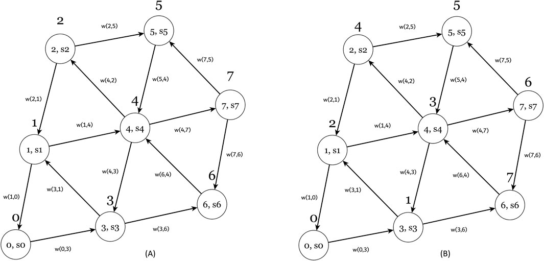
Figure 3. Relabeling a graph G (A) on the left to form the graph G_new (B) on the right, where the state 0 is considered final. The graph is based on the one in Muth (1984).

Figure 3 shows the graph presented in Muth (1984) with the direction of the edges reversed and the information that is stored in data structure of the Algorithm. It is noted that the graph is the same as the graph in Figure 1A which preserves the original edge direction. The purpose of the figure is to show the change that the Relabeling procedure has on the structure of the graph, as well as the amount of information that should be stored for the Algorithm’s execution. The Relabeling procedure is applied to Figure 3B, where the vertices are given an ascending numbering based on the Depth-First Search, forming the graph G^new, of the Algorithm. The other graph elements, such as states, strings, edges, and edge weights, remain unchanged.

The difference between the two diagrams is in the numbering above the vertices, represented by circles. This numbering is done using the Depth-First Search algorithm, while all other information remains the same. Each circle contains the original numbering of the graph, i.e., the string describing the state of the Markov chain. The edges are labeled with weights of the form w (start, end), where the start is the start vertex of the arrow, and the end is the end vertex, i.e., the initial state of the Markov chain and the final state, respectively, where the arrow represents the transition. The value of the weight w of the arrow indicates the transition rate from the initial state to the final state. If w is a character string, the Algorithm results in a symbolic formula. If w is a numeric value, the operations can be performed with a numeric result. All values of the graph, i.e., vertex contents and edge weights, are derived from the initialization of the original graph, and the use of a suitable data structure to store these values along with the numbering from the Depth-First Search algorithm should be considered when implementing the Algorithm with the desired programming language.

The Relabeling procedure does not affect the Algorithm’s output (the result), but the time it takes to execute it. This practical observation emerged from experiments with transition matrices corresponding to relatively large graphs. The algorithm of Gabow and Myers enumerates all spanning trees that have their root in a state, i.e., in a vertex, and relies on a Depth-First Search procedure, a well-known algorithm (see Sedgewick, 2001), to find a bridge in the graph (Gabow and Myers, 1978). In the experiments conducted, each time when the root of the graph changes, there is a possibility that the number of iterations of the Depth-First Search increases or decreases. Since the graph’s vertices are examined according to their ascending number, Relabeling reduces the number of manipulations required by the Algorithm to identify the edge that forms the bridge. This reduction in manipulations reduces the execution time of the Algorithm when enumerating the spanning trees in the graph set. The Relabeling procedure does not significantly affect small graphs but should be used when considering large graphs in more complex systems.

3 Examples of the proposed algorithm

In this section, two examples are given to help understand the functionality of the proposed Algorithm for deriving stationary probabilities in symbolic form. An example based on serial production lines, which generates a polynomial part of the throughput formula of Hunt (1956) iconic work, is given in Section 3.1. In Section 3.2, the proposed Algorithm is applied to a two-stage line with one slot buffer, which provides performance measures in symbolic form.

3.1 General example of short serial production lines

The example presented in this Section comes from Operations Research and was introduced by Hunt (1956), where the objective was, among other things, to find the throughput of a system with three machines without intermediate buffers. Hunt gave an exact solution of the system in symbolic form that satisfies the equilibrium equations of the underlying Markov chain. This example was chosen because Hunt provided the equations for maximum system utilization and throughput in a ratio of two polynomials with particular characteristics. After the publication of his work, a question that has occupied the research community for seven decades is whether other performance measures of serial production lines modeled with Markov chains can be expressed with closed-form equations. The proposed algorithm explains the structure of Hunt’s polynomials and provides an affirmative answer to whether there are closed-form equations that describe all performance metrics of systems computed using numerical methods, mainly from linear algebra. The example in the present work is given to present and explain some technicalities of the proposed algorithm and how to formulate Hunt’s polynomial through the analysis of transition rate diagrams.

The modeling of the system is presented in Papadopoulos et al. (2009). The workpieces are picked sequentially by the three machines. When the parts are finished processing on each machine, they move on to the next one until they become finished products. Each machine can be in three possible states: 0: idle, 1: working, and 2: blocked. The system’s state consists of three digits, i.e., the composition of the states of the individual machines following the above indicators. Here, the spanning monomial for system state 121 will be given, which state is interpreted as the first machine working, the second machine blocked, and the third machine working.

According to the model, the state space S contains eight states, $S=\left\{100,101,110,111,121,210,211,221\right\}$. The transition matrix of the system is the Q in Equation 11, where the states are in the same order as given in S. The elements are the mean service rates of the machines where their service time are exponentially distributed random variables, i.e., μ_i, i = 1,2,3. The elements of the prime diagonal indicate that the system remains in the same state. For instance, when the system is in state 101, transit to state 100 by a rate μ₃ or to state 111 by a rate μ₁ and remains in state 101 by a rate equal to the sum (μ₁+μ₃).

$\mathbf{Q}=\left(\begin{array}{cccccccc}-{\mu }_1& 0& {\mu }_1& 0& 0& 0& 0& 0\\ {\mu }_3& -\left({\mu }_1+{\mu }_3\right)& 0& {\mu }_1& 0& 0& 0& 0\\ 0& {\mu }_2& -\left({\mu }_1+{\mu }_2\right)& 0& 0& {\mu }_1& 0& 0\\ 0& 0& {\mu }_3& -\left({\mu }_1+{\mu }_2+{\mu }_3\right)& {\mu }_2& 0& {\mu }_1& 0\\ 0& {\mu }_3& 0& 0& -\left({\mu }_1+{\mu }_3\right)& 0& 0& {\mu }_1\\ 0& 0& 0& {\mu }_2& 0& -{\mu }_2& 0& 0\\ 0& 0& 0& 0& 0& {\mu }_3& -\left({\mu }_2+{\mu }_3\right)& {\mu }_2\\ 0& 0& 0& {\mu }_3& 0& 0& 0& -{\mu }_3\end{array}\right)(11)$

A graph is an abstract construct based on set theory and can be expressed in various forms. The shapes are not as important as the connections between vertices and the weights of those connections. Thus, Figure 4 shows the graph where all transitions are written in list form. Therefore, 14 transitions between two states are recorded, forming the edges or arcs of the graph of the Markov chain. The corresponding transition rate is recorded for each transition, which is the weight of the transition edge from one state to another. The list of the 14 edges is shown on the left in Figure 4A, with the direction of the graph’s edges shown in the center in Figure 4B. Finally, on the right if Figure 4C, the graph is displayed. Colors are used to remain unchanged to facilitate the reading of the shapes. It is noted that Figure 4C is the same with Figure 1A.

Figure 4

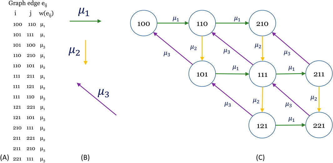
Figure 4. The state-to-state transition diagram for the Q matrix of Equation 11. (A) On the left is the matrix in edge-list form; (B) the original transition direction for each average service rate μ_i and (C) the graph of the system without the self-loops of occupation in the same state.

The Algorithm aims to list all the anti-arborescences at each vertex of the graph. For this purpose, the algorithm of Gabow and Myers will be used, which enumerates the rooted trees at a vertex of the graph. This algorithm is used as many times as the number of the system states. However, the Gabow and Myers algorithm is not designed to identify the spanning trees ending in a specific vertex. Therefore, the direction of the graph’s edges must be reversed, i.e., a transition’s initial and final states must be reversed, as shown in Figure 5A. The resulting graph Figure 5B is the graph of the inverse matrix of the Markov chain transitions. Then, the Gabow and Myers algorithm can be applied, and exhaustively, it will correctly identify all the anti-arborescences starting from each vertex of the graph individually.

Figure 5

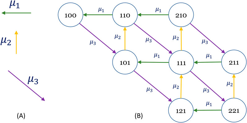
Figure 5. The graph of Figure 4 shows the edges in the reverse direction. (A) The reversed transition direction for each average service rate μ_i and (B) the graph of the system. It corresponds to the transpose matrix Q^T and is used to find all the anti-arborescences of the Q matrix using the Gabow and Myers’ algorithms.

Thus, the Gabow and Myers algorithm is executed as many times as the vertices of the graph, i.e., the states of the Markov chain. The resulting anti-arborescences should be inverted to form the spanning trees ending in a vertex, as shown in Figure 6, where all spanning trees ending in vertex 121 are shown i.e., ${sp}_{121}^1,{sp}_{121}^2,{sp}_{121}^3,{sp}_{121}^4,{sp}_{121}^5,{sp}_{121}^6$ in Figures 6A–F respectively. Note that for this graph, this vertex has six spanning trees, which is the least number of spanning trees compared to any other vertex in the graph. The product of the weights of the edges of a spanning tree in Figure 7A is the same as the product of the corresponding anti-arborescence that created it in Figure 7B and can be written as a monomial, as shown in Figure 7C which corresponds to sp4 121 depicted in Figure 6D. All the monomials obtained in this way are summed. In the presented case, i.e., all the monomials correspond to the six spanning trees of Figure 6, then the spanning polynomial of Equation 12 is formed. Note that this polynomial is included in the formula that Hunt published because the stationary probability of state 121 participates in the equilibrium equations. The 121-state stationary probability can be estimated when all the spanning polynomials of the graph are formed, i.e., for all states of the graph or Markov chain, so it is possible to create the stationary probabilities of Equation 6.

$s{p}_{121}={\mu }_1^2{\mu }_2^4{\mu }_3+{\mu }_1^3{\mu }_2^3{\mu }_3+2{\mu }_1^2{\mu }_2^3{\mu }_3^2+{\mu }_1^3{\mu }_2^2{\mu }_3^2+{\mu }_1^2{\mu }_2^2{\mu }_3^3(12)$

Figure 6

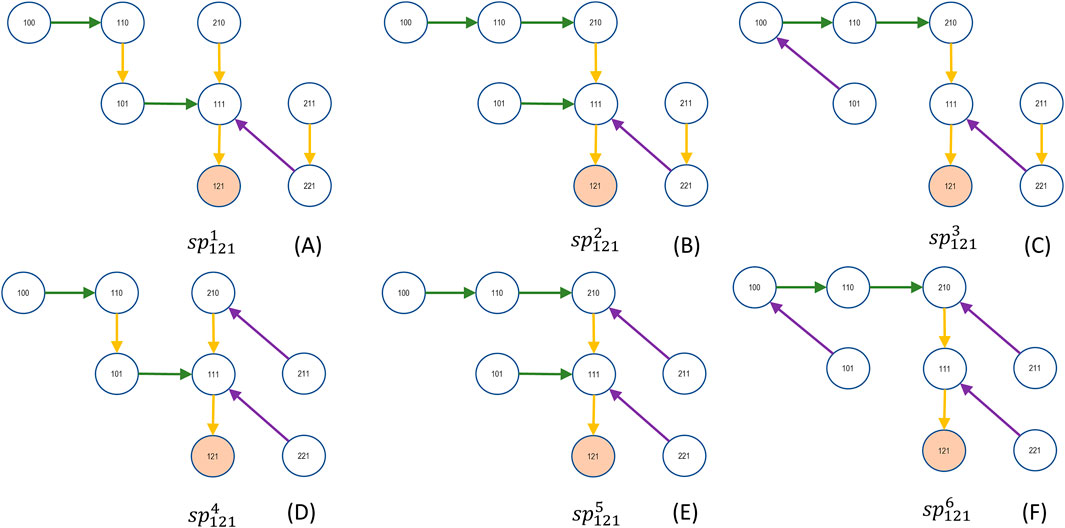
Figure 6. The six spanning trees (A–F) end in state 121. The exponents numbered one through six correspond to the paths of the computation tree in Figure 8.

Figure 7

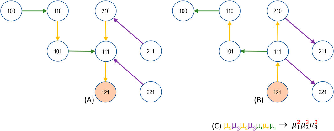
Figure 7. The spanning tree of state 121 (A) on the left and the corresponding anti-arborescence (B) on the right are accompanied by the product of the edges that form the spanning monomial. ${sp}_{121}^4$ (C).

The illustration of the computation tree (Gabow and Myers, 1978; Griffor, 1999) in Figure 8 is of great interest. There, the operation, the evolution, and the implementation of the Gabow and Myers algorithm are presented. The algorithm starts from the root, i.e., state 121, and systematically finds all the graph’s spanning trees (anti-arborescences due to edge reverse). The GROW function of the Gabow and Myers algorithm is triggered at each node of the computation tree, and a new vertex is inserted into the spanning tree. Each node has a branching list; the list that records the algorithm’s path creates a recursive call of the function GROW to record all spanning trees. The spanning tree formation starts from the T₁ path and ends at the T₆ path. Thus, the generated computational tree describes a non-deterministic Touring machine, for each graph vertex, corresponding to a computational tree. The computational trees form a forest containing every possible transition and state in the underlying Markov chain that models the system.

Figure 8

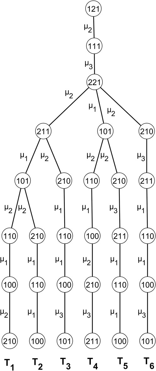
Figure 8. The computation tree of the anti-arborescences is rooted in state 121. Each path from root to leaf of the tree corresponds to the same numbered spanning tree in Figure 6.

3.2 Example of short serial production line

The example of this Section presents a serial production line of two stages with one slot intermediate buffer, i.e., intermediate storage spaces of a specific capacity located between machines. The production line layout is shown in Figure 9A. Buffers temporarily store semi-finished products when the next machine is working, thus preventing the previous machine from blocking. Blocking occurs when the semi-finished products in the buffer have reached their capacity limit, and there is no space to accept the last piece processed by the previous machine. The previous machine is blocked until space is freed up in the buffer by moving a piece to the next machine. The piece from the previous machine is then fed into the buffer, and the machine starts working again if a piece is available. In front of the first machine in the system, there is a continuous supply of raw materials, so the first machine is never starved. Similarly, after the second machine, there is ample space for storing the final products of the line, so the last machine in the system is never blocked.

Figure 9

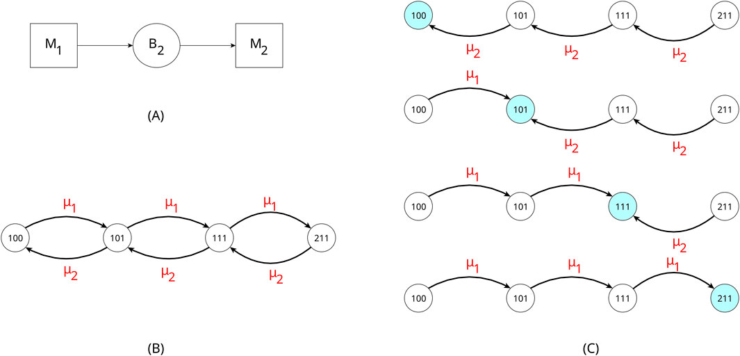
Figure 9. Serial production line (A). The state-to-state transition diagram of system (B), and the four anti-arborescences (C) each for each state of Q1 of Equation 13.

The states of the machines are S = {0: starved, 1: working, 2: blocked} and the buffers are B = {0: empty, 1: 1 position occupied, all positions occupied, equal to the buffer capacity}. The state of the system will be M₁B₂M₂, where M_i, i = 1,2 is the state of machine i and B_i, i = 2 is the state of buffer B of machine i. The machines work under an exponential distribution with mean service rates equal to μ₁ and μ₂, respectively. The system is modeled as a Markov chain with ${\mathbf{Q}}_{\mathbf{1}}$ transition rate matrix, Equation 13. The transition rate diagram is depicted in Figure 9B, and the four anti-arborescences are depicted in Figure 9C. It is noted that although the Algorithm solves the system, it is easy to obtain the spanning trees by hand due to the simplicity of the transition rate diagram. For every state, the spanning polynomial is equal to the spanning monomial ${sp}_j,j\in \left\{100,101,111,211\right\}$, i.e., the product of arcs weighs equals the mean service rates of the machines, see Equation 14, and the spanning polynomial $s{p}_G$ of the graph is the summation of the spanning monomials, see Equation 14.

${\mathbf{Q}}_{\mathbf{1}}=\left(\begin{array}{cccc}-{\mu }_1& {\mu }_1& & \\ {\mu }_2& -\left({\mu }_1+{\mu }_2\right)& {\mu }_1& \\ & {\mu }_2& -\left({\mu }_1+{\mu }_2\right)& {\mu }_1\\ & & {\mu }_2& -{\mu }_2\end{array}\right)(13)$

$\begin{array}{c}s{p}_{100}={\mu }_2^3\\ s{p}_{101}={\mu }_1{\mu }_2^2\\ s{p}_{111}={\mu }_1^2{\mu }_2\\ s{p}_{211}={\mu }_1^{3}s{p}_G=s{p}_{100}+s{p}_{101}+s{p}_{111}+s{p}_{211}={\mu }_2^3+{\mu }_1{\mu }_2^2+{\mu }_1^2{\mu }_2+{\mu }_1^3\end{array}(14)$

The maximum utilization of the system is the stationary probability of the system where the first machine is in work state, Equation 15.

${\rho }_{\mathit{max}}=\frac{{\displaystyle {\sum }_{\left.j\in G-\left\{s\right.p_{211}\right\}}}s{p}_j}{s{p}_G}=\frac{{\mu }_2^3+{\mu }_1{\mu }_2^2+{\mu }_1^2{\mu }_2}{{\mu }_2^3+{\mu }_1{\mu }_2^2+{\mu }_2+{\mu }_1^3}(15)$

Hunt provided a general formula for maximum utilization of a serial production line with intermediate buffers in (Hunt, 1956).

Hunt (1956) provided a general formula for maximizing the utilization, ${\rho }_{\mathit{max}}$ of a serial production line with intermediate buffers and expressed it as a function of the buffer capacity q, wherein the present example is q = 2. He distinguished two cases:

The first case is when μ₁ = μ₂ and the ${\rho }_{\mathit{max}}$ is given by Equation 16. It is easy to show that for μ₁ = μ₂, Equation 15 becomes 3/4, equal to the equation of Hunt for q = 2, i.e., buffer capacity equal to 1.

${\rho }_{\mathit{max}}=\frac{q+1}{q+2}(16)$

The second general case is when μ₁≠μ₂ where the maximum utilization is given by Equation 17, where in this example q = 2. Again, with some algebra, it can be shown that Equations 15, 17 are equivalent proving the correctness of Algorithm results.

${\rho }_{\mathit{max}}=\frac{{\mu }_2\left({\mu }_1^{q+1}-{\mu }_2^{q+1}\right)}{{\mu }_1^{q+2}-{\mu }_2^{q+2}}(17)$

Equation 18 gives the throughput of the system of two machines with one intermediate buffer of one slot, $X_2^1$, where it is noticeable the sum of the exponents of the numerator is equal to four. The sum of the exponents of the denominator is equal to three due to the state transition diagram structure and the throughput definition, which is produced by the product of the first machine’s mean service rate and the stationary probability of the first in-state work. i.e., non-blocked.

$X_2^1={\mu }_1{\rho }_{\mathit{max}}={\mu }_1\frac{{\displaystyle {\sum }_{j\in G-\left\{211\right\}}}s{p}_j}{s{p}_G}=\frac{{\mu }_1{\mu }_2^3+{\mu }_1^2{\mu }_2^2+{\mu }_1^3{\mu }_2}{{\mu }_2^3+{\mu }_1{\mu }_2^2+{\mu }_1^2{\mu }_2+{\mu }_1^3}(18)$

The results of Equation 18 were compared with the results of the MARKOV algorithm contained in the software Prodline (Papadopoulos et al., 2009) and for 196 cases of systems derived from the Cartesian product of the average service rates μ₁, μ₂ ∊ {0.2, 0.3, …, 1.5}. These configurations include balanced and unbalanced production lines. The results were run on the same computer, with Equation 15 results estimated in fractions of a second, while with Prodline, the same results took 6 min and 44 s for the estimation. This fact shows the usefulness of equations as building blocks in other methods for estimating the performance of larger production systems, regardless of the time required to find the equation since it can be used quickly and with low software requirements. The comparison of the results of the two methods gave a Mean Absolute Error of 2.82 10⁻⁷. That error is due to the rounding done by the exact MARKOV algorithm to six decimal places. At the same time, the equation reaches the limits of computational accuracy, with the results in the comparison given to 17 decimal places using Python programming language. The Mean Squared Error of the results is 2.73 10⁻¹³, the Mean Absolute Percentage Error is 5.86 10⁻⁷, and the Pearson Product-moment Correlation Coefficient is 0.999999, see Figure 10 where the plot of the results for the throughput $X_2^1$ of Equation 18, denoted as $X_2^1\text{Formula}$ versus the results of the MARKOV algorithm throughput $X_2^1$ estimation denoted as $X_2^1\text{MARKOV}$ is shown.

Figure 10

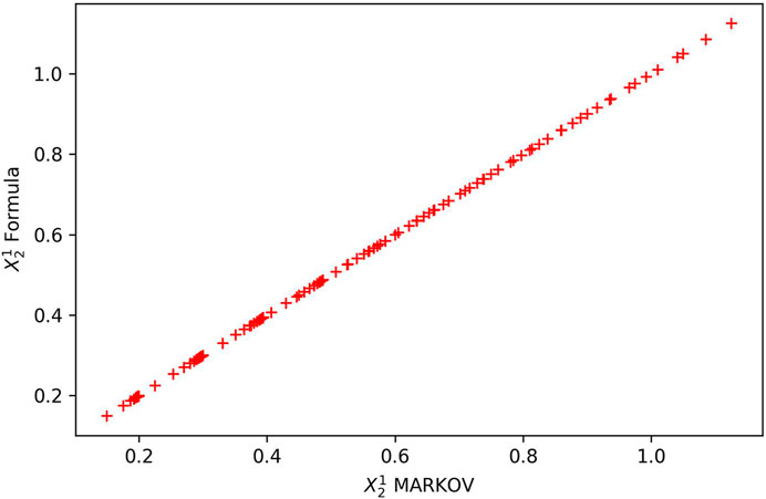
Figure 10. The plot of the196 cases results of Equation 18 formula against the MARKOV algorithm (Papadopoulos et al., 2009) for the throughput $X_2^1$ of a production line of two stages with one slot intermediate buffer. The results accumulate in 45° diagonal, showing equivalence.

Extending Hunt’s work, some equations of interest and metrics can potentially be used for system design, simulation, or development of decomposition methods and can easily be obtained since the spanning polynomials are available. For example, the probability that the first machine is blocked ${Bl}_1$ is given by Equation 19, the probability that the buffer of the second machine is full ${B_1}^f$ is given by Equation 20, and the work in the process of the system, $\overline{WIP}$ is given by Equation 21. The more complex the system under consideration, i.e., the transition matrix P has more N states, the more equations can be used depending on the desired result.

${Bl}_1=\frac{{sp}_{211}}{s{p}_G}=\frac{{\mu }_1^3}{{\mu }_2^3+{\mu }_1{\mu }_2^2+{\mu }_1^2{\mu }_2+{\mu }_1^3}(19)$

${B_1}^f=\frac{{sp}_{111}}{s{p}_G}=\frac{{\mu }_1^2{\mu }_2}{{\mu }_2^3+{\mu }_1{\mu }_2^2+{\mu }_1^2{\mu }_2+{\mu }_1^3}(20)$

$\overline{WIP}=\frac{s{p}_{100}+2s{p}_{101}+3s{p}_{111}+3s{p}_{211}}{s{p}_G}=\frac{{\mu }_2^3+{2\mu }_1{\mu }_2^2+{3\mu }_1^2{\mu }_2+{3\mu }_1^3}{{\mu }_2^3+{\mu }_1{\mu }_2^2+{\mu }_1^2{\mu }_2+{\mu }_1^3}(21)$

4 Discussion

Markov processes have long been used to model systems. The proposed method uses graphs representing these processes to extract mathematical models based on the Markov property. That is done by transforming the graphs from an illustration tool into a powerful computing tool. A spanning tree can represent the stationary probability of a state in the form of anti-arborescence ending in a graph vertex. The spanning tree holds information in weights that encode transition probabilities or rates at its edges.

The methodology uses anti-arborescences to extract symbolic formulas for systems. Previous works have achieved this using linear algebra or methods of symbolic regression, like genetic programming, which uses spanning trees in another context, or genetic algorithms (Boulas et al., 2021). The resulting formulas are ratios of two sets - the anti-arborescences ending in a graph vertex and all anti-arborescences in the graph explaining the terms in Hunt (1956). If simple variables are used, polynomial ratios are formed with the sum of exponents equal to the number of states minus one. Similar graphs for different systems with simple variables result in similar formulas.

Many papers in the past have addressed the problem of finding suitable closed-form mathematical formulas that can express the performance metrics of systems trying to address key points for the efficient operation of production lines. It is especially crucial to do so during the design or reprogramming phase of a production line. Researchers have devoted significant effort to producing simple functions expressing the production line’s throughput. Simple equations empower the designer or directors of the production line. There have been parallel efforts to find exact mathematical relationships that address the same problem. The present method for complex systems derives mathematical relationships that require a lot of computing time. However, once a mathematical relation is found, its use is superior in execution speed to numerical methods, which also is helpful when training data are produced for use in AI methods. The proposed method solves the system and expresses all stationary probabilities in symbolic form and all performance metrics. These can be used in the design and testing of simulations or the development of decomposition methods. This paper shows that closed-form functions can express all performance metrics of systems modeled by Markov chains. Future research efforts through graph theory will undoubtedly result in more straightforward relations in terms of accuracy and size. Numerical methods are not so appropriate for developing empathy in production line operations or for handling difficult, unbalanced production lines.

The method can be used in small systems to discover symbolic formulas in various problems like production lines, supply chains, or inventory problems. These formulas can contribute to decision-making, and recursive use can help solve larger systems. Graph theory results can be added to the arsenal of researchers working on such issues. As the number of states of the Markov processes increases, the number of graph-spanning trees increases tremendously, making the method intractable for practitioners, leaving this task to other approaches, such as intelligent methods. However, the method brings new possibilities for understanding various stochastic processes in a way that ultimately reduces to an enumerative process within the widely studied field of graphs. That creates great potential for further research and statistical investigation of phenomena to obtain approximate but highly accurate relationships that provide adequate intuition and understanding of phenomena. For example, the fact that the actual transitions between states are significantly smaller than those of a fully connected directed graph suggests a topology and internal structure in the graph that should be analyzed to explain better production problems, such as the bowl phenomenon, which significantly affects production lines and has a significant economic impact.

This method could create future benchmarking tests for robust computing systems, including quantum computers. Combining exact numerical answers about stationary probabilities of production lines using algorithms such as MARKOV (Papadopoulos et al., 2009) and the analytic solution could be attractive for creating benchmarking problems or algorithms that can test computational systems such as quantum computers (Steane, 1998). It compares the time it takes to find the anti-arborescences and the accuracy of the results. The present work’s examples show that the size of the exact closed formulas increases rapidly, making it a computational challenge for computers that may not have been invented yet.

Thanks to Gabow and Myers’ algorithm, the proposed algorithmic approach is based on automata theory, which combines Markov chains and data structures such as trees and graphs. This aspect is worth exploring. The computation tree in Figure 6 refers to a non-deterministic Turing machine; see, for instance Griffor (1999). From this point of view, the proposed algorithm’s results, i.e., the spanning polynomials, are detailed operating instructions for a production line describing the transitions along the anti-arborescences.

The size of the exact closed-form formulas expressing the stationary probabilities and performance measures is enormous, making AI-oriented methods attractive for forming approximate solutions for performance measurement in problems of interest. Better sampling into a graph’s enormous population of spanning trees is also interesting for artificial intelligence techniques, as it is relevant for building training sets and extracting better results, i.e., formulas or other predictive models.

5 Conclusion and further research

An Algorithm has been developed to express the stationary probabilities of a Markov process in either analytical or numerical form. The Algorithm is based on recording all the anti-arborescences present in the graph, representing the Markov process’s transition matrix. To do this, the edges whose weights represent the transition probabilities from one state to another are inverted. Then, all the spanning trees rooted in the considered state are identified using the Gabow and Myers’ algorithm. The weights of each spanning tree or anti-arborescence in the original graph form a product that gives the probability of transition from any vertex to the considered state, i.e., the last vertex of the anti-arborescence. The sum of the probabilities in a final state gives the corresponding stationary probability. Finally, all probabilities are normalized based on the sum of all anti-arborescences of the graph. When each weight is specified as a variable, the stationary probabilities are obtained in symbolic form.

Some well-known examples from the operations research literature have shown that the Algorithm provides the exact solutions for the systems of equations that solve the Markov process. The exact solutions are closed-form formulas, usually polynomial ratios (depending on the form of the variables), which increase in size at an exponential rate as the number of states of the Markov process increases. For this reason, a series of small examples have been used to demonstrate the application of the method. The Algorithm generates the analytic formulas that express the probabilities in a graph, including the stationary probabilities of the states of the underlying Markov process. This formation of the probabilities is done by enumerating anti-arborescences without using other mathematical tools such as differential or integral calculus.

The paper Boulas et al. (2024), corresponds to Part II of this work and demonstrates the efficacy of the proposed method in finding the formulas partially introduced in Hunt (1956). The present method treats these formulas as compositions of stationary probabilities in symbolic form for each system state. Hunt’s formulas for maximum utilization and throughput will be demonstrated and extended to find any other metric for the three-station system without buffers for the first time in the literature. That provides a positive answer to the seven-decade-old question of whether there are closed-form formulas for the remaining performance metrics of a production system that can be modeled as a Markov chain. The same publication will provide a solution to the four-station system without buffers for all stationary probabilities in symbolic form, thereby extending the current knowledge base to encompass such systems and their associated symbolic form formulas. It is demonstrated that the size of the formulas increases exponentially. That addresses why, seven decades after Hunt’s work, the exact symbolic determination of quantities such as throughput had not yet been achieved in a four-stage system.

Future research should investigate the role of spanning trees rooted in the vertices of a graph in the transitional conditions of a Markov process. Additionally, topics such as Markov absorption processes, first passage time probabilities, and graph decomposition should be explored. In terms of applications, our team applies the Algorithm to production lines, supply chains, and queueing networks to obtain mathematical formulas that express the performance metrics of these systems.

Data availability statement

The raw data supporting the conclusions of this article will be made available by the authors, without undue reservation.

Author contributions

KB: Conceptualization, Data curation, Investigation, Methodology, Software, Validation, Visualization, Writing – original draft, Writing – review and editing. GD: Conceptualization, Investigation, Project administration, Resources, Supervision, Validation, Writing – original draft, Writing – review and editing. CP: Conceptualization, Formal Analysis, Investigation, Methodology, Project administration, Resources, Validation, Writing – original draft, Writing – review and editing.

Funding

The author(s) declare that no financial support was received for the research and/or publication of this article.

Conflict of interest

The authors declare that the research was conducted in the absence of any commercial or financial relationships that could be construed as a potential conflict of interest.

Publisher’s note

All claims expressed in this article are solely those of the authors and do not necessarily represent those of their affiliated organizations, or those of the publisher, the editors and the reviewers. Any product that may be evaluated in this article, or claim that may be made by its manufacturer, is not guaranteed or endorsed by the publisher.

Supplementary material

The Supplementary Material for this article can be found online at: https://www.frontiersin.org/articles/10.3389/fmtec.2025.1439421/full#supplementary-material

References

Battaglini, M. (2005). Long-term contracting with markovian consumers. Am. Econ. Rev. 95, 637–658. doi:10.1257/0002828054201369

CrossRef Full Text | Google Scholar

Boulas, K. S., Dounias, G. D., and Papadopoulos, C. T. (2021). A hybrid evolutionary algorithm approach for estimating the throughput of short reliable approximately balanced production lines. J. Intelligent Manuf. 34, 823–852. doi:10.1007/s10845-021-01828-6

CrossRef Full Text | Google Scholar

Boulas, K. S., Dounias, G. D., and Papadopoulos, C. T. (2024). Extraction of exact symbolic stationary probability formulas for Markov chains in finite space with application to production lines. Part II: unveiling accurate formulas for very short serial production lines without buffers (three and four stations). Submitted in. Frontiers in Manufacturing Technology.

Google Scholar

Bruell, S. C., and Balbo, G. (1980). Computational algorithms for closed queueing networks. New York: North Holland.

Google Scholar

Chakraborty, M., Chowdhury, S., Chakraborty, J., Mehera, R., and Pal, R. K. (2019). Algorithms for generating all possible spanning trees of a simple undirected connected graph: an extensive review. Complex and Intelligent Syst. 5, 265–281. doi:10.1007/s40747-018-0079-7

CrossRef Full Text | Google Scholar

Ching, W.-K., Huang, X., Ng, M. K., and Siu, T.-K. (2013). Markov chains. Boston, MA: Springer US. doi:10.1007/978-1-4614-6312-2

CrossRef Full Text | Google Scholar

Cui, Z., Lee, C., and Liu, Y. (2018). Single-transform formulas for pricing Asian options in a general approximation framework under Markov processes. Eur. J. Operational Res. 266, 1134–1139. doi:10.1016/j.ejor.2017.10.049

CrossRef Full Text | Google Scholar

Dunkel, J., and Hänggi, P. (2009). Relativistic brownian motion. Phys. Rep. 471, 1–73. doi:10.1016/j.physrep.2008.12.001

CrossRef Full Text | Google Scholar

Evans, S. N. (2008). Probability and real trees. Berlin, Heidelberg: Springer Berlin Heidelberg. doi:10.1007/978-3-540-74798-7

CrossRef Full Text | Google Scholar

Ewald, C., and Zou, Y. (2021). Analytic formulas for futures and options for a linear quadratic jump diffusion model with seasonal stochastic volatility and convenience yield: do fish jump? Eur. J. Operational Res. 294, 801–815. doi:10.1016/j.ejor.2021.02.004

CrossRef Full Text | Google Scholar

Faurre, P. L. (1976). “Stochastic realization algorithms,” in Mathematics in science and engineering. Editors R. K. Mehra, and D. G. Lainiotis (Elsevier), 1–25. doi:10.1016/S0076-5392(08)60868-1

CrossRef Full Text | Google Scholar

Gabow, H. N., and Myers, E. W. (1978). Finding all spanning trees of directed and undirected graphs. SIAM J. Comput. 7, 280–287. doi:10.1137/0207024

CrossRef Full Text | Google Scholar

E. R. Griffor (1999). Handbook of computability theory. 1st ed. (Amsterdam ; New York: Elsevier).

Google Scholar

Hunt, G. C. (1956). Sequential arrays of waiting lines. Operations Res. 4, 674–683. doi:10.1287/opre.4.6.674

CrossRef Full Text | Google Scholar

Itai, A., Papadimitriou, C. H., and Szwarcfiter, J. L. (1982). Hamilton paths in grid graphs. SIAM J. Comput. 11, 676–686. doi:10.1137/0211056

CrossRef Full Text | Google Scholar

Kolmogorov, A. N. (1956). Foundations of the theory of the probability. 2nd Edn.

Google Scholar

Korte, B., and Vygen, J. (2018). Combinatorial optimization. 6th Edn. Berlin, Heidelberg: Springer Berlin Heidelberg. doi:10.1007/978-3-662-56039-6

CrossRef Full Text | Google Scholar

Koza, J. R. (1992). Genetic programming: on the programming of computers by means of natural selection. Cambridge, MA: MIT Press.

Google Scholar

Li, Y., and Cao, F. (2013). A basic formula for performance gradient estimation of semi-Markov decision processes. Eur. J. Operational Res. 224, 333–339. doi:10.1016/j.ejor.2012.08.010

CrossRef Full Text | Google Scholar

Loughran, T. A., Nagin, D. S., and Nguyen, H. (2017). Crime and legal work: a markovian model of the desistance process. Soc. Probl. 64, 30–52. doi:10.1093/socpro/spw027

CrossRef Full Text | Google Scholar

Lyons, R., and Peres, Y. (2016). Probability on trees and networks. New York, NY: Cambridge University Press.

Google Scholar

Mariani, F., Recchioni, M. C., and Ciommi, M. (2019). Merton’s portfolio problem including market frictions: a closed-form formula supporting the shadow price approach. Eur. J. Operational Res. 275, 1178–1189. doi:10.1016/j.ejor.2018.12.022

CrossRef Full Text | Google Scholar

Matsui, T. (1997). A flexible algorithm for generating all the spanning trees in undirected graphs. Algorithmica 18, 530–543. doi:10.1007/PL00009171

CrossRef Full Text | Google Scholar

Muth, E. J. (1984). Stochastic processes and their network representations associated with a production line queuing model. Eur. J. Operational Res. 15, 63–83. doi:10.1016/0377-2217(84)90049-3

CrossRef Full Text | Google Scholar

Papadopoulos, C. T., Li, J., and O’Kelly, M. E. J. (2019). A classification and review of timed Markov models of manufacturing systems. Comput. and Industrial Eng. 128, 219–244. doi:10.1016/j.cie.2018.12.019

CrossRef Full Text | Google Scholar

Papadopoulos, C. T., Vidalis, M. J., O’Kelly, M. E. J., and Spinellis, D. (2009). Analysis and design of discrete Part Production lines. New York, NY: Springer New York. doi:10.1007/978-0-387-89494-2_1

CrossRef Full Text | Google Scholar

Papadopoulos, H. (1996). An analytic formula for the mean throughput of K-station production lines with no intermediate buffers. Eur. J. Operational Res. 91, 481–494. doi:10.1016/0377-2217(95)00113-1

CrossRef Full Text | Google Scholar

Papadopoulos, H. T., and Heavey, C. (1996). Queueing theory in manufacturing systems analysis and design: a classification of models for production and transfer lines. Eur. J. Operational Res. 92, 1–27. doi:10.1016/0377-2217(95)00378-9

CrossRef Full Text | Google Scholar

Privault, N. (2018). Understanding Markov chains: examples and applications. 2nd Edn. Singapore: Springer Nature Singapore. doi:10.1007/978-981-13-0659-4

CrossRef Full Text | Google Scholar

Reinert, G., Schbath, S., and Waterman, M. S. (2000). Probabilistic and statistical properties of words: an overview. J. Comput. Biol. 7, 1–46. doi:10.1089/10665270050081360

PubMed Abstract | CrossRef Full Text | Google Scholar

Sedgewick, R. (2001). in Graph algorithms (Boston: Addison-Wesley), 3.

Google Scholar

Shannon, C. E. (1948). A mathematical theory of communication. Bell Syst. Tech. J. 27, 379–423. doi:10.1002/j.1538-7305.1948.tb01338.x

CrossRef Full Text | Google Scholar

Steane, A. (1998). Quantum computing. Rep. Prog. Phys. 61, 117–173. doi:10.1088/0034-4885/61/2/002

CrossRef Full Text | Google Scholar

Takács, L. (1990). On Cayley’s formula for counting forests. J. Comb. Theory, Ser. A 53, 321–323. doi:10.1016/0097-3165(90)90064-4

CrossRef Full Text | Google Scholar

K. Thulasiraman, S. Arumugam, A. Brandstädt, and T. Nishizeki (2016). Handbook of graph theory, combinatorial optimization, and algorithms (Boca Raton London New York: CRC Press). a Chapman and Hall book.

Google Scholar

Tijms, H. C., and van der Duyn Schouten, F. A. (1985). A Markov decision algorithm for optimal inspections and revisions in a maintenance system with partial information. Eur. J. Operational Res. 21, 245–253. doi:10.1016/0377-2217(85)90036-0

CrossRef Full Text | Google Scholar

Topan, E., Eruguz, A. S., Ma, W., van der Heijden, M. C., and Dekker, R. (2020). A review of operational spare parts service logistics in service control towers. Eur. J. Operational Res. 282, 401–414. doi:10.1016/j.ejor.2019.03.026

CrossRef Full Text | Google Scholar

Uehara, T., and vanCleemput, W. M. (1979). “Optimal layout of CMOS functional arrays,” in 16th design automation conference, 287–289. doi:10.1109/DAC.1979.1600120

CrossRef Full Text | Google Scholar

Van Lint, J. H., and Wilson, R. M. (2001). A course in combinatorics. Leiden: Cambridge University Press. Available online at: http://public.ebookcentral.proquest.com/choice/publicfullrecord.aspx?p=487298 (Accessed May 2, 2020).

Google Scholar

Wu, B. Y., and Chao, K.-M. (2004). Spanning trees and optimization problems. Boca Raton, FL: Chapman and Hall/CRC.

Google Scholar