AI-based tool wear prediction with feature selection from sound signal analysis

With the advancement of Industry 4.0, there has been a growing demand for the automation and digitalization of manufacturing processes, including machining. One of the core elements of this evolution is tool wear monitoring. In automated production systems, the condition of tools greatly influences production efficiency, cutting stability, and the quality of machined surfaces. The present study proposes an effective tool condition monitoring system based on cutting sound signature analysis and a machine learning model for milling processes. In the proposed system, the correlation between the sound signal and the tool flank wear under various cutting conditions is investigated. First, the measured sound signals in the milling process are extracted into a series of intrinsic mode functions (IMFs) using the ensemble empirical mode decomposition (EEMD). Hilbert transform (HT) is then applied to each IMF to generate the respective instantaneous frequencies, and the most significant statistic features correlated to the tool wear are selected using the collinearity diagnostics. Finally, an artificial neural network (ANN) model is designed to estimate tool wear levels. Experimental results confirm that the developed approach maintains excellent accuracy in tool wear prediction across of various cutting conditions. Moreover, the proposed approach has the potential to be implemented in practical applications as a cost-effective method for tool condition monitoring.

1 Introduction

The manufacturing sector is one of the core industries that supports the sustainable development of the global industry. Recently, collecting and utilizing of data in manufacturing processes has proven beneficial for improving manufacturing efficiency (Buggineni et al., 2024; Tao et al., 2018). Moreover, with the development of Industry 4.0, demand for automation and digitalization of manufacturing processes such as machining has increased to meet the needs of intelligent manufacturing, cloud-based monitoring, and smart factories (Imad and Kishawy, 2022; Mourtzis et al., 2019; Rudel et al., 2022; Vu et al., 2023). In machining, tool condition monitoring systems play a crucial role because tool wear is a common and inevitable phenomenon due to friction during metal cutting operations (Alphonse et al., 2024; Liu G. et al., 2024). It is a critical problem in machining due to its negative effects on the precision of products, production costs, and tool life (Wang et al., 2024; Zhou Y. et al., 2022). Furthermore, severe wear and tool failures can significantly disrupt cutting processes. Therefore, tool wear monitoring is essential for enhancing product quality and productivity by reducing downtime and preventing premature tool replacements. Tool wear monitoring methods are typically categorized as direct and indirect. Direct tool wear monitoring, which includes microscopic examination, optical and laser measurement techniques, has the advantages of providing high accuracy and reliability in assessing wear, but its drawback is not being able to achieve real-time monitoring because the measurement is easily disrupted by cooling fluids, chips, and other environmental interferences during machining (Akkoyun et al., 2021; Antsev et al., 2019; Kasiviswanathan et al., 2024; Rehman et al., 2024). By contrast, indirect methods employ various sensor signals such as vibration, cutting forces, and acoustic emission (AE). These methods offer the advantage of continuous real-time monitoring. Therefore, researchers have extensively explored their viability. In refs. (Sánchez Hernández et al., 2019; Xiaoli et al., 2004), a strong correlation between the cutting force signal and the degree of tool wear is found, particularly in the feed direction. Force and torque signals have been utilized to capture the changes of the micro-end mill geometry caused by the tool wear (Hong et al., 2016; Mamedov et al., 2025). Vibration signature analysis is also known as an efficient method for the identification and monitoring of tool wear. Changes in the accelerometer spectrum were clearly reflected in the magnitude corresponding to different levels of tool wear, as reported by Rmili (Rmili et al., 2006). The peak period of spindle vibration time-domain response was used to identify the tool chipping. In addition, the spindle vibration signal demonstrated better performance than the spindle current signal for monitoring the tool chipping (Kang et al., 2019). Another method for tool condition monitoring, acoustic emission (AE). Since AE signals are extracted directly from the cutting region, they are highly sensitive to changes during the machining processes (Hundt et al., 1994; Kon et al., 2024). Moreover, the wide bandwidth of acoustic emission provides a significant advantage in monitoring tool conditions as compared to other signals (Chen and Li, 2007). Although indirect tool wear monitoring methods based on vibration, cutting forces, and acoustic emission (AE, 100 kHz to 1 MHz) have proved to be effective, they still face problems of sensor costs and installation complexity (Bagga et al., 2022; Lara de Leon et al., 2024; Schueller and Saldaña, 2022). Force, vibration, and AE signals are obtained from a dynamometer, an accelerometer, and an AE sensor, respectively. Their mounting requires a couplant between the sensor and the workpiece. Additionally, the high cost of these sensors and inconsistent signal results under different operating conditions are significant drawbacks of these approaches (Shokrani et al., 2024). Recently, audible sound signal (20 Hz–20 kHz) analysis has emerged as a compelling alternative for indirect tool wear monitoring, offering advantages such as low cost, simple installation, and real-time monitoring capability, which can be a potential method for practical applications (Catalán et al., 2022; Kothuru et al., 2017; Kothuru et al., 2018; Li et al., 2025). By investigating the correlation between the audible sound signal and the corresponding tool conditions, from the break-in state to the failure state, tool wear can be classified into different wear categories (Kothuru et al., 2018).

A real-time tool condition monitoring system typically consists of five components: sensor integration, signal collection, signal processing, model prediction, and decision-making (Anas et al., 2022; Kaliyannan et al., 2024; Liu Z. et al., 2024; Mohamed et al., 2022; Pimenov et al., 2023; T et al., 2024; Turšič and Klančnik, 2024). Signal processing aims to extract a sufficient number of signal features that can effectively the reveal the cutting tool conditions. This step plays a crucial role in improving tool condition monitoring systems. In previous studies, signal features have been generated from the time-domain signals, frequency spectra, and time-frequency responses (Jirapipattanaporn et al., 2023; Katamba Mpoyi et al., 2024; Maia et al., 2024; Navarro-Devia et al., 2023; Yuan et al., 2020). In order to analyze the measured time-domain signals, root mean square (RMS) has been identified as a simple and useful indicator for tool wear monitoring. The RMS voltage can be used to observe the increase in flank wear (Pai and Rao, 2002). However, signal features extracted from the time domain have a low identification rate due to disturbances in the signals. To overcome these limitations, frequency spectrum and time-frequency domain have been employed. The correlation between cutting harmonic frequency and cutting tool wear has been studied using fast Fourier transform (Heitz et al., 2023). However, its assumption of stationarity in the signal limits its effectiveness in the dynamic and noisy environment of machining, and while it is effective in identifying wear-related frequency peaks in the early stages, it struggled with resolution at later stages or under high-speed cutting conditions (Dosko et al., 2023). The wavelet multi-resolution analysis has been used as a criterion for the tool wear monitoring. Discrete wavelet transform and wavelet packet transform of raw signals have been utilized to capture the significant wear features to successfully estimate the degree of tool wear (Jemielniak, 2010). For further enhancement signal processing, the Hilbert-Huang transform (HHT) has been used for studying nonlinear and non-stationary signals, such as cutting, vibration, and sound-emitted signals (Dosko et al., 2023; Gasca et al., 2018; Olalere and Olanrewaju, 2023). HHT consists of the ensemble empirical mode decomposition (EEMD) and the Hilbert transform (HT). EEMD is applied to extract the signal into a set of intrinsic mode functions (IMFs) (Dosko et al., 2023). Then, each IMF is transformed into the instantaneous frequency with local energy using HT. Changes in cutting geometry due to a worn cutter can be identified based on local property from the Hilbert-Huang spectrum. A decision-making algorithm based on the generated signal features is the last step for the tool condition prediction. Machine learning techniques have been a preferred choice thanks to their advantages, such as superior learning capabilities and noise suppression (T et al., 2024). In ref. (Kothuru et al., 2018), a support vector machine (SVM) model is used as the decision-making algorithm to monitor tool wear and failure based on audible sound signals during end milling. SVM algorithm is also chosen to determine tool wear conditions and workpiece hardness based on audible sound signals in gear milling. In Ref. (Ravikumar and Ramachandran, 2018), a random forest algorithm is employed to predict tool wear by analyzing audible sound signals collected during the milling of aluminum alloys. Neural network models have demonstrated good performance in tool wear prediction in terms of classification accuracy (Chen and Lin, 2022). Although various machine learning decision-making algorithms have proved to provide good performance in tool wear prediction, Kothuru et al. (Kothuru et al., 2018) claimed that tool wear monitoring systems can be improved by introducing effective pre-processing techniques to filter noise and enhance signal features, ensuring that the selected features are closely linked to the cutting tool conditions.

This study proposes an audible sound-based tool wear monitoring system with an effective feature selection method to improve signal feature accuracy. In this study, the audible sound signals are collected using a microphone during milling experiments and analyzed using EEMD and HT. The most sensitive IMF of the sound signal to the tool wear is identified and used for extracting wear features. Various statistical features generated from the time domain, frequency spectrum, and time-frequency domain are optimized using collinearity diagnostics. Finally, an ANN machine learning model is used to estimate tool wear under various cutting conditions. The low-cost and simple installation audible sound-based tool wear monitoring system proposed in this study can be beneficial for future smart factories with intelligent manufacturing systems.

2 Research methodology

2.1 Tool wear monitoring procedure

Figure 1 illustrates the proposed analysis procedure for the tool condition monitoring system. It includes six steps: sound and tool wear signal measurement, sound signal preprocessing, signal processing, feature generation, feature selection, and model prediction. Audible sound was chosen as the input signal to the tool wear monitoring system because the measurement device (microphone) is low cost, easy to install, and can be placed at a distance from the cutting zone, avoiding interference with the machining process or tool path. EEMD and Hilbert transform were used for pre-processing input signals, as they are well-suited for handling non-stationary and nonlinear characteristics ofsound generated during milling. In data processing step, time spectrum, frequency spectrum, and time-frequency spectrum, which capture comprehensive correlation between sound and tool condition, were generated by EEMD and Hilbert transform. Since feature extraction generated large number of statistical features which can be highly correlated, carry redundant information, and reduce interpretability, feature selection called Variance inflation factor (VIF) was then applied to filter irrelevant features. Finally, the ANN, an effective machine learning model for solving complex decision boundary problems that include multiple variables was used to predict tool wear. The details of this procedure are discussed in the following sections.

Figure 1

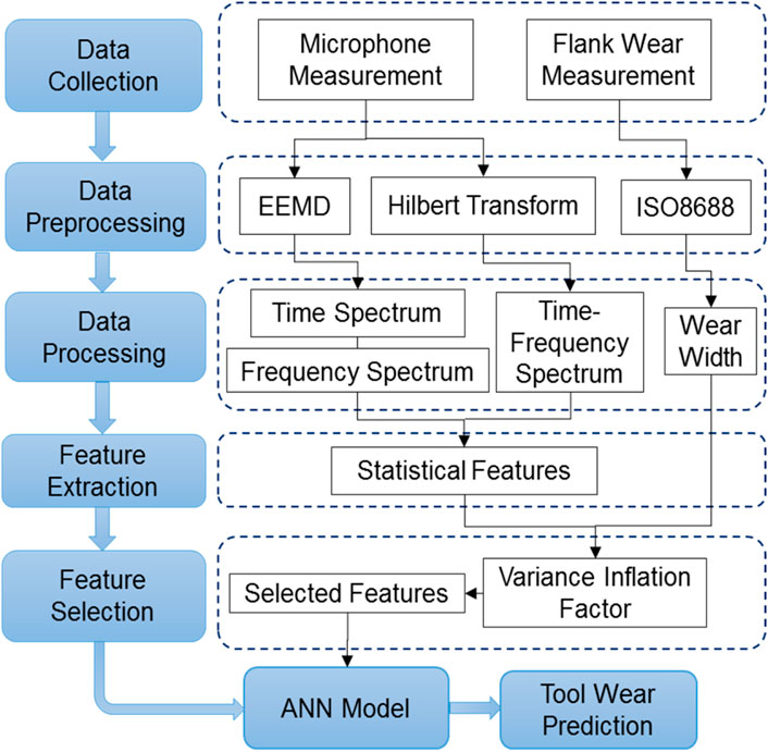
Figure 1. Flow chart of tool wear monitoring.

2.2 Hilbert–huang transform

As mentioned in the literature, HHT is an effective technique for analyzing cutting signals that exhibit nonlinear and non-stationary characteristics. Thus, it is used in this work to analyze cutting sound signals for tool wear monitoring. First, the measured audio signals are decomposed into a set of mono-element called IMF by applying the EEMD, as shown in Equation 1. Each IMF represents a simple oscillatory mode.

$x\left(t\right)={\displaystyle \sum _{j=1}^n}{c}_j\left(t\right)+r_n\left(t\right)(1)$

where $c_j\left(t\right)$ presents the jth intrinsic mode function, which is considered as a mono-element signal, while the residual $r_n\left(t\right)$, as a monotonic function, represents either a constant or the mean trend.

Figure 2 shows the detailed procedure of EEMD, where the shifting process is used to extract the original measured sound signal into several IMFs. The shifting process stops when the residual signal reaches a monotonic function or a constant, and the residual signal could not be further decomposed.

Figure 2

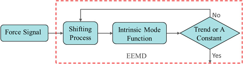
Figure 2. Block diagram of ensemble empirical mode decomposition (EEMD).

Once the EEMD process is completed, the IMFs are extracted. HT is then used to transform each of the disintegrated IMF using Equation 2 below.

$y_j\left(t\right)=H\left[c_j\left(t\right)\right]=\frac{P}{\pi }{\displaystyle \underset{-\infty }{\overset{\infty }{\int }}}\frac{c_j\left(\tau \right)}{t-\tau }d\tau (2)$

in which P presents the Cauchy principal value of the integral, t is the time, and τ is the shift parameter. The analytic signal is constructed using the Hilbert Transform, as defined in Equations 3, 4 below.

$z_j\left(t\right)=c_j\left(t\right)+iH\left[c_j\left(t\right)\right]=A_j{e}^{i{\varphi }_j\left(t\right)}(3)$

$A_j=\sqrt{c_j^2\left(t\right)+y_j^2\left(t\right)}(4)$

where A_j presents the amplitude of instantaneous frequency f_j, which is calculated by Equation 5. It represents the time and frequency domain of the jth IMF, and it can be described in terms of the instantaneous phase angle ϕ_j(t) determined by Equation 6:

$f_j=\frac{1}{2\pi }\frac{d{\varphi }_j\left(t\right)}{dt}(5)$

${\varphi }_j\left(t\right)={\mathit{tan}}^{-1}\left[\frac{y_j\left(t\right)}{c_j\left(t\right)}\right](6)$

The local energy of instantaneous frequency and the mean instantaneous frequency of IMFs are considered as the cutting signal features to estimate the degree of tool wear.

Since instantaneous frequency varies with time, the center frequency f_cj of the jth IMF is defined as the average of the instantaneous frequency over time, weighted by the amplitude (or energy) of the IMF. This is the energy-weighted mean frequency and the center frequency is defined as follow.

$f_{cj}=\frac{\int f_j\left(t\right).A_j^2\left(t\right)dt}{\int A_j^2\left(t\right)dt}(7)$

where A_j is the amplitude of the instantaneous frequency f_j of the jth IMF.

The Hilbert-Huang spectrum, which represents the time–frequency distribution of the amplitude, is then defined by Equation 8 below.

$x\left(t\right)={\displaystyle \sum _{n=1}^N}{A}_n\left(t\right)e^{i\left(\int 2\pi f_n\left(t\right)dt\right)}(8)$

2.3 Feature selection

The feature selection method aims to eliminate the weak and irrelevant features, thereby improving the performance of the proposed prediction model. In this work, multiple statistical features were generated from the dominant IMFs across different domains, including the time domain, frequency domain, and time-frequency domain, which may exhibit strong correlations. Collinearity diagnostics is ussually used to address collinearity or multi-collinearity in feature selection for tool wear prediction, ensuring the reliability and stability of machine learning models. In machining signal analysis, extracted features, such as energy ratios and statistical indicators, often exhibit strong correlations due to their shared physical origins. High multicollinearity among these features can inflate variance in regression coefficients, reduce model interpretability, and lead to overfitting. There have been many feature selection methods proposed to deal with collinearity. Correlation coefficients and mutual information, which rank features based on their relevance to the target variable (Zhou H. et al., 2022). These are often used in the early stages of model development due to their simplicity. Wrapper methods like recursive feature elimination (RFE) provide higher accuracy by evaluating feature subsets through iterative model training, but they are computationally intensive (Bulut et al., 2025). Variance inflation factor (VIF) is a technique that specifically targets multicollinearity among features (Kyriazos and Poga, 2023), which is well-suited to remove highly correlated features in the time domain, frequency domain, and time-frequency domain in this study. The VIF quantifies the degree of multi-collinearity between the self-variable x_i and other independent variables, as described in Equation 9. The tolerance R_xi is determined using Equation 10.

$VIF=\frac{1}{1-R_{xi}^2}(9)$

$R_{x_i}=\frac{{\displaystyle {\sum }_{i,k=1}^n}\left(x_i-{\overline{x}}_i\right)\left(x_k-{\overline{x}}_k\right)}{\sqrt{{\displaystyle {\sum }_{i=1}^n}{\left(x_i-{\overline{x}}_i\right)}^2{\displaystyle {\sum }_{k1}^n}{\left(x_k-{\overline{x}}_k\right)}^2}}(10)$

The VIF for each feature indicates the degree to which the variance of its estimated regression coefficient is inflated due to its correlation with other predictors. Based on widely accepted guidelines (James et al., 2023), VIF values are interpreted as follows:

• VIF = 1: Indicates complete independence (no multicollinearity).

• VIF <5: Suggests low multicollinearity; features are generally safe to retain.

• VIF between 5 and 10: Indicates moderate multicollinearity; may be acceptable depending on the model and context.

• VIF >10: Indicates strong multicollinearity; such features should typically be removed to improve model stability and interpretability.

In this study, any feature with a VIF value greater than 10 was considered to exhibit strong multicollinearity and was eliminated.

2.4 Artificial neural network

Once the important features are identified, they serve as the inputs to an artificial neural network (ANN) model for estimating tool wear. By learning from the training data, the ANN model offers the advantage of mapping signal features to flank wear (Ghosh et al., 2007). An ANN consists of interconnected nodes called neurons, and is a strong candidate for solving classification problems. Particularly, ANNs are well suited for handling complex decision boundary problems involving multiple variables. A single neuron in the ANN model, which represents the relationship between inputs and outputs, is described in Equations 11, 12.

${\widehat{y}}_i=f\left[{\displaystyle \sum _{i=1}^n}{w}_i*x_i-\theta \right](11)$

$f\left(x\right)=\frac{1}{1+e^{-x}}(12)$

where w_i describes the weight between neurons, θ presents the threshold, and f(x) represents the sigmoid function.

The Back-propagation Neural Network (BPNN), which consists of a forward pass and a backward pass, is a multi-layer network with excellent learning capabilities. In this process, the backward pass aims to use the last objective function (loss/cost function) to update the parameters (Asiltürk and Cunkas, 2011). Typically, the mean square error (MSE), described in Equation 13, is used as the objective function. If the error value is large, it indicates that the model parameters are not well learned. In such cases, training must continue until the parameters or error values converge.

$MSE=\frac{1}{n}\sum _{i=1}^m{\left(y_i-{\widehat{y}}_i\right)}^2(13)$

This study used the Levenberg-Marquardt algorithm to optimize the internal structure of the nonlinear multi-layer network and update the weights and bias values in the ANN model. This training method offers the advantages of fast convergence, and is suitable for small to medium-sized datasets (Bano et al., 2024). The weights of the training model in this study were optimized and updated according to Equations 14–16.

$w_{k+1}=w_k-{\left(J^{T}J+\mu I\right)}^{-1}{J}^T\mathrm{e}(14)$

where μ is the adaptive damping factor adjusted depending on the weight error, I is identify matrix, e is the error calculated during the forward pass and is backpropagated to the previous layers to update their weights, J is Jacobian matrix calculated during the backward pass.

$e_i={\mathrm{y}}_i-{\widehat{y}}_i(15)$

$J_{ij}=\frac{\partial e_i}{\partial w_i}(16)$

The biases were also optimized and updated in the same way and alongside the weights using Levenberg-Marquardt algorithm. The structure of the proposed ANN model optimized using the Levenberg–Marquardt algorithm consists of eight input nodes, a hidden layer with twelve nodes, and a single output node. To ensure stable and efficient training, an initial damping rate of 0.01 was selected and adjusted by factors of 10 and 0.1 based on the loss. The data set has been randomly divided into training and testing datasets, with 70% used for training and the remaining 30% for testing.

3 Experimental setup and measurement

To conduct the tool wear experiments, a 3-axis precision milling machine (M350-CNCMTT) with a maximum spindle speed of 24,000 rpm was used in this paper.

A 2-flutes HSS-Cobalt end mill cutter with a diameter of 6 mm was used in all experiments to machine a block of S45C, which was made by casting. The cutting tool and dimensions of the workpiece are illustrated in Figures 3a,b, respectively. The details of the experimental setup are shown in Figure 4.

Figure 3

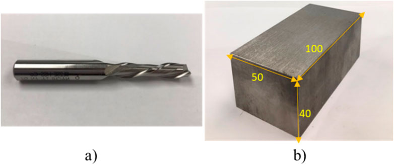
Figure 3. (a) HSS milling cutter and (b) workpiece.

Figure 4

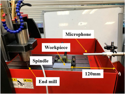
Figure 4. Setup in a three-axis precision milling machine.

The audio signals were collected using an ECM-800 microphone, which has a bandwidth of 15 Hz–20 kHz. A data acquisition module (model NI-9234) was used to transmit the collected data at a sampling rate of 51.2k samples/sec. As shown in Figure 4, the microphone was fixed to the CNC machine using magnetic attraction, with its receiving end positioned close to the cutting region. A two-dimensional image measurement instrument (model of EVM-2515) was used to record the degree of tool wear after each cut.

In this research, nine down-milling experiments were conducted under dry cutting conditions. All experiments were performed in the stable cutting environment, where the cutting depth was 0.5 mm and the cutting width was 2.5 mm. The cutting conditions for the tool wear experiment, including various spindle speeds and feed rates, are listed in Table 1. The cutting distance per cut was 103 mm. After each cut, the flank wear was measured until the end of the tool life. The international standard ISO 8688 was used to determine the tool life (ISO, 1989).

Table 1

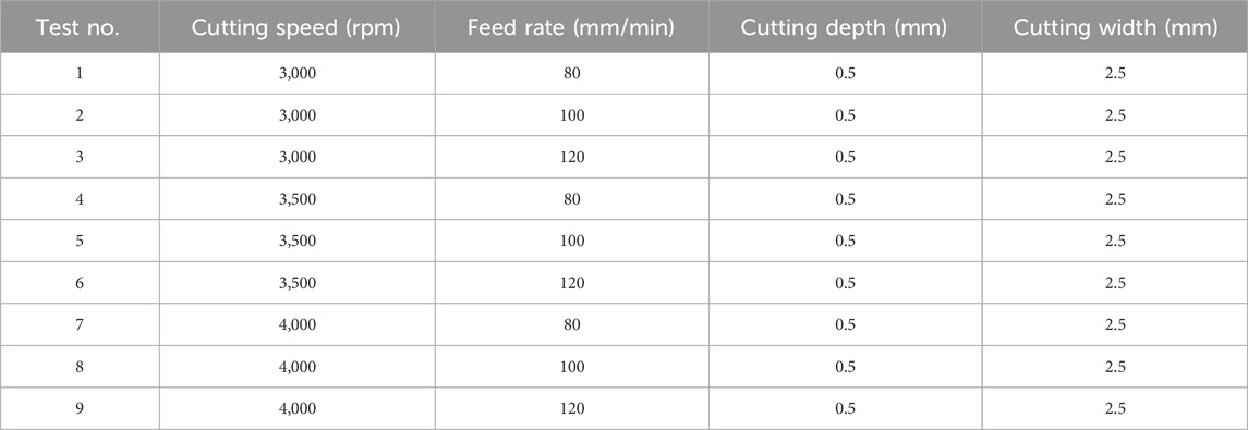
Table 1. Tool wear experiment under various cutting conditions.

A LabVIEW program was developed to capture audio signals during machining. The LabVIEW interface and the corresponding tool wear under the cutting condition of 4,000 rpm and 100 mm/min are shown in Figure 5. The tool wear progression for each cutting tool was captured using the EVM-2515 instrument and is illustrated in Figure 6.

Figure 5

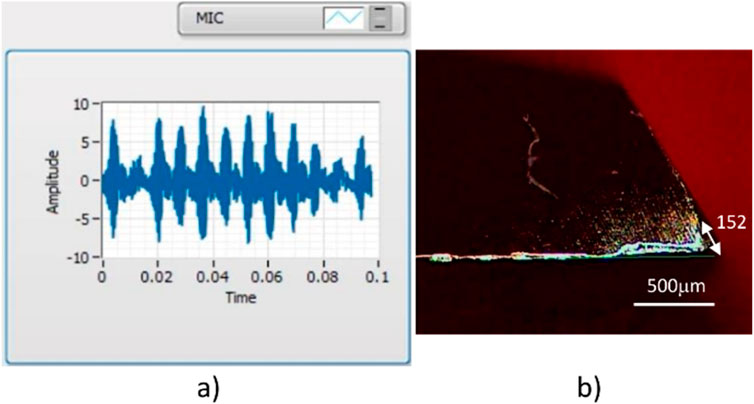
Figure 5. (a) LabVIEW Interface and (b) flank wear measurement.

Figure 6

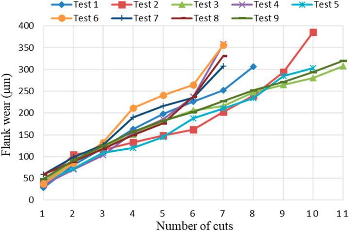
Figure 6. Measured flank wear curves under various cutting conditions.

4 Analysis results and discussions

The measured audio signals were decomposed into eight Intrinsic Mode Functions (IMFs) using Ensemble Empirical Mode Decomposition (EEMD), as described in Equation 1. Figure 7 shows the first eight IMFs obtained from the worn audio signal recorded at a spindle speed of 3,000 rpm and a feed rate of 80 mm/min. Subsequently, the Hilbert Transform (HT) was applied to each IMF. To evaluate the significance of each IMF, their energy ratios were computed according to Equation 17, with the results presented in Figure 8.

$r_j=\frac{{\displaystyle {\int }_{-\infty }^{+\infty }}{\left|c_j\left(\omega \right)\right|}^{2}d\omega }{{\displaystyle {\int }_{-\infty }^{+\infty }}{\left|x\left(\omega \right)\right|}^{2}d\omega }(17)$

where, $r_j$ is the energy ratio of the jth IMF, $c_j\left(\omega \right)$ is spectral representation of the jth IMF, $x\left(\omega \right)$ is spectral representation of the original signal, ${\left|c_j\left(\omega \right)\right|}^2$ is spectral energy density of the IMF, ${\left|x\left(\omega \right)\right|}^2$ is spectral energy density of the full signal.

Figure 7

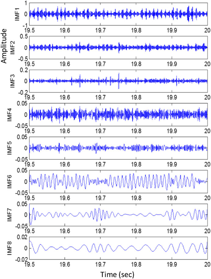
Figure 7. The results of the first eight IMFs of the cutting sound signals.

Figure 8

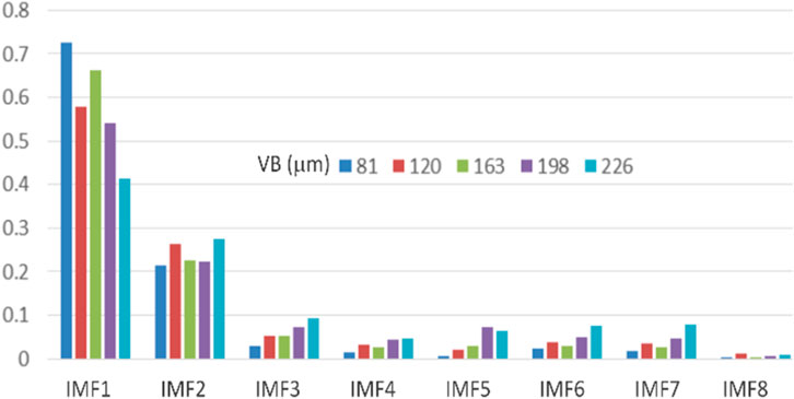
Figure 8. The energy ratio of the first eight IMFs.

Among all IMFs, IMF1 consistently exhibited the highest energy ratio across all tool wear conditions, indicating that it captures well the primary vibration components related to the cutting process.

Additionally, the center frequencies of IMF1, calculated using Equation 7, are summarized in Table 2, clearly showing that these frequencies lie within the energy bandwidth range of 6,100 Hz–6,500 Hz. To validate the mechanical relevance of this frequency range, a sweeping test was performed by gradually increasing the spindle speed under non-cutting conditions to identify the resonant frequencies of the tool–spindle holder. The recorded sound signals from this test were transformed into a frequency spectrum using the Fast Fourier Transform (FFT), generating the 3D multiplot frequency spectrum presented in Figure 9. It was observed that the center frequencies of IMF1 (6,100–6,500 Hz) closely overlapped with the machine’s structural resonant frequency.

Table 2

Table 2. Center frequencies, defined by Equation 7, of IMF1 of Test No. 1.

Figure 9

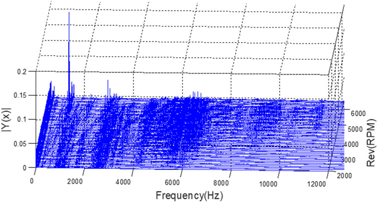
Figure 9. 3D multi-plot frequency spectrum obtained from under non-cutting conditions.

The overlap between IMF1’s center frequencies and the machine’s resonant frequency is particularly significant because signals near the structural resonance are typically amplified and highly sensitive to changes in mechanical conditions like tool wear, chatter, or other dynamic instabilities. This frequency alignment ensures that IMF1 reliably captures the mechanical interactions and vibration behaviors directly linked to the cutting process. Therefore, IMF1 was selected for extracting statistical features that characterize the local properties the signal, such as peaks, symmetry, and spread, in both the time domain and time–frequency domain. In addition, the energy ratios of all IMFs (r_IMF1 to r_IMF8 were used as energy-based features, capturing the global energy distribution of the signal across frequency bands in the frequency domain. In this study, various statistical features were generated from the IMF1 in time domain and time-frequency domain. These features are the most common used in signal-based tool wear monitoring, which include kurtosis (KU), skewness (SK), standard deviation (SD), root mean square (RMS), maximum value (MAX), variance (VAR), mean (ME), and crest factor (CF) (Abubakr et al., 2021; Lara de Leon et al., 2024; Mohamed et al., 2022). KU measures the tailedness of the signal distribution. A high KU implies more extreme values or spikes in the signal, indicating sudden impacts from tool chipping or cracking, often caused by worn tools. SK measures the asymmetry of the signal’s amplitude distribution. Changes in SK reflect misalignment or material accumulation on one side of the tool, indicating asymmetric wear. SD quantifies the spread of signal values around the mean. A high SD indicates increased vibration variability or cutting force fluctuations due to tool wear or chipping. RMS measures the effective amplitude or power content of a signal. An increase in RMS reflects greater energy from friction and rubbing, implying progressing tool wear. MAX is the highest amplitude observed in the signal. Spikes in MAX are signs of sudden impact events, which may occur due to severely worn or damaged tools. VAR is the square of SD, representing the signal’s dispersion. A higher VAR indicates greater signal variability due to intensified tool material interactions as wear progresses. ME is the arithmetic average of all signal values. Shifts in ME reflect changes in the baseline force or vibration level, typically associated with progressive tool wear. CF is the ratio of peak amplitude to RMS. A high CF suggests localized, sudden signal events amid steady cutting, such as severe wear or the initiation of cracks. All of these statistical features extracted from IMF1 were calculated and are presented in Table 3. Moreover, the energy-based features for all IMFs were computed using Equation 17. As a result, a total of 22 features were generated across the time domain, frequency domain, and time–frequency domain, as detailed in Table 4.

Table 3

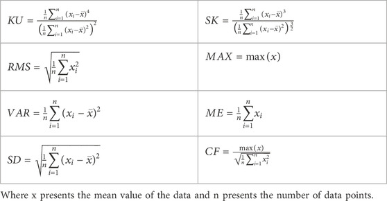
Table 3. The statistical features.

Table 4

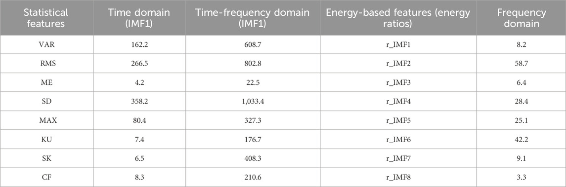
Table 4. Extracted statistical and energy-based features from multiple signal domains.

To improve the performance and reliability of the developed tool wear monitoring system, it is essential to eliminate irrelevant and redundant features from the extracted feature set. A key issue that negatively impacts model accuracy is multicollinearity, which occurs when two or more features are highly linearly correlated. To address this, the VIF was employed as a quantitative measure of multicollinearity among features. In this study, VIF values were computed using Equations 9, 10, and any feature with a VIF greater than 10 was considered to exhibit serious multicollinearity. These features were excluded to prevent model instability, inflated standard errors, and reduced clarity in interpreting feature importance. By applying this threshold, eight features with acceptable VIF values (≤10) were selected for the final analysis, as presented in Table 5. This subset includes four time-domain features extracted from IMF1 and four energy-ratio features representing the energy distribution across selected IMFs in the frequency domain.

Table 5

Table 5. Selected wear features based on the VIF criterion.

Once the feature selection procedure was completed, the selected featured were fed into the ANN model to predict tool wear. In the developed system, the ANN model used Levenberg-Marquardt optimization with eight input nodes, twelve hidden nodes, and one output node. The data set has been randomly divided into training and testing datasets, with 70% used for training and the remaining 30% for testing. Figure 10 presents the results of tool wear prediction using the ANN model with feature selection (ANN + FS) and without feature selection (ANN) under multiple cutting conditions. The results indicate that the ANN model without feature selection performed the worst. However, the prediction accuracy was significantly improved when feature selection was applied. Their performances are compared and presented in Table 6. The prediction accuracy of the developed method aligns well with the measured tool wear across different cutting conditions, with an average prediction accuracy of approximately 90.03%.

Figure 10

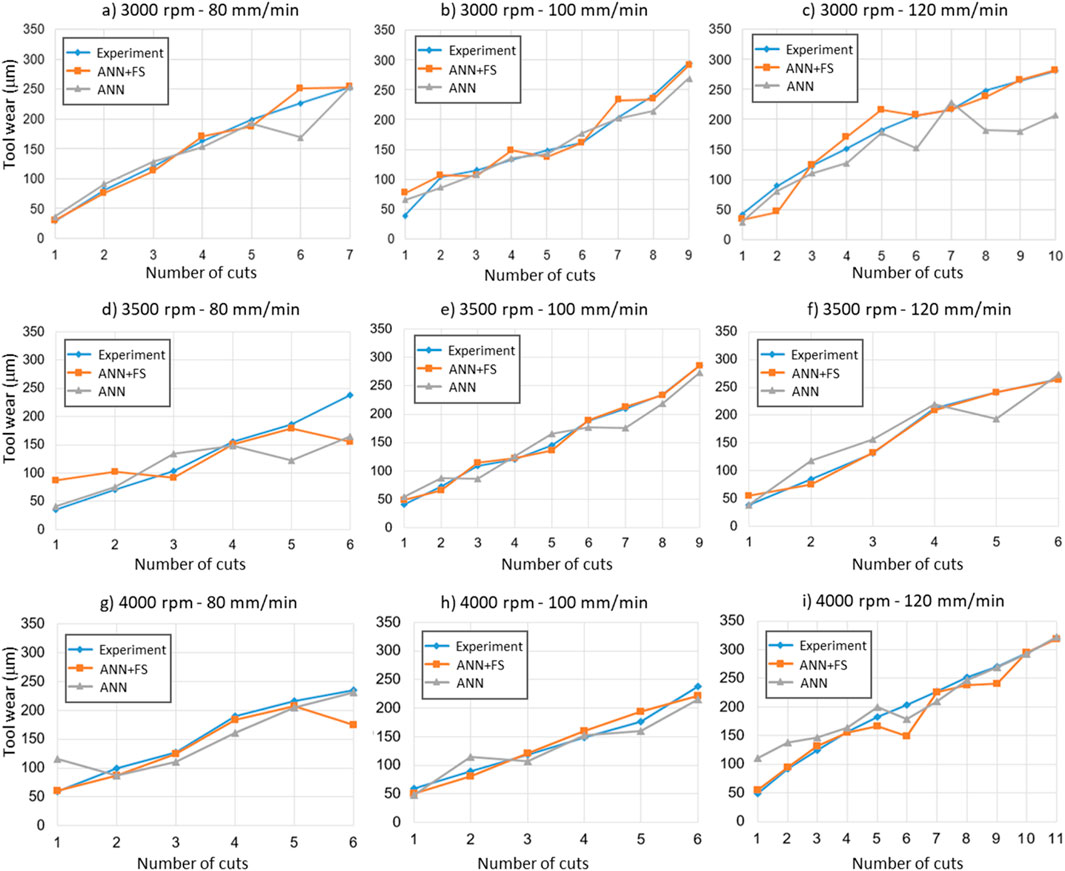
Figure 10. Tool wear prediction across various cutting conditions: (a) 3000 rpm – 80 mm/min, (b) 3000 rpm – 100 mm/min, (c) 3000 rpm – 120 mm/min, (d) 3500 rpm – 80 mm/min, (e) 3500 rpm – 100 mm/min, (f) 3500 rpm – 120 mm/min, (g) 4000 rpm – 80 mm/min, (h) 4000 rpm – 100 mm/min, (i) 4000 rpm – 120 mm/min.

Table 6

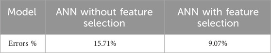
Table 6. Comparison of prediction errors.

The significant improvement in tool wear prediction when feature selection is applied in this study highlights the critical importance of preprocessing raw audible sound signals and selecting the most informative and meaningful features for input into the ANN machine learning model. Machining environments often introduce various noise sources unrelated to the cutting process, such as coolant sprays or sounds from other machine components, which can introduce irrelevant features that degrade model performance and reliability. Furthermore, tool wear generates complex, nonlinear, and nonstationary sound signals with time-varying frequency content. In this study, signal preprocessing using Ensemble Empirical Mode Decomposition (EEMD) and the Hilbert Transform effectively isolated meaningful signal components and extracted features that accurately reflect tool wear, rather than environmental interference. This process yielded relevant features across multiple domains (time, frequency, and time-frequency domains). However, these features may exhibit multicollinearity, which can lead to overfitting and model instability. Therefore, a Variance Inflation Factor (VIF)-based feature selection technique was further employed in this study to identify and remove highly correlated features to stablize and improve the prediction accuracy from 84.29% (ANN without FS) to 90.03% (ANN with FS).

In Ref. (Kothuru et al., 2017), the authors so emphasize the critical importance of applying preprocessing techniques to extract physical parameters that closely correlate with actual tool wear. In their study, audible sound signals were transformed into the frequency domain using the Short-Time Fourier Transform (STFT). From this transformation, the amplitudes at each data point and their average values were extracted as features. These features were then used as inputs to a Support Vector Machine (SVM) model for predicting tool wear conditions. The prediction accuracy achieved ranged from 85.3% to 98.5%, depending on the wear class. The authors concluded that the lower accuracy observed in certain wear classes may be attributed to the limitations of the applied preprocessing methods, which may not have been sufficient to filter out noise. Consequently, they suggested that more effective preprocessing techniques with feature selection are necessary to enhance signal quality and improve prediction performance. Similarly, (Li et al., 2019), demonstrated the effectiveness of advanced signal processing and feature selection techniques in enhancing the prediction accuracy of machine learning models for tool wear. In their study, the authors applied Extended Convolutive Bounded Component Analysis (ECBCA) to separate source audible sound signals from wavelet sub-band signals obtained during milling tests. The separated source signals were then further denoised using a Multivariate Synchrosqueezing Transform (MSST), which decomposed them into time-varying oscillatory components. Several statistical features were subsequently extracted from the time-frequency domain and used as inputs to various machine learning models, including Classification and Regression Tree (CART), Random Forest (RF), k-Nearest Neighbors (KNN), and Support Vector Machine (SVM), to predict tool wear conditions. The results showed that without ECBCA preprocessing, the prediction accuracy ranged from 83.34% to 98.19%, depending on the wear class and the chosen model. With the employment of ECBCA, the accuracy improved further, reaching a range of 86.14%–100%, thereby underscoring the importance of effective signal preprocessing for accurate and robust tool wear prediction. While these studies consistently report high prediction accuracies when effective preprocessing and feature selection techniques are used, the actual performance varies across studies due to differences in data processing, feature selection methods, and machine learning models. For instance, (Ravikumar and Ramachandran, 2018), evaluated tool wear prediction using a decision tree J48 model with different input feature sets: basic statistical features (e.g., mean, kurtosis, standard deviation, variance, and maximum), Haar wavelet energy features, and a small subset of those energy features. Their results showed that statistical features yielded the lowest accuracy (82.41%), while full Haar wavelet energy features and the selected subset produced higher accuracies of 93.15% and 93.7%, respectively. In the work of (Li et al., 2019), using the same data preprocessing and feature extraction methods, SVM consistently outperformed CART, RF, and KNN. Similarly, (Catalán et al., 2022), demonstrated the strong potential of deep learning using a VGG16 neural network architecture for accurate tool wear prediction. Moreover, external factors such as the microphone placement during sound signal acquisition can significantly impact prediction performance. (Kothuru et al., 2018). investigated the effect of microphone positioning by conducting experiments with multiple microphones placed at varying distances from the cutting zone. The resulting sound features were used with an SVM model, yielding prediction accuracies ranging from 89.1% to 97% depending on microphone location. Interestingly, the dataset collected from the farthest microphone achieved higher accuracy, likely due to reduced noise interference and fewer obstructions between the microphone and cutting zone.

From the above discussion, it is evident that although the prediction accuracies reported across different sound-based tool wear monitoring studies vary due to factors such as data acquisition setup, feature selection strategies, and machine learning model choices, substantial improvements can be consistently achieved through the application of robust signal preprocessing and advanced feature selection techniques. The approach proposed in this study, combining EEMD, Hilbert Transform, and VIF-based feature selection, demonstrates strong potential for practical implementation in real-time tool condition monitoring systems.

5 Conclusion

Tool wear monitoring is essential for improving productivity and preventing severe wear or tool breakage. Most previous studies on the tool wear monitoring used signals measured by various sensors, such as dynamometers, accelerometers, and AE sensors. However, these sensors are challenging to use in manufacturing environments due to their high costs and complex installation requirements. In contrast, microphones offer a cost-effective alternative for practical tool wear monitoring applications. This paper proposed a novel approach to indirect online tool wear monitoring in the milling process by investigating the correlation between audio signals and cutting tool wear. The measured data signals were analyzed using EEMD and HT, allowing tool wear features to be generated from the time domain, frequency spectrum, and time-frequency domain. Since the performance of the tool wear monitoring system was affected by weak wear features, the multi-collinearity between features was evaluated using the VIF tests to determine the significant features that can improve the wear prediction accuracy. An ANN model was developed to learn the wear features from the datasets to estimate the degree of tool wear. The proposed tool wear prediction method, which integrates the ANN model with feature selection, achieved high prediction accuracy, exceeding 90% on average under various cutting conditions. The study also highlighted that, although various machine learning models can be employed and may yield high prediction accuracy, effective data preprocessing and feature selection remain the most critical factors for achieving reliable, meaningful, and accurate results, particularly in audible sound signal-based tool wear condition monitoring systems. The proposed approach demonstrates strong potential for practical implementation and offers a low-cost, efficient solution for real-time tool wear monitoring in manufacturing environments.

Data availability statement

The raw data supporting the conclusions of this article will be made available by the authors, without undue reservation.

Author contributions

VV: Conceptualization, Formal Analysis, Investigation, Methodology, Software, Supervision, Validation, Writing – original draft, Writing – review and editing. T-NB: Data curation, Methodology, Writing – review and editing. M-QT: Conceptualization, Formal Analysis, Investigation, Methodology, Project administration, Resources, Software, Supervision, Validation, Writing – review and editing.

Funding

The author(s) declare that financial support was received for the research and/or publication of this article. This research was funded by Thai Nguyen University of Technology (TNUT) under project grant number T2024-TS26.

Acknowledgments

The authors thank Thai Nguyen University of Technology (TNUT), Vietnam, for the support.

Conflict of interest

The authors declare that the research was conducted in the absence of any commercial or financial relationships that could be construed as a potential conflict of interest.

Generative AI statement

The author(s) declare that no Generative AI was used in the creation of this manuscript.

Publisher’s note

All claims expressed in this article are solely those of the authors and do not necessarily represent those of their affiliated organizations, or those of the publisher, the editors and the reviewers. Any product that may be evaluated in this article, or claim that may be made by its manufacturer, is not guaranteed or endorsed by the publisher.

References

Abubakr, M., Hassan, M. A., Krolczyk, G. M., Khanna, N., and Hegab, H. (2021). Sensors selection for tool failure detection during machining processes: a simple accurate classification model. CIRP J. Manuf. Sci. Technol. 32, 108–119. doi:10.1016/j.cirpj.2020.12.002

CrossRef Full Text | Google Scholar

Akkoyun, F., Ercetin, A., Aslantas, K., Pimenov, D. Y., Giasin, K., Lakshmikanthan, A., et al. (2021). Measurement of micro burr and slot widths through image processing: comparison of manual and automated measurements in micro-milling. Sensors 21 (13), 4432. doi:10.3390/s21134432

PubMed Abstract | CrossRef Full Text | Google Scholar

Alphonse, M., Raja, V. K. B., Cepova, L., Salunkhe, S., Nasr, E. A., and Abdelgawad, A. E. (2024). Tribological and investigation study of a dlc-coated H13 friction drilling tool on AZ31B magnesium alloy. Front. Mech. Eng. 10. doi:10.3389/fmech.2024.1470507

CrossRef Full Text | Google Scholar

Anas, N. M., Yusof, M. Y. M., and Aziz, M. Z. A. (2022). “Machine tool condition monitoring system: a review on feasible solution,” in Paper presented at the 2022 International Conference on Artificial Intelligence of Things (ICAIoT), Istanbul, Turkey, 29-30 December 2022 (IEEE).

CrossRef Full Text | Google Scholar

Antsev, A. V., Zhmurin, V. V., Yanov, E. S., and Dang, T. H. (2019). Cutting tool wear monitoring using the diagnostic capabilities of modern CNC machines. J. Phys. Conf. Ser. 1260 (3), 032003. doi:10.1088/1742-6596/1260/3/032003

CrossRef Full Text | Google Scholar

Asiltürk, I., and Cunkas, M. (2011). Modeling and prediction of surface roughness in turning operations using artificial neural network and multiple regression method. Expert Syst. Appl. 38, 5826–5832. doi:10.1016/j.eswa.2010.11.041

CrossRef Full Text | Google Scholar

Bagga, P. J., Chavda, B., Modi, V., Makhesana, M. A., and Patel, K. M. (2022). Indirect tool wear measurement and prediction using multi-sensor data fusion and neural network during machining. Mater. Today Proc. 56, 51–55. doi:10.1016/j.matpr.2021.12.131

CrossRef Full Text | Google Scholar

Bano, F. H., Ali, R., Mohammad, S., Faraz, H., and Khalifa, H. S. (2024). An artificial neural network and levenberg-marquardt training algorithm-based mathematical model for performance prediction. Appl. Math. Sci. Eng. 32 (1), 2375529. doi:10.1080/27690911.2024.2375529

CrossRef Full Text | Google Scholar

Buggineni, V., Chen, C., and Camelio, J. (2024). Enhancing manufacturing operations with synthetic data: a systematic framework for data generation, accuracy, and utility. Front. Manuf. Technol. 4. doi:10.3389/fmtec.2024.1320166

CrossRef Full Text | Google Scholar

Bulut, O., Tan, B., Mazzullo, E., and Syed, A. (2025). Benchmarking variants of recursive feature elimination: insights from predictive tasks in education and healthcare. Preprints.

Google Scholar

Catalán, C., Canales, H., Cruz-González, C., and Torres, M. (2022). Cutting tool wear monitoring through cutting sound classification and machine learning.

Google Scholar

Chen, X., and Li, B. (2007). Acoustic emission method for tool condition monitoring based on wavelet analysis. Int. J. Adv. Manuf. Technol. 33 (9), 968–976. doi:10.1007/s00170-006-0523-5

CrossRef Full Text | Google Scholar

Chen, C.-H., and Lin, C.-J. (2022). Using neural networks for tool wear prediction in computer numerical control end milling. Sensors Mater. 34, 803. doi:10.18494/sam3642

CrossRef Full Text | Google Scholar

Dosko, S. I., Sheptunov, S. A., Ryad, A., and Rudnev, S. K. (2023). “Application of empirical mode decomposition to reduce signal noise,” in International Conference on Quality Management, Transport and Information Security, Information Technologies (IT&QM&IS), Petrozavodsk, Russian Federation, 25-29 Sept. 2023 (IEEE).

CrossRef Full Text | Google Scholar

Gasca, M. V., Bueno-Lopez, M., Molinas, M., and Fosso, O. B. (2018). Time-frequency analysis for nonlinear and non-stationary signals using HHT: a mode mixing separation technique. IEEE Lat. Am. Trans. 16 (4), 1091–1098. doi:10.1109/tla.2018.8362142

CrossRef Full Text | Google Scholar

Ghosh, N., Ravi, Y. B., Patra, A., Mukhopadhyay, S., Paul, S., Mohanty, A. R., et al. (2007). Estimation of tool wear during CNC milling using neural network-based sensor fusion. Mech. Syst. Signal Process. 21, 466–479. doi:10.1016/j.ymssp.2005.10.010

CrossRef Full Text | Google Scholar

Heitz, T., Bachrathy, D., He, N., Chen, N., and Stepan, G. (2023). Optimization of cutting force fitting model by fast fourier transformation in milling. J. Manuf. Process. 99, 121–137. doi:10.1016/j.jmapro.2023.05.046

CrossRef Full Text | Google Scholar

Hong, Y.-S., Yoon, H.-S., Moon, J.-S., Cho, Y.-M., and Ahn, S.-H. (2016). Tool-wear monitoring during micro-end milling using wavelet packet transform and Fisher’s linear discriminant. Int. J. Precis. Eng. Manuf. 17 (7), 845–855. doi:10.1007/s12541-016-0103-z

CrossRef Full Text | Google Scholar

Hundt, W., Leuenberger, D., Rehsteiner, F., and Gygax, P. (1994). An approach to monitoring of the grinding process using acoustic emission (AE) technique. CIRP Ann. 43 (1), 295–298. doi:10.1016/s0007-8506(07)62217-3

CrossRef Full Text | Google Scholar

Imad, M., Hopkins, C., Hosseini, Icon, A., Hosseini, A., Yussefian, N. Z., and Kishawy, H. A. (2022). Intelligent machining: a review of trends, achievements and current progress. Int. J. Comput. Integr. Manuf. 35 (4-5), 359–387. doi:10.1080/0951192x.2021.1891573

CrossRef Full Text | Google Scholar

ISO (1989). Tool life testing in milling, part 2: end milling.

Google Scholar

James, G., Witten, D., Hastie, T., Tibshirani, R., and Taylor, J. (2023). An introduction to statistical learning. Cham: Springer.

Google Scholar

Jemielniak, K. (2010). Tool wear monitoring based on wavelet transform of raw acoustic emission signal. Adv. Manuf. Sci. And Technol. 34, 5–17.

Google Scholar

Jirapipattanaporn, P., Chanpariyavatevong, A., Lawanont, W., and Boongsood, W. (2023). Tool wear analysis on time-domain and frequency-domain data of machining S45C using signal processing technique, 69–77.

Google Scholar

Kaliyannan, D., Thangamuthu, M., Pradeep, P., Gnansekaran, S., Rakkiyannan, J., and Pramanik, A. (2024). Tool condition monitoring in the milling process using deep learning and reinforcement learning. J. Sens. Actuator Netw. 13 (4), 42. doi:10.3390/jsan13040042

CrossRef Full Text | Google Scholar

Kang, G.-S., Kim, S.-G., Yang, G.-D., Park, K.-H., and Lee, D. Y. (2019). Tool chipping detection using peak period of spindle vibration during end-milling of inconel 718. Int. J. Precis. Eng. Manuf. 20 (11), 1851–1859. doi:10.1007/s12541-019-00241-7

CrossRef Full Text | Google Scholar

Kasiviswanathan, S., Gnanasekaran, S., Thangamuthu, M., and Rakkiyannan, J. (2024). Machine-Learning- and internet-of-things-driven techniques for monitoring tool wear in machining process: a comprehensive review. J. Sens. Actuator Netw. 13 (5), 53. doi:10.3390/jsan13050053

CrossRef Full Text | Google Scholar

Katamba Mpoyi, D., Ekuakille, A. L., Ugwiri, M. A., Casavola, C., and Pappalettera, G. (2024). Wear monitoring based on vibration measurement during machining: an application of FDM and EMD. Meas. Sensors 32, 101051. doi:10.1016/j.measen.2024.101051

CrossRef Full Text | Google Scholar

Kon, T., Mano, H., Iwai, H., Ando, Y., Korenaga, A., Ohana, T., et al. (2024). Effect of acoustic emission sensor location on the detection of grinding wheel deterioration in cylindrical grinding. Lubricants 12 (3), 100. doi:10.3390/lubricants12030100

CrossRef Full Text | Google Scholar

Kothuru, A., Nooka, S. P., Iglesias Victoria, P., and Liu, R. (2017). “Application of audible sound signals for tool wear monitoring and workpiece hardness identification in gear milling using machine learning techniques,” in Paper presented at the ASME 2017 International Design Engineering Technical Conferences and Computers and Information in Engineering Conference, Cleveland, Ohio, USA, November 3, 2017.

Google Scholar

Kothuru, A., Nooka, S. P., and Liu, R. (2018). Application of audible sound signals for tool wear monitoring using machine learning techniques in end milling. Int. J. Adv. Manuf. Technol. 95 (9), 3797–3808. doi:10.1007/s00170-017-1460-1

CrossRef Full Text | Google Scholar

Kyriazos, T., and Poga, M. (2023). Dealing with multicollinearity in factor analysis: the problem, detections, and solutions. Open J. Statistics 13, 404–424. doi:10.4236/ojs.2023.133020

CrossRef Full Text | Google Scholar

Lara de Leon, M. A., Kolarik, J., Byrtus, R., Koziorek, J., Zmij, P., and Martinek, R. (2024). Tool condition monitoring methods applicable in the metalworking process. Archives Comput. Methods Eng. 31 (1), 221–242. doi:10.1007/s11831-023-09979-w

CrossRef Full Text | Google Scholar

Li, Z., Liu, R., and Wu, D. (2019). Data-driven smart manufacturing: tool wear monitoring with audio signals and machine learning. J. Manuf. Process. 48, 66–76. doi:10.1016/j.jmapro.2019.10.020

CrossRef Full Text | Google Scholar

Li, G., Shang, X., Sun, L., Fu, B., Yang, L., and Zhou, H. (2025). Application of audible sound signals in tool wear monitoring: a review. J. Adv. Manuf. Sci. Technol. 5 (1), 0. doi:10.51393/j.jamst.2025003

CrossRef Full Text | Google Scholar

Liu, G., Huang, C., Wang, X., Zhao, B., and Ji, M. (2024). Friction and wear of cutting tools and cutting tool materials. Lubricants 12 (6), 192. doi:10.3390/lubricants12060192

CrossRef Full Text | Google Scholar

Liu, Z., Lang, Z.-Q., Gui, Y., Zhu, Y.-P., and Laalej, H. (2024). Digital twin-based anomaly detection for real-time tool condition monitoring in machining. J. Manuf. Syst. 75, 163–173. doi:10.1016/j.jmsy.2024.06.004

CrossRef Full Text | Google Scholar

Maia, L. H. A., Abrão, A. M., Vasconcelos, W. L., Júnior, J. L., Fernandes, G. H. N., and Machado, Á. R. (2024). Enhancing machining efficiency: real-time monitoring of tool wear with acoustic emission and STFT techniques. Lubricants 12 (11), 380. doi:10.3390/lubricants12110380

CrossRef Full Text | Google Scholar

Mamedov, A., Dinc, A., Guler, M. A., Demiral, M., and Otkur, M. (2025). Tool wear in micromilling: a review. Int. J. Adv. Manuf. Technol. 137 (1), 47–65. doi:10.1007/s00170-025-15219-1

CrossRef Full Text | Google Scholar

Mohamed, A., Hassan, M., M’Saoubi, R., and Attia, H. (2022). Tool condition monitoring for high-performance machining systems—A review. Sensors 22 (6), 2206. doi:10.3390/s22062206

PubMed Abstract | CrossRef Full Text | Google Scholar

Mourtzis, D., Vlachou, E., Milas, N., Tapoglou, N., and Mehnen, J. (2019). A cloud-based, knowledge-enriched framework for increasing machining efficiency based on machine tool monitoring. Proc. Institution Mech. Eng. Part B 233 (1), 278–292. doi:10.1177/0954405417716727

CrossRef Full Text | Google Scholar

Navarro-Devia, J. H., Chen, Y., Dao, D. V., and Li, H. (2023). Chatter detection in milling Processes—A review on signal processing and condition classification. Int. J. Adv. Manuf. Technol. 125 (9), 3943–3980. doi:10.1007/s00170-023-10969-2

CrossRef Full Text | Google Scholar

Olalere, I. O., and Olanrewaju, O. A. (2023). Tool and workpiece condition classification using empirical mode decomposition (EMD) with hilbert–huang transform (HHT) of vibration signals and machine learning models. Appl. Sci. 13 (4), 2248. doi:10.3390/app13042248

CrossRef Full Text | Google Scholar

Pai, P. S., and Rao, P. K. R. (2002). Acoustic emission analysis for tool wear monitoring in face milling. Int. J. Prod. Res. 40 (5), 1081–1093. doi:10.1080/00207540110107534

CrossRef Full Text | Google Scholar

Pimenov, D. Y., Bustillo, A., Wojciechowski, S., Sharma, V. S., Gupta, M. K., and Kuntoğlu, M. (2023). Artificial intelligence systems for tool condition monitoring in machining: analysis and critical review. J. Intelligent Manuf. 34 (5), 2079–2121. doi:10.1007/s10845-022-01923-2

CrossRef Full Text | Google Scholar

Ravikumar, S., and Ramachandran, K. I. (2018). Tool wear monitoring of multipoint cutting tool using sound signal features signals with machine learning techniques. Mater. Today Proc. 5 (11), 25720–25729. doi:10.1016/j.matpr.2018.11.014

CrossRef Full Text | Google Scholar

Rehman, A. U., Nishat, T. S. R., Ahmed, M. U., Begum, S., and Ranjan, A. (2024). Chip analysis for tool wear monitoring in machining: a deep learning approach. IEEE Access 12, 112672–112689. doi:10.1109/access.2024.3443517

CrossRef Full Text | Google Scholar

Rmili, W., Serra, R., Ouahabi, A., Gontier, C., and Mecheri, K. (2006). “Tool wear monitoring in turning process using vibration measurement,” in 13th International Congress on Sound and Vibration, Vienna, Austria.

Google Scholar

Rudel, V., Kienast, P., Vinogradov, G., Ganser, P., and Bergs, T. (2022). Cloud-based process design in a digital twin framework with integrated and coupled technology models for blisk milling. Front. Manuf. Technol. 2. doi:10.3389/fmtec.2022.1021029

CrossRef Full Text | Google Scholar

Sánchez Hernández, Y., Trujillo Vilches, F. J., Bermudo Gamboa, C., and Sevilla Hurtado, L. (2019). Online tool wear monitoring by the analysis of cutting forces in transient state for dry machining of Ti6Al4V alloy. Metals 9 (9), 1014. doi:10.3390/met9091014

CrossRef Full Text | Google Scholar

Schueller, A., and Saldaña, C. (2022). Indirect tool condition monitoring using ensemble machine learning techniques. J. Manuf. Sci. Eng. 145 (1). doi:10.1115/1.4055822

CrossRef Full Text | Google Scholar

Shokrani, A., Dogan, H., Burian, D., Nwabueze, T. D., Kolar, P., Liao, Z., et al. (2024). Sensors for in-process and on-machine monitoring of machining operations. CIRP J. Manuf. Sci. Technol. 51, 263–292. doi:10.1016/j.cirpj.2024.05.001

CrossRef Full Text | Google Scholar

Mohanraj, T., Kirubakaran, E. S., Madheswaran, D. K., Naren, M. L., Suganithi Dharshan, P., and Ibrahim, M. (2024). Review of advances in tool condition monitoring techniques in the milling process. Meas. Sci. Technol. 35 (9), 092002. doi:10.1088/1361-6501/ad519b

CrossRef Full Text | Google Scholar

Tao, F., Qi, Q., Liu, A., and Kusiak, A. (2018). Data-driven smart manufacturing. J. Manuf. Syst. 48, 157–169. doi:10.1016/j.jmsy.2018.01.006

CrossRef Full Text | Google Scholar

Turšič, N., and Klančnik, S. (2024). Tool condition monitoring using machine tool spindle current and long short-term memory neural network model analysis. Sensors (Basel) 24 (8), 2490. doi:10.3390/s24082490

PubMed Abstract | CrossRef Full Text | Google Scholar

Vu, V. Q., Tran, M.-Q., and Vu, L. T. (2023). Editorial: applications of artificial intelligence and IoT technologies in smart manufacturing. Front. Mech. Eng. 9. doi:10.3389/fmech.2023.1160923

CrossRef Full Text | Google Scholar

Wang, S.-M., Tsou, W.-S., Huang, J.-W., Chen, S.-E., and Wu, C.-C. (2024). Development of a method and a smart system for tool critical life real-time monitoring. J. Manuf. Mater. Process. 8 (5), 194. doi:10.3390/jmmp8050194

CrossRef Full Text | Google Scholar

Xiaoli, L., Han-Xiong, L., Xin-Ping, G., and Du, R. (2004). Fuzzy estimation of feed-cutting force from current measurement-a case study on intelligent tool wear condition monitoring. IEEE Trans. Syst. Man, Cybern. Part C Appl. Rev. 34 (4), 506–512. doi:10.1109/tsmcc.2004.829296

CrossRef Full Text | Google Scholar

Yuan, J., Liu, L., Yang, Z., and Zhang, Y. (2020). Tool wear condition monitoring by combining variational mode decomposition and ensemble learning. Sensors 20 (21), 6113. doi:10.3390/s20216113

PubMed Abstract | CrossRef Full Text | Google Scholar

Zhou, H., Wang, X., and Zhu, R. (2022). Feature selection based on mutual information with correlation coefficient. Appl. Intell. 52 (5), 5457–5474. doi:10.1007/s10489-021-02524-x

CrossRef Full Text | Google Scholar

Zhou, Y., Liu, C., Yu, X., Liu, B., and Quan, Y. (2022). Tool wear mechanism, monitoring and remaining useful life (RUL) technology based on big data: a review. SN Appl. Sci. 4 (8), 232. doi:10.1007/s42452-022-05114-9

CrossRef Full Text | Google Scholar