Application of improved A-star algorithm in fault-tolerant control of the robotic arm in the nuclear industry

Introduction: Nuclear industry robots are in high radiation environment for a long time, which leads to the robot robotic arm is prone to mechanical failure and other situations to reduce the effect of fault tolerant control of robotic arm.

Methods: Therefore, the study suggests a technique of fault tolerant control of robotic arms with modified A-Star algorithm to increase the fault tolerant control effect of robotic arms under high radiation environments. The new technique plans and optimizes the robotic arm’s course using the enhanced A-Star algorithm Sliding mode control is also added to realize the fault tolerant control of robot.

Results: The results of the study indicated that the running time of the robotic arm after using the improved A-Star algorithm was reduced by 1.92s compared with other algorithms, and the path cost was reduced by 1.46m compared with other algorithms. Moreover, the performance of the robotic arm under the improved A-Star algorithm was able to achieve 99% of the motion performance. In different environments, the deviation of the robotic arm’s movement path was reduced by 1.5m compared with other methods. The deviation angle of the robotic arm after using the sliding mode control method was only 0.04rad at the lowest level, which had a better control effect compared with other methods of sliding mode control. Finally, there was a significant improvement in the fault tolerant control of the system when using the improved A-Star algorithm and sliding mode control.

Discussion: It can be concluded that there is a significant improvement in the fault tolerant control effect of the robotic arm after using different methods. This is a good guide for the research of fault tolerant control of nuclear industrial robots.

1 Introduction

The employment of nuclear industrial robots in radioactive environments has increased due to the nuclear industry’s rapid development. These robots must perform precise operations in high-radiation environments and therefore have higher requirements for control accuracy and reliability (Milecki and Nowak, 2023). Long-term exposure to a high-radiation environment leads to the robot being prone to malfunctions such as sensor failure, actuator failure, and environmental interference, which seriously affect performance and safety. Therefore, the development of effective control strategies for improving the fault tolerance of nuclear industrial robot RAs has become an important direction of current research (Hwang, 2023). Traditional control methods, such as proportional-integral-derivative (PID) control, although successful in many industrial applications, are often limited in their performance when faced with complex and variable nuclear industrial environments. To improve the fault-tolerant control (FTC) of robots in nuclear industrial environments, researchers have begun to explore more advanced control strategies (Li M. et al., 2023). The A-star algorithm has become the main type of algorithm for robot obstacle avoidance and path planning with its efficient path planning capability (Li Z. et al., 2023). The A-star algorithm is an efficient path planning algorithm that combines heuristic functions with actual path costs to find the optimal path. Meanwhile, sliding mode control (SMC) is favored for its strong robustness and insensitivity to uncertainty. Many experts and scholars have conducted studies on FTC of robots. Yeom et al. (2023) proposed a quadrotor FTC strategy to enhance the FTC capability of the robot, which was able to realize the control of single-rotor and dual-rotor faults. The results of the study showed that the method was able to significantly increase the FTC capability of the robot. However, further investigation is still needed for FTC of robots in high-radiation environments. A hybrid gain adaptive technique was proposed to increase the mobile control ability of wheeled robots in the study by Zhang et al. (2024). Disturbance and fault estimation of the robot was realized by combining this technique with a prescribed performance control method. The study achieved fault control and FTC of the robot. Shahna and Mattila (2023) proposed an FTC system based on a self-tuning subsystem to increase the FTC of a robot. This system was able to fault analyze the robot joint torque. The outcomes revealed that the FTC of the robot could be significantly improved using this system. The effects on the trajectory tracking and trajectory planning of the robot still need to be further explored. Watanabe and Hyon (2024) realized fault detection and FTC of a robot by using a Kalman filter and a disturbance observer. The study’s findings demonstrated that the technique might improve robot arm tracking performance and achieve FTC. Further investigation was needed for the optimization of the robot’s motion process. Al-Dujaili et al. (2023) used a nonlinear dynamic observer for FTC of a robot. The results of the study showed that the use of this observer enabled the observation of different motion parameters of the robot as well as the refinement of the robot’s motion state. Although the study was able to realize the observation of robot motion parameters, it was not able to plan the robot faults and motion processes.

In summary, although current research can realize FTC of robots, most of the research can only perform FTC of some robots. The effect of FTC for robots in high-radiation environments must be further explored. Based on this, the current study innovatively examines robots in the nuclear industry environment and builds a new FTC system using the A-star algorithm and SMC. The new system uses the A-star algorithm with limit learning to improve the path optimization and trajectory tracking ability of nuclear robots. Meanwhile, SMC is added to improve the FTC of the robot joints. FTC of the robot is achieved through a two-part robot control.

2 FTC of RAs in the nuclear industry

2.1 Study of the FTC of an RA with the improved A-star algorithm

Nuclear industry RAs undertake high-risk and high-precision tasks in high-radiation environments such as nuclear power plant maintenance and nuclear waste disposal. However, long-term radiation exposure can easily lead to sensor failure, actuator failure, and trajectory deviation. Traditional control methods, due to complex calculations and weak anti-interference capabilities, find it difficult to meet real-time fault-tolerance requirements. This article proposes a fault-tolerant (FT) system that integrates an improved A-Star algorithm and SMC. By optimizing path smoothness through Bezier curves and dynamically adjusting fault observers using limit learning algorithms, the system achieves millimeter-level tracking accuracy and fast fault response for RAs in radiation environments. This study addresses the risk of loss of control caused by radiation degradation in robots used in the nuclear industry. It can also be extended to extreme environments, such as space and the deep sea. This provides a robust control paradigm for autonomous robots in high-risk scenarios. Nuclear industrial robots are exposed to a high-radiation environment for a long time, which leads to situations such as joint failures. Therefore, to reduce the joint faults of RA movement, the FTC of RAs for the nuclear industry is studied. The study selects two routes to use as case studies for examining improvements to the effects of FTC of an RA. Figure 1 shows the FTC process of an RA.

Figure 1

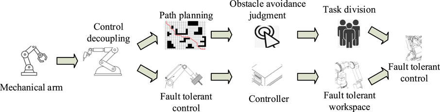
Figure 1. FTC process of an RA.

In Figure 1, the control decoupling of the RA is first carried out concurrent with the FTC. The FTC of the RA is divided into two main control directions. One is to carry out obstacle avoidance path planning for the RA, to judge the obstacle avoidance process of the RA through the algorithmic model, and to divide the obstacle avoidance task through the obstacle avoidance effect. The other part is to carry out coupling FTC for the RA by building a coupling sliding mode (SM) FT controller. Finally, the two different control modules are combined to realize FTC of the RA.

The A-star algorithm is used in the study to optimize the RA’s movement path and obstacle avoidance planning. The traditional A-star algorithm has defects such as slow planning. Therefore, to enhance the algorithm’s path search capability, a heuristic function optimizes the algorithm’s search path. Equation 1 is the heuristic function formula.

$f_F\left(x\right)=l_{1}a\left(x\right)+l_{2}b\left(x\right)+l_{3}c\left(x\right).(1)$

In Equation 1, $f_F\left(x\right)$ is the optimization heuristic function. $x$ is the parameter. $l_1$, $l_2$, and $l_3$ denote the weight coefficients. The range of $l_i$ belongs to 0–1 and satisfies $l_1+l_2+l_3=1$. $a\left(x\right)$, $b\left(x\right)$, and $c\left(x\right)$ denote the different maneuverable performance of the RA, such as operation cost and operation benefit. The heuristic function can optimize the motion performance (MP) of the RA and then guarantee the motion safety of the RA (Pham et al., 2023). The traditional A-star algorithm, when planning the RA motion process, will lead to poor path optimization due to the turning and movement of the RA and might even cause a secondary RA collision problem. Therefore, to optimize the RA motion path, this study uses Bessel curves for path optimization. Equation 2 is the curve expression.

$O\left(t\right)={\displaystyle \sum _{i=1}^n}{o}_i{C}_{i,n}\left(t\right).(2)$

In Equation 2, $O\left(t\right)$ is the Bessel curve. $t$ is the time variable. $C_{i,n}\left(t\right)$ denotes the $i$ th Bessel polynomial of the $n$ th Bessel curve. $o_i$ denotes the three-dimensional coordinates of the control points. The polynomial expression is shown in Equation 3.

$C_{i,n}\left(t\right)=\frac{n!}{i!\left(n-i\right)!}{t}^i{\left(1-t\right)}^{n-i}.(3)$

In Equation 3, the calculation of $C_{i,n}\left(t\right)$ is expressed as a combination of $i$ elements selected from $n$ different elements. The equation for the change in the curve with respect to time is shown in Equation 4 (Zhu et al., 2024; Nava and Pucci, 2023).

$j\left(t\right)=\frac{{\dot{o}}_x\left(t\right){\ddot{o}}_y\left(t\right)-{\dot{o}}_y\left(t\right){\ddot{o}}_x\left(t\right)}{{\left({\dot{o}}_x^2\left(t\right)+{\ddot{o}}_y^2\left(t\right)\right)}^{1.5}}.(4)$

In Equation 4, $\dot{o}\left(t\right)\ddot{o}\left(t\right)$ denotes the first-order partial derivative with respect to the time variable $t$. $\ddot{o}\left(t\right)$ the second order partial derivative with respect to the time variable $t$. Equation 1 optimizes path search through heuristic functions, with the goal of minimizing overall cost and maximizing motion performance. Equations 2–4 introduce Bezier curve smoothing paths, transforming the optimization problem into time parameterized trajectory optimization. The improved A-star algorithm (IASA) optimizes and maps the motion path of the RA into the new 3D space. Then, the optimization is performed by Bessel curves to improve the motion planning ability of the robot. At the same time, this study added a motion control model to improve the precision control of robot motion. Equation 5 is the formula for the motion control state.

$\left\{\begin{array}{l}{x}^{\prime }\left(t\right)=f\left(x\left(t\right),u\left(t\right),t\right),\\ y^{\prime }\left(t\right)=j\left(x\left(t\right),u\left(t\right),t\right).\end{array}\right.(5)$

In Equation 5, $x^{\prime }\left(t\right)$ denotes the derivative of the state vector at time $t$. $y^{\prime }\left(t\right)$ denotes the derivative of the output vector at time $t$. $u\left(t\right)$ denotes the control input vector. When the desired output state and operation state are already known, the learned control is obtained within a limited time range. Learning is carried out through iteration so that the current $u\left(t\right)$ is close to the control output of the next state, then the system output state at this time is close to the system output of the next state. Equation 6 is the tracking error expression (Nguyen et al., 2023; Zhu et al., 2023).

$a_k\left(t\right)=y_d\left(t\right)-y_k\left(t\right).(6)$

In Equation 6, $a_k\left(t\right)$ is the RA motion control error signal. $y_d\left(t\right)$ is the desired output value of the robot arm. $y_k\left(t\right)$ is the actual output value of the RA. The control flow of the RA after using the iterative algorithm is shown in Figure 2.

Figure 2

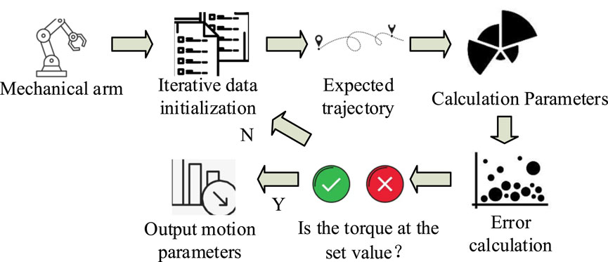
Figure 2. RA control process using an iterative algorithm.

In Figure 2, the RA is controlled by the iterative algorithm, which will first iterate the motion parameters of the RA. The desired trajectory of the RA is obtained after going through several iterations. Then, the kinematic intervention of the RA is used to calculate the motion parameters of the RA, such as the motion angle and angular velocity, and the moment of the RA is calculated. Then, the motion parameters of the actual RA are calculated by interfering with the moments. Finally, the motion error value of the RA is calculated based on the data parameters. The current moment magnitude of the RA is judged to be equal to the set value or not. If it is equal, the current RA motion parameters are output. If the values are not equal, the number of iterations must be increased to recalculate the RA moment until the current moment magnitude matches the set threshold.

2.2 Design of fault-tolerant robot arm sliding mold motion

FTC of the RA contains path planning and obstacle avoidance. The obstacle avoidance planning of the RA can improve its motion obstacle avoidance. Meanwhile, it is necessary to use a new controller to realize the motion FTC of the RA. As the motion gain of the RA must meet the large fault variation, the SM controller is able to estimate the attitude of the system. It also realizes the convergence of parameter error by adjusting the system parameters and has good application for nonlinear and uncertain data (Han et al., 2024). Therefore, the use of an adaptive SM controller is investigated to achieve FTC of an RA. The study adds the limit learning algorithm to the SM to improve the operation of the SM and reduce the risk of overfitting. Figure 3 shows the operation flow of the limit learning algorithm.

Figure 3

Figure 3. Running process of the extreme learning algorithm.

In Figure 3, the network will first initialize the input data during the network implementation. Then, the input data size of the hidden layer (HL) is obtained by the weight size and offset. After that, the output matrix of the HL is calculated according to the change of the input weight vector (WV). After completing the output of the HL, another output weight of the HL is set, and then the final output value is obtained by matrix calculation. An extreme learning network cannot adjust the weights and bias size again after completing the data initialization. However, a definite matrix size can be obtained by one-time data initialization, which improves the functional relationship of the uncertain problem. Equation 7 is the sample error data matrix expression.

$‖J\left(x,b,w\right)\dot{\rho }-Y‖=\underset{\rho }{\min }‖J\left(x,b,w\right)\rho -Y‖.(7)$

In Equation 7, $‖J\left(x,b,w\right)\dot{\rho }-Y‖$ denotes the error matrix. $J\left(x,b,w\right)$ denotes the function with input value $x$, bias $b$, and HL weights $w$. $\rho$ is the WV. $\dot{\rho }$ denotes the optimal solution of the WV. $Y$ denotes the target output matrix. At this point, the paradigm expression of the output matrix is shown in Equation 8 (Le and Yang, 2024; Li Y. et al., 2023).

$\dot{\rho }=J^{*}Y.(8)$

In Equation 8, $J^{*}$ denotes the generalized inverse matrix of the error matrix. The inverse matrix expression is obtained by matrix variation, as shown in Equation 9.

$J^{*}={\left(J^{T}J\right)}^{-1}{J}^T.(9)$

In Equation 9, $J^T$ denotes the inverse matrix. Equation 10 displays the ideal solution for the HL weights.

$J^{*}={\left(J^{T}J\right)}^{-1}{J}^{T}Y.(10)$

The weights and bias sizes in the current limit learning network are calculated by adjusting the matrix of the FT system of the RA to output the best function values. The FTC model of the RA defines the change of the motion trajectory error of the RA, as shown in Equation 11.

$a=z_1-z_d.(11)$

In Equation 11, $a$ denotes the motion trajectory error. $z_1$ denotes the actual motion trajectory of the RA. $z_d$ denotes the desired motion trajectory of the RA. The error kinematics of the SM can be described as shown in Equation 12.

$\left\{\begin{array}{l}\dot{a}={\stackrel{\sim }{z}}_2-{\stackrel{⌢}{z}}_d,\\ \stackrel{\dots }{a}=M^{-1}\left(z_1\right)\kappa +g\left(z_1,{\stackrel{\sim }{z}}_2\right)+f\left(z_1,z_2,\kappa \right)-{\stackrel{⌢}{z}}_d.\end{array}\right.(12)$

In Equation 12, $\dot{a}$ denotes the estimated value of the error. $z_2$ denotes the RA state variable. ${\stackrel{\sim }{z}}_2$ denotes the estimated value of the RA state variable. ${\stackrel{⌢}{z}}_d$ denotes the second order derivative of the desired trajectory. $\kappa$ denotes the moment of the mechanical arm. $g\left(z_1,{\stackrel{\sim }{z}}_2\right)$ denotes the gravity between the actual trajectory of the RA and the estimated value of the RA state variable. $f\left(z_1,z_2,\kappa \right)$ denotes the non-conservative force between the actual motion trajectory of the RA, the state variables, and the moment. $M^{-1}$ denotes the inverse matrix of the RA inertia matrix (IM), and $\stackrel{\dots }{a}$ denotes the second order derivative of the error. The use of third-order derivatives in the equation provides more accurate fault compensation and suppresses higher-order nonlinear effects. The conventional state equation does not explicitly include the output equation derivative, but in error dynamic analysis or specific control strategies, the output derivative may indirectly participate through state variables. The SM FT controller is generally categorized into three aspects: equivalence, fault identification, and function adaptation control. The controller is shown in Equation 13 (Zhu and Wang, 2024; Yang et al., 2023).

$\chi ={\chi }_e+{\chi }_f+{\chi }_a.(13)$

In Equation 13, $\chi$ denotes controller control torque. ${\chi }_e$ denotes controller equivalent torque control. ${\chi }_f$ denotes controller control fault identification compensation. ${\chi }_a$ denotes controller function control term. At this point, the equation of equivalent control changes as shown in Equation 14.

${\chi }_e=M\left(z_1\right)\left({\stackrel{⌢}{z}}_d-g\left(z_1,{\stackrel{\sim }{z}}_2\right)-{\eta }_1\dot{a}-\frac{p{\eta }_2}{l}{\left|a\right|}^{\frac{p-l}{l}}\dot{a}\right).(14)$

In Equation 14, $M$ is the IM of the RA. ${\eta }_1$ denotes the error variation related to the control gain. ${\eta }_2$ denotes the SM FT controller control gain. Both $p$ and $l$ denote exponential parameters. The fault identification compensation of the controller is shown in Equation 15 (Zhang et al., 2023; Long et al., 2023).

${\chi }_f=M\left(z_1\right)\ddot{\Delta }.(15)$

In Equation 15, $\ddot{\Delta }$ denotes the fault estimate. The final built SM FT controller is shown in Figure 4.

Figure 4

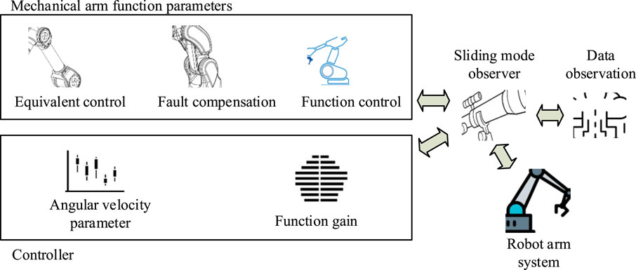
Figure 4. Sliding mode FT controller.

In Figure 4, the SM FT controller will build the SMC module through equivalent control, fault compensation, and function control during operation. The control module controls the joint angular velocity parameter and the function gain variation of the SM. Then, the controlled trajectory of the robot arm is observed by the SM observer. Meanwhile, the observer controls the SMC module through the non-singular SM surface. Moreover, the data parameters of the SMC module are input to the RA system to control the operation of the RA. The running mechanical table also transmits data to the SM observer in real time to complete the closed loop of data parameters. The core idea of SMC is to design a sliding surface and use a control law to force the system state to reach the surface within a finite time. Then, the system slides along the surface to the equilibrium point. The sliding surface formula is shown in Equation 16.

$S\left(t\right)=\dot{e}\left(t\right)+\lambda e\left(t\right).(16)$

In Equation 16, $S\left(t\right)$ denotes the sliding surface definition. $\dot{e}\left(t\right)$ denotes the error derivative. $e\left(t\right)$ denotes the error. $\lambda$ denotes a constant. The equivalent control term formula for the SM controller is shown in Equation 17.

$\tau ={\tau }_{eq}+{\tau }_{sw}+{\tau }_{fc}.(17)$

In Equation 17, ${\tau }_{eq}$ denotes the equivalent control torque. ${\tau }_{sw}$ denotes the switching control torque. ${\tau }_{fc}$ denotes the compensation control torque. The equivalent control formula is given by Equation 18.

${\tau }_{eq}=M\left(q\right)\left({\ddot{q}}_d+\lambda \dot{e}\right)+C\left(q,\dot{q}\right)\dot{q}+G\left(q\right).(18)$

In Equation 18, $M\left(q\right)$ represents the IM of the RA, $C\left(q,\dot{q}\right)$ represents the centripetal force matrix, and $G\left(q\right)$ represents the gravitational force matrix. The switching control torque formula is shown in Equation 19.

${\tau }_{sw}=-K·sign\left(s\right).(19)$

In Equation 19, $K$ represents the gain matrix, which determines the interference resistance capability. The FT compensation torque is shown in Equation 20.

${\tau }_{fc}=\stackrel{\sim }{F.}(20)$

In Equation 20, $\stackrel{\sim }{F}$ represents the fault estimate based on the observer. An SM observer is used to estimate the fault state of the RA in real time. First, the input data are initialized, and then it is mapped through a nonlinear activation function. Finally, the optimal weights are determined using the least squares method to minimize observation error. The fault recognition model process is shown in Equation 21 as an additive fault recognition formula.

${\tau }_{actual}={\tau }_{command}+F\left(t\right).(21)$

In Equation 21, ${\tau }_{actual}$ represents the actual execution torque. ${\tau }_{command}$ represents the command excitation. $F\left(t\right)$ represents the fault function. The identification of multiplicative faults is shown in Equation 22.

$y_{measured}=\left(1-\alpha \right)y_{true}+\beta .(22)$

In Equation 22, $y_{measured}$ represents the measured output value. $y_{true}$ represents the true output value. $\alpha$ represents the gain deviation. $\beta$ represents the offset. Equation 22 constructs the state estimation error and analyzes the magnitude of the error value. An error value that approaches 0 indicates the presence of a fault.

2.3 Design for the FTC of an RA system

A new FTC for an RA system can be built by path optimization and obstacle avoidance of the RA, improving the A-star algorithm to optimize the running route of the RA’s movement process. The SM FT controller is constructed for obstacle avoidance planning. Figure 5 shows the FTC process of the RA.

Figure 5

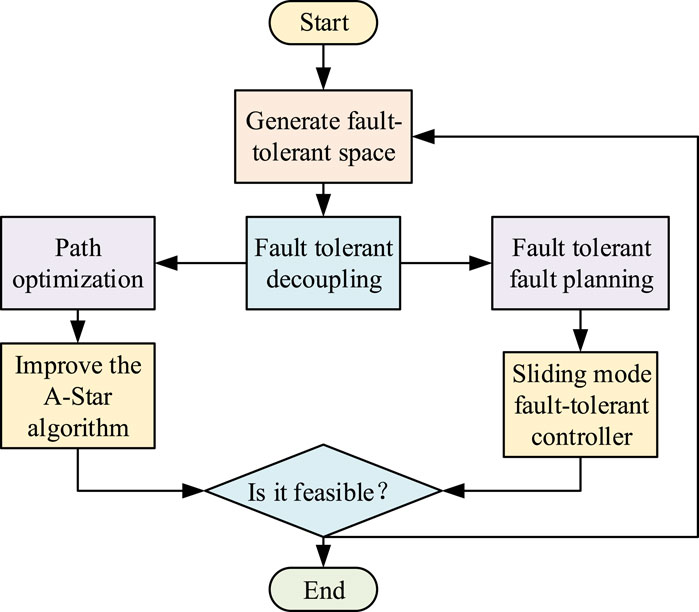
Figure 5. FTC process of an RA.

In Figure 5, the FT system generates an FTC space when the RA fails during motion. Then, two FTC paths are generated by decoupling the FT space through FT decoupling. The FT path optimization and generation are implemented using the IASA. FT fault planning is implemented by an SM FT controller. Finally, the FTC results in both directions are judged for feasibility. If the feasibility of the current task can be carried out, then the process ends. If the feasibility cannot be carried out, then the FTC is repeated until the feasibility of the current task can be carried out. To realize FTC of the robot arm, the research also builds a new experimental control system, as shown in Figure 6.

Figure 6

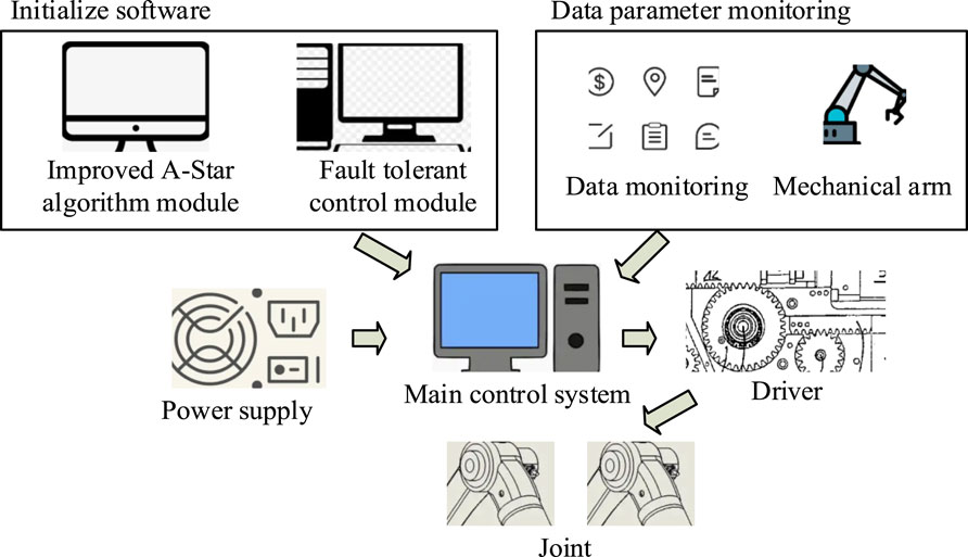
Figure 6. Experimental control system.

The total control system of the RA, as shown in Figure 6, includes two main parts. The first part is the controller initialization software, which contains the IASA module and the FTC module. The second part is the RA monitoring software, which is responsible for monitoring the faults and operating parameters of the RA. Both parts are operated through the control host. The control host also controls several major components of the robot arm, including the main control chip, the electromechanical driver, and the main control power supply. The electromechanical driver controls the joint changes of the robot arm through encoders and DC motors. Furthermore, during the entire FTC process, the data parameters of the robot arm can be presented on the host computer for better observation of the data parameter changes.

3 Effect analysis of FTC of the RA system

3.1 Analysis of the effect of RA path optimization

To test the actual operating effect of the RA using the FT system in the high-radiation environment of the nuclear industry, the study analyzes the optimization effect of the FT path of the RA. The study uses a six-degree-of-freedom RA for fault-tolerance testing, and OpenModelica simulation software is used for the study. Three different-sized obstacles are placed in the movement of the RA. The obstacle sizes are 0.20 m × 0.20 m × 0.20 m, 0.35 m × 0.3 m × 0.3 m, and 0.35 m × 0.40 m × 0.40 m, respectively. The programming language used for the study is Java. Comparative tests are conducted using the time-elastic band (TEB) algorithm, the rapidly exploring random tree (RRT) algorithm, and the simulated annealing (SA) algorithm. Table 1 shows the path optimization performance test results.

Table 1

Table 1. Performance comparison results of different algorithms for path optimization.

Table 1 shows the comparison of the different algorithms. The shortest running time of the IASA is only 1.24 s, compared with the TEB algorithm, which is an improvement of 1.92 s. IASA can reach 31 nodes, making it more able to optimize the RA. The path cost of the IASA is the lowest, only 0.48 m, which is 1.46 m lower than the RRT algorithm. This shows that the IASA has a better path planning effect, and it can make the RA complete the avoidance of obstacles under a shorter path. Finally, the MP of the IASA is 99%, which is 13% better than the RRT algorithm. It can be observed that the IASA has a very good path planning effect, which is due to the IASA adding limit learning. To test the test effect of different algorithms in the same environment, the study compares the test results of different algorithms in different paths, as shown in Figure 7. The path movement is selected as the indoor movement scene and the outdoor movement scene, respectively. The indoor movement adds obstacles such as chairs and tables, and the indoor scene has only a single obstacle. Scenario 1 is the indoor scene, and Scenario 2 is the outdoor scene.

Figure 7

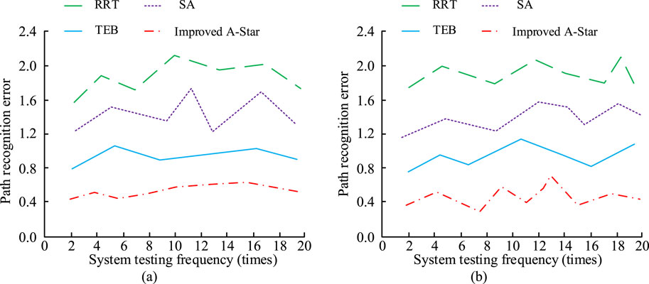
Figure 7. Comparison results of algorithm path errors in different scenarios. (a) Scenario 1, (b) Scenario 2.

In Figure 7a, in the indoor scene, there is only a single obstacle, improving the A-star algorithm with the smallest change in path error of only 0.4 m. Among the other algorithms, the RRT algorithm’s path deviation can reach a maximum of 2.2 m. It can be concluded that in the indoor scene, the actual planning effect of the IASA is much better, which may be because of the added limit learning. In Figure 7b, the path error of the IASA in the outdoor scene is also the smallest, with a maximum error of only 0.6 m, while the error value of the RRT algorithm is a maximum of 2.1 m. Compared with the RRT algorithm, the IASA’s error has been reduced by 1.5 m, which indicates that the IASA has a better operation and path planning effect in the outdoor scene. To test the actual path running effect of the algorithm model, the study compares the path length changes of different algorithms, as shown in Figure 8.

Figure 8

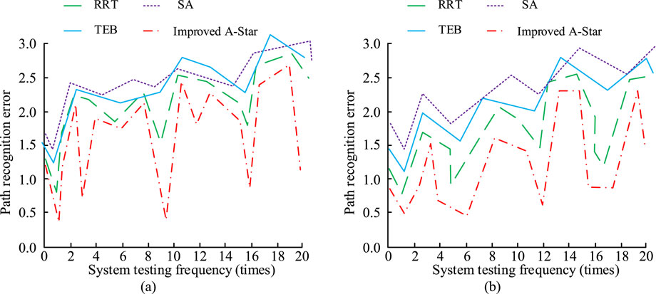
Figure 8. Comparison results of algorithm path length changes in different scenarios. (a) Scenario 1,(b) Scenario 2.

In Figure 8a, in Scenario 1, the motion path length change of the IASA is the smallest, and the maximum length change value is 2.3 m. The motion length change of the TEB is the largest, and the maximum length change is 3.0 m, which is 0.7 m more than that of the IASA. In the process of the RA motion, IASA has the smallest change in motion length and is more capable of motion planning, reducing the change in motion, and improving the overall operation effect. In Figure 8b, the motion length change of the IASA is also the smallest in different scenarios, and the highest motion length is only 2.0 m. In contrast, the motion length of the SA algorithm is the largest at this time, reaching a maximum of 2.8 m, which is 0.8 m longer than IASA. It can be observed that the change in the running path of the IASA in different scenarios has a lower value. This indicates that the IASA can effectively improve the motion trajectory fault tolerance of the RA.

3.2 Control analysis of the motion fault-tolerant module

The study compares and analyzes the change in motion of the RA under SMC. The study compares the change in motion control of the robot under different FTC methods. It analyzes the results of the change in the angle of different joint positions of the RA, which are tested in PID and model predictive control (MPC), respectively. Figure 9 shows the results of joint motion variation control.

Figure 9

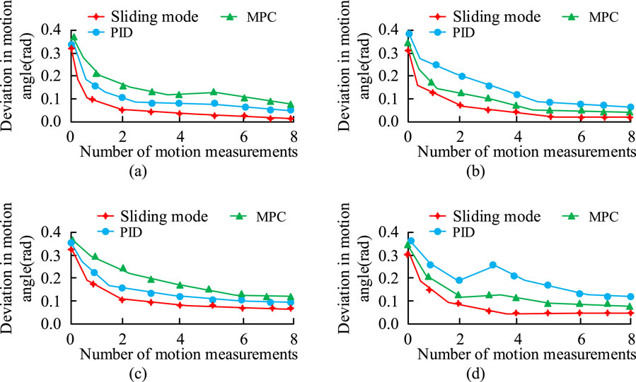
Figure 9. Comparison of joint control results using different methods. (a) Sports Joint 1, (b) Sports Joint 2, (c) Sports Joint 3, (d) Sports Joint 4.

Figures 9a–d show that the SMC method has better joint control than the other methods tested. Among them, the smallest joint error value is only 0.04 rad, which occurs at joint point 1. At the same time, the PID method has the worst control effect among the different control methods. Among them, the worst control effect is at joint point 4, when the maximum joint deviation is 0.25 rad. Moreover, the use of the control method at different joints is better than the other control methods, and the angular deviation value of the joints is smaller. This indicates that the use of SMC can improve the movement effect of the RA and improve the FTC ability of the RA. The results of testing the different direction deviations of the RA under different control methods are shown in Figure 10.

Figure 10

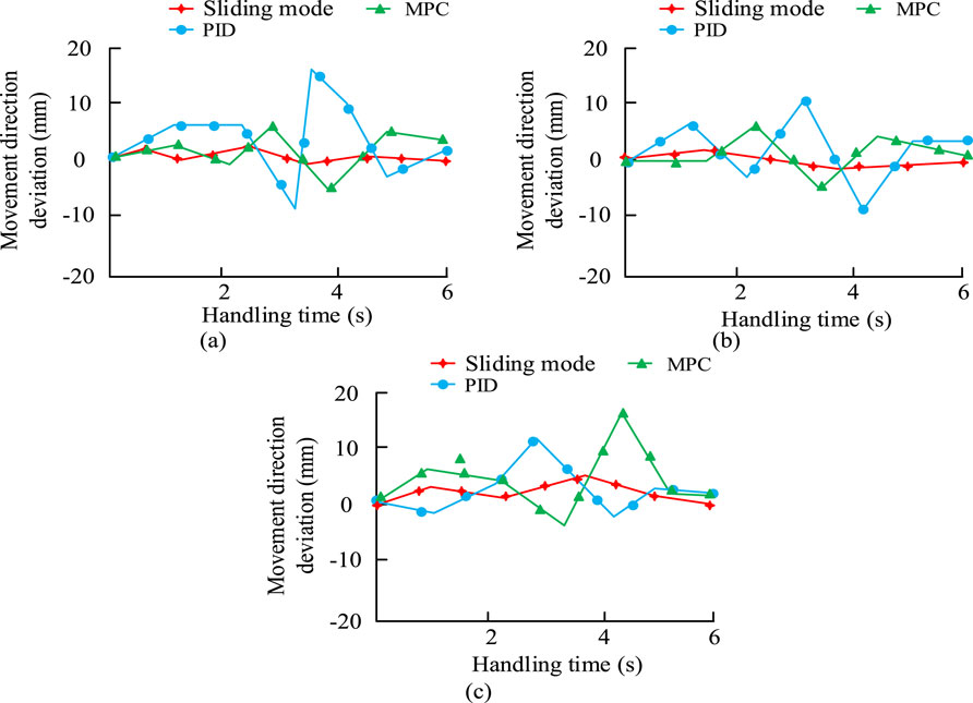
Figure 10. Comparison of motion deviations of RAs using different methods. (a) X-axis direction, (b) Y-axis direction, (c) Z-axis direction.

Figures 10a–c show that the SM controller used for the study has better control in different directions of RA movement. Among them, the maximum deviation in the X-axis is only 2 mm, in the Y-axis is only 1 mm, and in the Z-axis is only 5 mm. The PID control is the least effective. The maximum deviation in the X and Y axes can reach 15 mm and 10 mm, respectively. It can be concluded that the SMC has a better control effect in different directions, and its moving deviation is smaller, which may be because the SMC improves the torque control of the RA. The results of comparing the different control systems are shown in Table 2.

Table 2

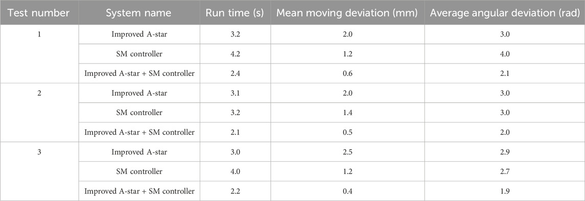
Table 2. Performance test results of different methods.

In Table 2, the control of the RA is relatively poor when only the IASA and the SMC are used. In this case, the system running time reaches a maximum of 4.2 s at a test count of 1, when only SMC is used. This indicates that the FTC time of the RA is longer when only SMC is used. After adding the IASA, the running time of the robot arm decreased by 1.8 s. Meanwhile, the angular deviation of the robot using only the IASA and the SMC is smaller than that of any of the other tests. It can be concluded that the combined use of the two control methods can significantly improve the FTC effect of the RA.

4 Conclusion

The study proposed an FTC for RAs method based on IASA to reduce the damage to an RA in a high-radiation environment. The study first accomplished the motion trajectory planning and obstacle avoidance of the RA by improving the A-star algorithm. Second, the SMC was used to improve the FTC of an RA. The research results indicated that the running time using IASA was reduced by 1.92 s compared with the TEB algorithm. At the same time, the path cost of the IASA decreased by 1.46 m compared with the TEB algorithm. The MP of the IASA could reach up to 99%. In different scenarios, the path deviation of the IASA compared with the RRT algorithm was 1.8 m lower. In outdoor scenarios, the path deviation of the IASA was 1.5 m lower. In the change of motion length, the IASA decreased by 0.8 m compared with the SA algorithm. The SMC of the RA had less angular deviation than that of the PID method, which was only 0.04 rad. The SMC had a better control effect in the variation of motion errors in different directions of axes, and the minimum deviations were only 2 mm, 1 mm, and 5 mm, respectively. The FTC effect of the system was significantly improved after using the IASA and the SMC. It can be concluded that the use of IASA and SMC can significantly improve the FTC effect of the RA. While the research has the potential to increase the efficacy of FTC of RAs, it is important to acknowledge the limitations of the study. For instance, the present study exclusively investigates robots operating in nuclear environments. There is a need to extend the research to other robots in diverse environments and categories. The present study exclusively explores the variation of the FTC error of robots. Other control parameters of robots will be analyzed in a subsequent study.

Data availability statement

The original contributions presented in the study are included in the article/supplementary material, further inquiries can be directed to the corresponding author.

Author contributions

NH: Conceptualization, Methodology, Writing – original draft. JC: Data curation, Formal Analysis, Writing – review and editing.

Funding

The author(s) declare that no financial support was received for the research and/or publication of this article.

Conflict of interest

The authors declare that the research was conducted in the absence of any commercial or financial relationships that could be construed as a potential conflict of interest.

Generative AI statement

The author(s) declare that no Generative AI was used in the creation of this manuscript.

Any alternative text (alt text) provided alongside figures in this article has been generated by Frontiers with the support of artificial intelligence and reasonable efforts have been made to ensure accuracy, including review by the authors wherever possible. If you identify any issues, please contact us.

Publisher’s note

All claims expressed in this article are solely those of the authors and do not necessarily represent those of their affiliated organizations, or those of the publisher, the editors and the reviewers. Any product that may be evaluated in this article, or claim that may be made by its manufacturer, is not guaranteed or endorsed by the publisher.

References

Al-Dujaili, A., Cocquempot, V., Najjar, M. E., Pereira, D., and Humaidi, A. (2023). Fault diagnosis and fault tolerant control for-linked two wheel drive Mobile robots. Inmob. Robot Motion Control Path Plan. 1 (6), 403–437. doi:10.1007/978-3-031-26564-8_13

CrossRef Full Text | Google Scholar

Han, A., Yang, Q., Chen, Y., and Li, J. (2024). Failure-distribution-dependent H fuzzy fault tolerant control for nonlinear multilateral teleoperation system with communication delays. Electronics 13 (17), 3454–3455. doi:10.3390/electronics13173454

CrossRef Full Text | Google Scholar

Hwang, C. L. (2023). Cooperation of robot manipulators with motion constraint by real-time RNN-based finite-time fault tolerant control. Neurocomputing 556 (10), 126694–126695. doi:10.1016/j.neucom.2023.126694

CrossRef Full Text | Google Scholar

Le, Q. D., and Yang, E. (2024). Adaptive fault tolerant tracking control for multi-joint robot manipulators via neural network-based synchronization. Sensors 24 (21), 6837–6838. doi:10.3390/s24216837

PubMed Abstract | CrossRef Full Text | Google Scholar

Li, M., Zhang, J., Li, S., and Wu, F. (2023a). Adaptive finite-time fault tolerant control for the full-state-constrained robotic manipulator with novel given performance. Eng. Appl. Artif. Intell. 125 (1), 106650–106651. doi:10.1016/j.engappai.2023.106650

CrossRef Full Text | Google Scholar

Li, Z., Wang, W., Zhang, C., Zheng, Q., and Liu, L. (2023b). Fault tolerant control based on fractional sliding mode: crawler plant protection robot. Comput. Electr. Eng. 105 (1), 108527–108528. doi:10.1016/j.compeleceng.2022.108527

CrossRef Full Text | Google Scholar

Li, Y., Dong, S., Li, K., and Tong, S. (2023c). Fuzzy adaptive fault tolerant time-varying formation control for nonholonomic multirobot systems with range constraints. IEEE Trans. Intelligent Veh. 8 (6), 3668–3679. doi:10.1109/tiv.2023.3264800

CrossRef Full Text | Google Scholar

Long, X. M., Chen, Y. J., and Zhou, J. (2023). Development of AR experiment on electric-thermal effect by open framework with simulation-based asset and user-defined input. Artif. Intell. Appl. 1 (1), 52–57. doi:10.47852/bonviewaia2202359

CrossRef Full Text | Google Scholar

Milecki, A., and Nowak, P. (2023). Review of fault tolerant control systems used in robotic manipulators. Appl. Sci. 13 (4), 2675–2676. doi:10.3390/app13042675

CrossRef Full Text | Google Scholar

Nava, G., and Pucci, D. (2023). Failure detection and fault tolerant control of a jet-powered flying humanoid robot. In2023 IEEE Int. Conf. Robotics Automation (ICRA) 29 (4), 12737–12743. doi:10.1109/icra48891.2023.10160615

CrossRef Full Text | Google Scholar

Nguyen, V. T., Bui, T. T., and Pham, H. Y. (2023). A finite-time adaptive fault tolerant control method for a robotic manipulator in task-space with dead zone, and actuator faults. Int. J. Control, Automation Syst. 21 (11), 3767–3776. doi:10.1007/s12555-022-1069-5

CrossRef Full Text | Google Scholar

Pham, D. H., Huynh, T. T., and Lin, C. M. (2023). Fault tolerant control for robotic systems using a wavelet type-2 fuzzy brain emotional learning controller and a topsis-based self-organizing algorithm. Int. J. Fuzzy Syst. 25 (5), 1727–1741. doi:10.1007/s40815-023-01516-y

CrossRef Full Text | Google Scholar

Shahna, M. H., and Mattila, J. (2023). Exponential auto-tuning fault tolerant control of N degrees-of-freedom manipulators subject to torque constraints. 27(10):15852–15853.

Google Scholar

Watanabe, Y., and Hyon, S. H. (2024). Fault detection and fault tolerant control for water hydraulic robots driven by air-hydraulic servo booster. In2024 IEEE/SICE Int. Symposium Syst. Integration (SII) 8 (1), 1399–1404. doi:10.1109/sii58957.2024.10417169

CrossRef Full Text | Google Scholar

Yang, P., Su, Y., and Zhang, L. (2023). Proximate fixed-time fault tolerant tracking control for robot manipulators with prescribed performance. Automatica 157 (10), 111262–111263. doi:10.1016/j.automatica.2023.111262

CrossRef Full Text | Google Scholar

Yeom, J., Li, G., and Loianno, G. (2023). Geometric fault tolerant control of quadrotors in case of rotor failures: an attitude based comparative study. In 2023 IEEE/RSJ Int. Conf. Intelligent Robots Syst. (IROS) 1 (10), 4974–4980. doi:10.1109/IROS55552.2023.10341669

CrossRef Full Text | Google Scholar

Zhang, C., Xu, X., and Zhang, X. (2023). Dual heuristic programming with just-in-time modeling for self-learning fault-tolerant control of mobile robots. Optim. Control Appl. Methods 44 (3), 1215–1234. doi:10.1002/oca.2791

CrossRef Full Text | Google Scholar

Zhang, J. X., Ding, J., and Chai, T. (2024). Fault tolerant prescribed performance control of wheeled mobile robots: a mixed-gain adaption approach. IEEE Trans. Automatic Control 13 (11), 5500–5507. doi:10.1109/tac.2024.3365726

CrossRef Full Text | Google Scholar

Zhu, W., and Wang, L. (2024). Adaptive finite-time fault tolerant control for Robot trajectory tracking systems under a novel smooth event-triggered mechanism. Proc. Institution Mech. Eng. Part I J. Syst. Control Eng. 238 (2), 288–303. doi:10.1177/09596518231188495

CrossRef Full Text | Google Scholar

Zhu, Y., Zhu, W., Liu, J., Wang, Q. G., and Yu, J. (2023). Command-filtered finite-time fuzzy adaptive fault tolerant control of output-constrainted robotic manipulators with unknown dead-zones. IEEE Trans. Circuits Syst. II Express Briefs 70 (8), 2939–2943. doi:10.1109/tcsii.2023.3249188

CrossRef Full Text | Google Scholar

Zhu, Y., Liu, Z., Jiang, B., and Zhu, Q. (2024). Adaptive fixed-time fuzzy fault tolerant control for robotic manipulator with unknown friction and composite actuator faults. J. Frankl. Inst. 15 (6), 107025–107026. doi:10.1016/j.jfranklin.2024.107025

CrossRef Full Text | Google Scholar