Numerical simulation and experimental study on hydraulic characteristics of L-shaped baffle fishway

The rapid expansion of hydraulic infrastructure has profoundly disrupted fish migration pathways in riverine ecosystems. To address this challenge, this study investigated the fishway at China’s Zhuzhou Hub, comparing conventional L-type and H-type baffle designs. A mathematical framework based on the k-ε turbulence model was employed to characterize the hydraulic behavior of these structures, with numerical solutions derived via the finite volume method. A comprehensive 1:6 scale physical model was then used to validate hydraulic performance, analyzing flow field structure in pool chambers, velocity distribution at vertical slots, and water surface profile variations under varying water levels. Results demonstrate that the L-type baffle configuration yields slot velocities of 0.28–0.87 m/s (mean: 0.50–0.77 m/s), meeting the critical swimming requirements of the “Four Major Chinese Carps” (black carp, grass carp, silver carp, and bighead carp) (response velocity: 0.2 m/s; critical velocity: 1.3 m/s). The main flow exhibited a smooth S-shaped curvature with lower flow distortion than the H-type baffle, while low-velocity zones (<0.3 m/s) occupied over 50% of the chamber area, ensuring both fish passage efficiency and resting opportunities. Experimental observations showed strong agreement with simulation data, confirming the accuracy of the mathematical framework and numerical methodology. These findings provide robust theoretical and practical guidance for optimizing fishway designs to enhance migratory success and ecological sustainability in regulated rivers.

1 Introduction

China’s rapid economic growth has intensified demands for hydropower energy and flood control infrastructure, driving the expansion of hydraulic engineering projects (Bai et al., 2017; Liu et al., 2019; Yu and Chang, 2025). However, these developments often obstruct fish migration routes, necessitating the integration of fish passage facilities to mitigate ecological impacts. Fish passage is a specially designed channel for fish to help them move freely in rivers, lakes, and other water bodies, overcoming obstacles such as dams and weirs, thereby enabling them to complete their life history activities, including migration, foraging, and reproduction (Romao et al., 2018; Silva et al., 2018). Existing solutions include fish lifts, transport systems, gates, and fishways. While lifts and transport systems are suitable for medium-to high-head dams, their discontinuous operation, high costs, and logistical complexity limit their efficacy. In contrast, fishways—particularly pool-weir designs—are widely adopted for low-head applications due to their short construction span, rapid flow stabilization, and adaptability to fish behavior (Santos et al., 2014; Bomba et al., 2017).

Despite their prevalence, pool-weir fishways face challenges such as turbulent eddies that disrupt functionality (Francisco Fuentes-Perez et al., 2016; Romao et al., 2018). Extensive experimental and numerical studies have explored hydraulic performance optimization. Yuan et al. (2024) and Quaranta et al. (2019) demonstrated that pool flow patterns transition from two-dimensional (slope <5%) to three-dimensional (slope ≥10%) characteristics, with negligible vertical velocity components. Puertas et al. (2004) identified linear relationships between dimensionless discharge and flow depth in weir-type fishways, advocating for straight rectangular notches over zigzag or trapezoidal designs to enhance upstream migration. Kim (2001) corroborated these findings, emphasizing the importance of weir geometry.

Numerical studies have further advanced design insights. Bermudez et al. (2010) highlighted pool length as a critical parameter influencing flow dynamics in vertical slot fishways (VSFs). Dong et al. (2024) analyzed island-type fishways, revealing that valvular configurations with smaller arc angles expand high-velocity zones while reducing low-speed regions. Ahmadi et al. (2021) demonstrated that baffle angles and cylinder diameters in VSFs inversely affect flow velocity and turbulent kinetic energy. Abdolahipour (2024) conducted a comprehensive analysis of numerical simulation and experimental approaches for flow separation control, systematically evaluating the influence of key parameters such as excitation frequency (F+) and momentum coefficient (Cμ) on control effectiveness, while highlighting their advantages in reducing energy dissipation. Meanwhile, Sheikholeslam Noori et al. (2019) employed a multiple-relaxation-time color-gradient lattice Boltzmann model (MRT-CG LBM) with geometric wetting boundary conditions to handle contact angles, achieving stable simulations of two-phase flow problems with high density ratios (approximately 1,000:1). Qi et al. (2024) confirmed the three-dimensional flow characteristics and planar two-dimensional dominance in trapezoidal and vertical slot fishways, respectively.

Current fishway design must account for species-specific requirements, geographic variability, and economic constraints. To address these challenges, this study focuses on L-type and H-type baffle fishways—a novel configuration developed for low-head hydraulic projects with spatial limitations. Through an integrated approach combining mathematical modeling, numerical simulation (k-ε turbulence model), and experimental validation, we systematically analyzed key hydraulic characteristics including velocity distribution, turbulent intensity, and recirculation zones to optimize fish passage efficiency. This work establishes a design framework for enhancing fishway reliability, cost-effectiveness, and ecological compatibility, while providing actionable insights for sustainable river management.

2 Engineering overview

The baffle-type fishway employs staged energy dissipation to optimize flow patterns, making it particularly suitable for large water-level differentials while providing resting areas for fish. In this project, a vertical-slot baffle configuration was selected due to its strong adaptability, stable flow velocity characteristics, and construction convenience. The vertical-slot design enables precise control of both flow regime and velocity distribution, ensuring compliance with design specifications. This configuration demonstrates superior hydraulic regulation capability compared to conventional slot-type fishways and can accommodate fish species with varying depth preferences. A schematic diagram of the structure is presented in Figure 1, including outlet trash rack, fishway pool room, fish water flow at high water level, fishway inlet fish water flow, rest pool, and fishway inlet.

Figure 1

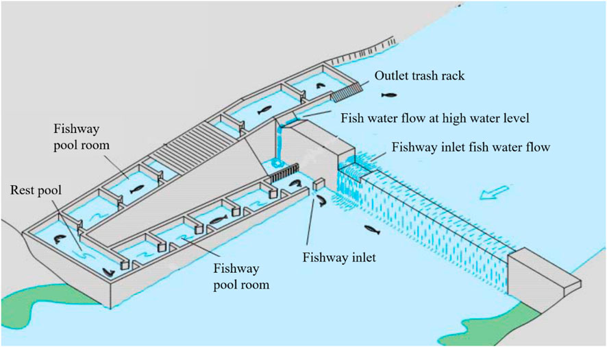
Figure 1. Fishway schematic diagram.

The engineering design adheres to ICOLD principles and China’s SL609-2013 guidelines, prioritizing: 1 velocity alignment with fish swimming capacity (0.2–1.3 m/s), 2 turbulence minimization through baffles, and 3 oxygenation via open-channel structures. Parameters were established for the Zhuzhou Hub on the mainstream Xiangjiang River in Hunan Province, China, where the fishway is located on the left bank slope of the Sanmen flood diversion channel. The 1,144 m-long fishway features a 1:107 bed slope, designed for the “Four Major Chinese Carps” (black carp, grass carp, silver carp, and bighead carp) with body lengths of 40–100 cm, widths <0.3 m, response threshold velocity of 0.2 m/s, and critical swimming speeds of 1.0–1.3 m/s. The vertical-slot design maintains 0.2–1.3 m/s velocities to accommodate migratory behavior, supplemented by a pulsed DC fish guidance system (0.5 V/cm field strength) that exploits electrotaxis to attract target species while excluding non-target organisms.

The fishway employs a transverse-baffle vertical-slot configuration, with 0.6 m-wide slots sized for target species and 3 m × 4 m chambers balancing cost-efficiency with passage performance. Channel width (B) scales with fish size and migration volume–wider designs reduce velocities for resting but increase costs. The adopted 3 m rectangular section optimizes economic and biological requirements. Chamber length affects energy dissipation; while longer chambers (≥4.0 m) lower velocities, they increase construction costs. The 4.0 m design reflects international best practices for cost-performance balance. Water depth ranges 1.0–3.22 m (maximum pool depth 3.30 m) to accommodate surface- and bottom-dwelling species while preventing overflow. This integrated system combines transverse baffles, vertical guide walls, and horizontal deflectors to modulate flow dynamics and facilitate fish passage, with “H”-type and “L”-type baffle configurations illustrated in Figure 2. The design simultaneously ensures fish transit/resting needs, economic viability, and engineering feasibility.

Figure 2

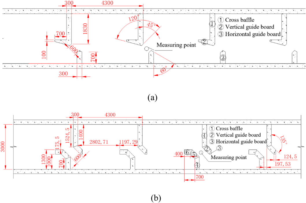
Figure 2. Structure of baffle fishway. (a) L-shaped baffle fishway (b) H-shaped baffle fishway.

Both the “H”-type and “L”-type baffle configurations represent recommended solutions in existing engineering projects, though their respective flow regimes may exhibit notable differences. The Zhuzhou and Dayandu fishways feature relatively mild bottom slopes, with preliminary estimates suggesting both configurations should satisfy the design velocity requirements. To enable quantitative comparison between these alternatives, this study employs a three-dimensional hydrodynamic model to conduct a comparative analysis of the hydraulic conditions generated by these two prevalent baffle types in Chinese fishway applications. Notably, the steeper bottom slope of the Zhuzhou fishway (1:107) was adopted for this study to ensure robust validation under more challenging hydraulic conditions. Consistent with this approach, the rest pool slope was also set to 1:107 to maintain hydraulic continuity and ecological compatibility.

3 Numerical solution and results analysis

3.1 Hydraulic model of the baffle fishway

To evaluate potential hydrodynamic differences between the two baffle types, 3D turbulent flow numerical models were developed. The governing equations adopted the Reynolds-averaged Navier-Stokes (RANS) formulation. For open-channel flow modeling, turbulence closure options typically include: the standard k-ε model (suitable for high-Reynolds-number flows with simple shear, such as straight channels, offering computational efficiency but limited accuracy); RNG/Realizable k-ε variants (recommended for complex flows involving curvature or rotation - with RNG emphasizing swirling flows and Realizable excelling in separated flows); and the SST k-ω model (preferred for high-accuracy requirements like separated flows or strong adverse pressure gradients, though demanding superior mesh quality and computational resources). Given the relatively simple flow characteristics and constrained computational resources, the standard k-ε model was selected as the turbulence closure scheme for this numerical simulation.

Assuming the river water behaves as an incompressible fluid and applying a two-equation turbulence model, the governing equations for the three-dimensional flow field were formulated, as shown in Equations 1–7:

Continuity equation of flow in the fishway:

$\frac{\mathit{\partial }{u}_i}{\mathit{\partial }{x}_i}=0(1)$

Momentum equation of flow in the fishway:

$\frac{\mathit{\partial }}{\mathit{\partial }\mathit{t}}\left(\mathit{\rho }{\mathit{u}}_{\mathit{i}}\right)+\frac{\mathit{\partial }}{\mathit{\partial }{\mathit{x}}_{\mathit{j}}}\left(\mathit{\rho }{\mathit{u}}_{\mathit{i}}{\mathit{u}}_{\mathit{i}}\right)=-\frac{\mathit{\partial }\mathit{p}}{\mathit{\partial }{\mathit{x}}_{\mathit{i}}}+\frac{\mathit{\partial }{\mathit{\tau }}_{\text{ij}}}{\mathit{\partial }{\mathit{x}}_{\mathit{j}}}+\mathit{\rho }{\mathit{g}}_{\mathit{i}}(2)$

equation $k$:

$\frac{Dk}{Dt}=\frac{\mathit{\partial }}{\mathit{\partial }{x}_i}\left[\left(\nu +\frac{{\nu }_t}{{\sigma }_k}\right)\frac{\mathit{\partial }k}{\mathit{\partial }{x}_i}\right]+G_k-\epsilon (3)$

equation $\epsilon$:

$\frac{D\epsilon }{Dt}=\frac{\mathit{\partial }}{\mathit{\partial }{x}_i}\left[\left(\nu +\frac{{\nu }_t}{{\sigma }_{\epsilon }}\right)\frac{\mathit{\partial }\epsilon }{\mathit{\partial }{x}_i}\right]+C_{1\epsilon }\frac{\epsilon }{k}{G}_k-C_{2\epsilon }\frac{{\epsilon }^2}{k}(4)$

which $t$ is time; $u_i$; $x_i$ is Velocity Component and Coordinate Component; ${\tau }_{ij}$ is stress tensor, definite is shown in Equation 5; $\nu$ is Kinematic viscosity coefficient; p is modified pressure; $\rho g_i$ is Gravitational force; ${\mu }_t=\mathit{\rho }{\mathit{\nu }}_{\mathit{t}}=\mathit{\rho }{\mathit{c}}_{\mathit{u}}{\mathit{k}}^2/\mathit{\epsilon }$ is turbulence viscosity coefficient; ${\delta }_{ij}$ is the Kronecker delta symbol; Experiential constant in equation $c_u=0.09$, ${\sigma }_k=1.0$, ${\sigma }_{\epsilon }=1.33$,

$C_{1\epsilon }=1.44$, $C_{2\epsilon }=1.42$; $G_k$ is the average velocity and gradient rising by turbulent kinetic energy.

${\tau }_{ij}={\mu }_t\left(\frac{\mathit{\partial }{u}_i}{\mathit{\partial }{x}_j}+\frac{\mathit{\partial }{u}_j}{\mathit{\partial }{x}_i}\right)-\frac{2}{3}{\delta }_{ij}\left(\rho k+{\mu }_t\frac{\mathit{\partial }{u}_i}{\mathit{\partial }{x}_j}\right)(5)$

$G_k={\nu }_t\left[\frac{\mathit{\partial }{u}_i}{\mathit{\partial }{x}_j}\left(\frac{\mathit{\partial }{u}_i}{\mathit{\partial }{x}_j}+\frac{\mathit{\partial }{u}_j}{\mathit{\partial }{x}_i}\right)\right](6)$

In computational fluid dynamics, the Volume of Fluid (VOF) method is commonly employed to model the free surface. This approach centers around a volume fraction function F, defined throughout the computational space. Numerically, F serves as a clear indicator of fluid distribution. Specifically, when F = 1, it corresponds to regions filled completely with pure water. Conversely, F = 0 designates non is water regions, such as the air above the liquid or the container’s solid boundaries. Intermediate values, where 0 < F < 1, precisely mark the free surface interface. This interface is where the water transitions to other substances, like air, with distinct physical properties.

The volume fraction function F is not static. Instead, it evolves continuously with both spatial coordinates (x, y, z) and time t, written as F = F (x, y, z, t). Conceptually, F can be thought of as a massless, neutrally buoyant tracer. As fluid particles move under the influence of pressure gradients, viscous forces, or gravity, this tracer adheres to them. This enables accurate tracking of the free surface’s movement in both space and time.

The transport equation is

$DF/Dt=0(7)$

3.2 Numerical solution method

Using Common Expression (1)-(4) can get Equation 8:

$\frac{\mathit{\partial }\varphi }{\mathit{\partial }t}+\nabla ·\left(u_j\varphi \right)=\nabla ·\left({\mathit{\Gamma }}_{\varphi }grad\varphi \right)+S_{\varphi }(8)$

which t and u_j is the time vector and velocity vector; φ is Common variable, such as velocity, turbulent energy; Г_Ф is Diffusivity coefficient of variable φ; S_φ is equation of source item.

The numerical solution process begins by applying triple integration to Equation 6. Using Gauss’ divergence theorem, the volume integral over an arbitrary control volume CV (bounded by surface A) is transformed into a surface integral. This transformation yields the fundamental equation of the finite volume method (FVM), as shown in Equation 9:

$\frac{\mathit{\partial }}{\mathit{\partial }t}{\int }_V\rho \varphi dV=-{\int }_{A}F\left(\varphi \right)·ndA+{\int }_V{S}_{\varphi }dV(9)$

which $F\left(\varphi \right)·n$ is the normal numerical flux.

Through volume averaging of the control element, the governing equation is discretized into its final form using the finite volume method (FVM) as shown in Equation 10:

$\frac{\Delta \left(\rho \varphi \right)}{\Delta t}=-\frac{1}{\Delta V}{\displaystyle \sum _{j=1}^m}{F}_j^n\left(\varphi \right)A_j+{\overline{S}}_{\varphi }(10)$

which $\Delta V$ is element volume; m is the total number of face; A_j is area of face j; ${\overline{S}}_{\varphi }$ is element average value of source item, normal flux of face j; $F_j=F_j\left(\varphi \right)·n$, including convective flux and diffusive flux.

For the definition of boundary conditions, the upstream inlet and downstream outlet boundaries are specified using the free surface water level as the respective boundary values. At wall surfaces, the Launder & Spalding wall function is applied to model near-wall turbulence. The turbulent kinetic energy k and dissipation rate ε at the inlet and outlet are calculated using the Equation 11 empirical formulas:

$K=0.00375u^2;\epsilon =K^{3/2}/0.4L(11)$

which L is length of turbulent flow pattern.

3.3 Results analysis

The 3D model of the L-shaped and H-shaped baffle fishway, depicted in Figure 3, spans a total length of 60.2 m and consists of 13 pool chambers and one resting pool. To enhance the accuracy of the numerical solution, the computational domain was discretized using hexahedral elements, as illustrated in Figure 4. The mesh comprises 461,100 nodes and 415,800 hexahedral cells, ensuring high resolution and efficient computation. The main flow streamline plot of the fishway are presented in Figure 5. As illustrated, the main flow exhibits a well-defined “S”-shaped curvature with a width approximating the vertical slot width (0.6 m). Compared to H-type baffle configurations, the L-shaped design demonstrates reduced curvature intensity, resulting in smoother flow trajectories that facilitate unimpeded fish passage without requiring abrupt directional changes.

Figure 3

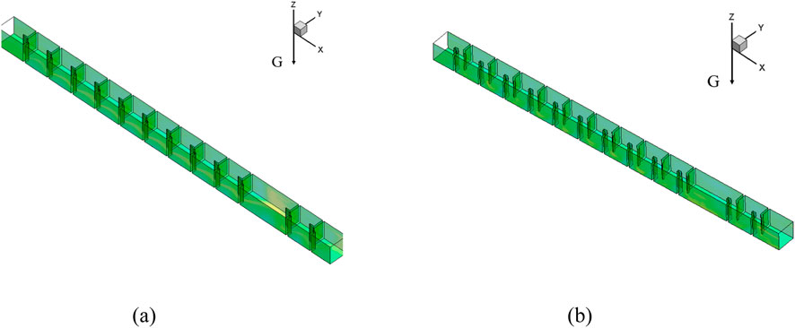
Figure 3. 3D geometry model of baffle fishway. (a) L-shaped baffle fishway (b) H-shaped baffle fishway.

Figure 4

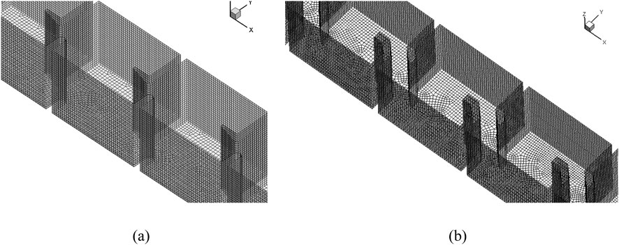
Figure 4. Mesh of baffle fishway. (a) L-shaped baffle fishway (b) H-shaped baffle fishway.

Figure 5

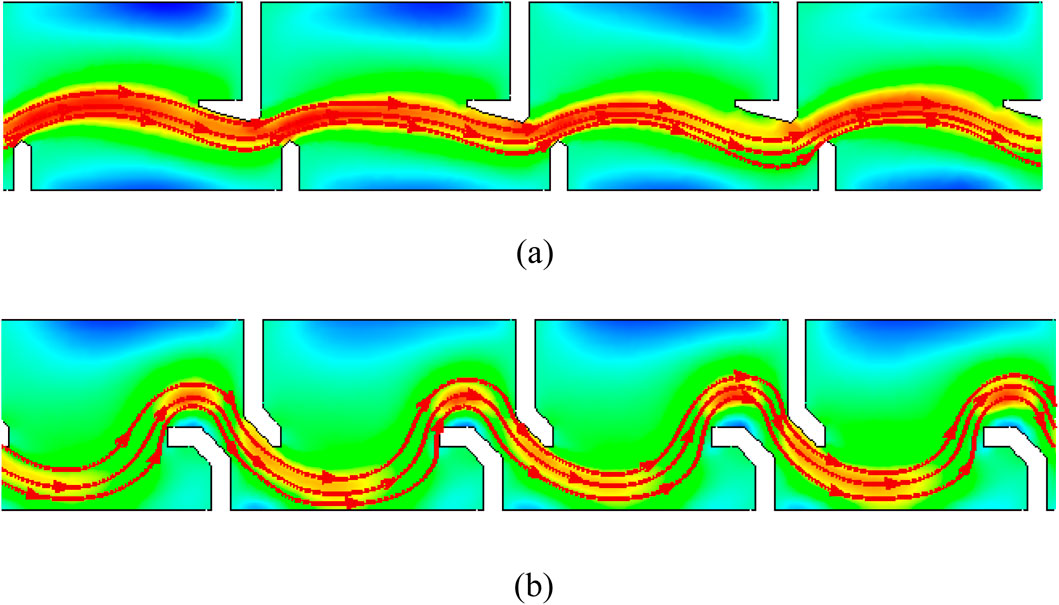
Figure 5. Mainstream streamlined diagram of the baffle fishway. (a) L-shaped baffle fishway (b) H-shaped baffle fishway.

Detailed examination of isopleth contours and velocity vector fields in Figures 6–9 demonstrates minimal velocity variation across depth layers (surface, mid-column, and bottom) due to the smooth cement boundary conditions. The maximum velocity of 0.8 m/s occurs at the vertical seam’s trailing edge, while extensive low-velocity zones (<0.2 m/s) flanking the mainstream provide refuge areas covering 42% of chamber volume.

Figure 6

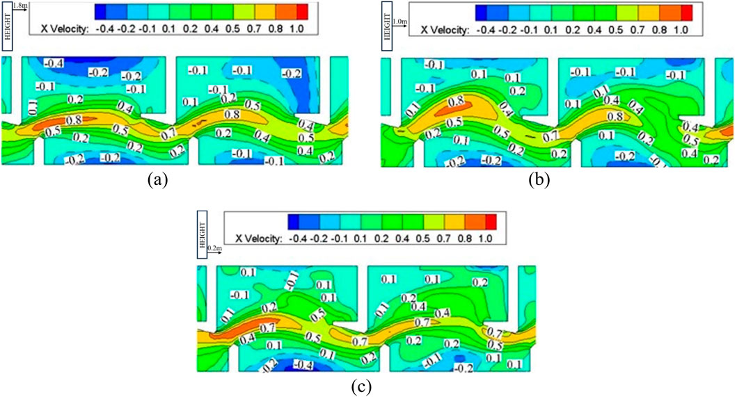
Figure 6. Flow velocity isopleth cloud atlas of pool room of the L-shaped baffle fishway. (a) Flow velocity isopleth cloud atlas at 1.8 m from the bottom (b) Flow velocity isopleth cloud atlas at 1.0 m from the bottom (c) Flow velocity isopleth cloud atlas at 0.2 m from the bottom.

Figure 7

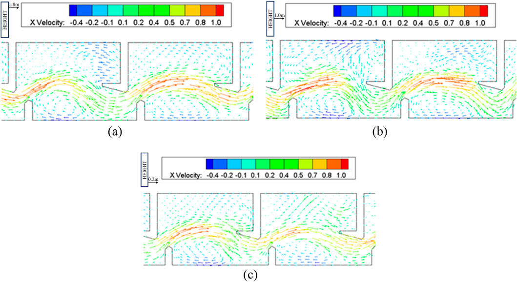
Figure 7. Vector graphics of flow velocity of pool room of the L-shaped baffle fishway. (a) Vector graphics of flow velocity at 1.8 m from the bottom (b) Vector graphics of flow velocity at 1.0 m from the bottom (c) Vector graphics of flow velocity at 0.2 m from the bottom.

Figure 8

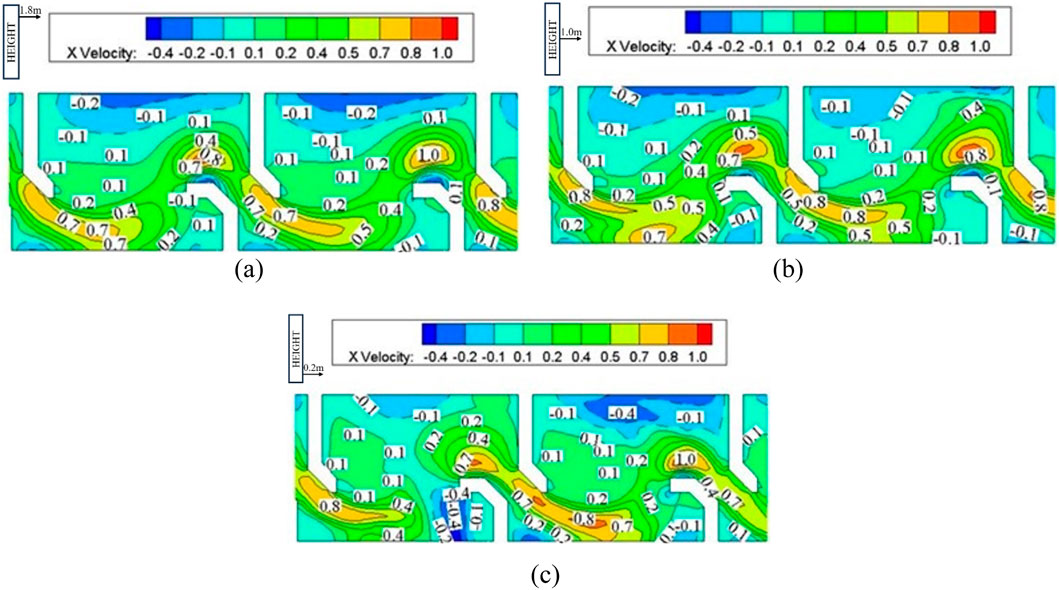
Figure 8. Flow velocity isopleth cloud atlas of pool room of the H-shaped baffle fishway. (a) Flow velocity isopleth cloud atlas at 1.8 m from the bottom (b) Flow velocity isopleth cloud atlas at 1.0 m from the bottom (c) Flow velocity isopleth cloud atlas at 0.2 m from the bottom.

Figure 9

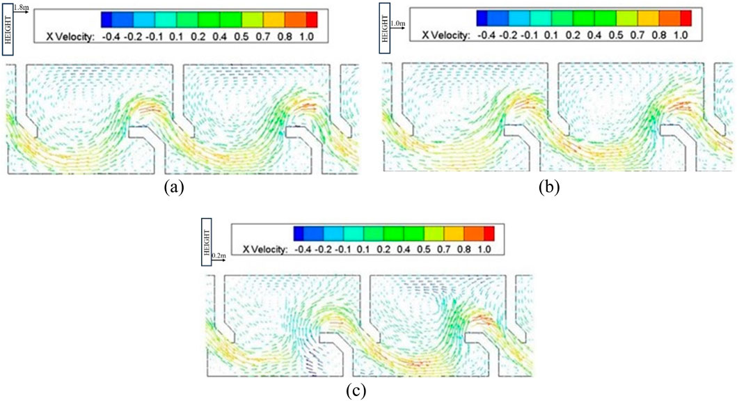
Figure 9. Vector graphics of flow velocity of pool room of the H-shaped baffle fishway. (a) Vector graphics of flow velocity at 1.8 m from the bottom (b) Vector graphics of flow velocity at 1.0 m from the bottom (c) Vector graphics of flow velocity at 0.2 m from the bottom.

To comprehensively assess the flow velocity distribution within the L-shaped baffle fishway, measurement sections were positioned within the pool chamber, as detailed in Figure 10. Each section incorporated 10 measurement points distributed uniformly across the surface, mid-layer, and bottom layer, yielding a total of 150 discrete measurement locations. Numerical simulations provided velocity data at these points, with results systematically compiled in Tables 1–3.

Figure 10

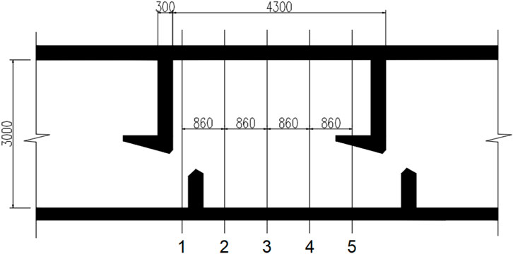
Figure 10. Flow measuring sections setup in the pool room.

Table 1

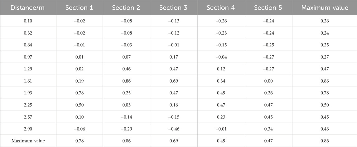
Table 1. The surface layer water flow velocity of L-shaped baffle (1.8 m from the bottom) (m/s).

Table 2

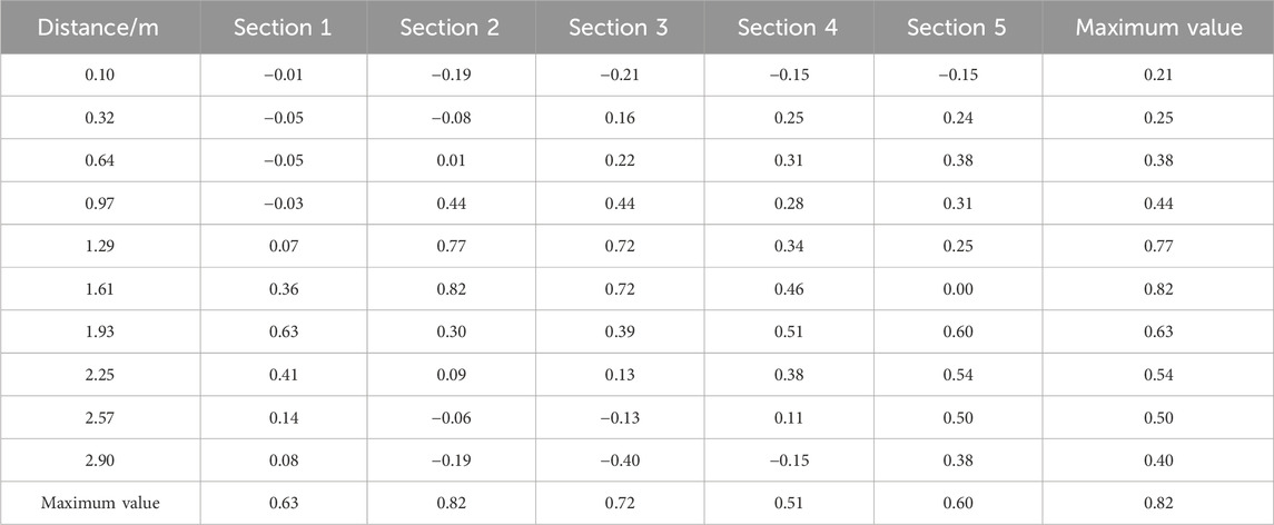
Table 2. The middle layer water flow velocity of L-shaped baffle (1.0 m from the bottom) (m/s).

Table 3

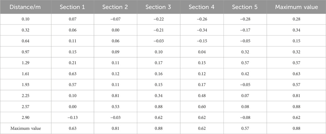
Table 3. The bottom layer water flow velocity of L-shaped baffle (0.2 m from the bottom) (m/s).

Analysis of the Tables 1–3 reveals a peak flow velocity of 0.88 m/s within the mainstream region of the pool chamber. Notably, only three measurement points (2.7% of the total) exceeded 0.8 m/s, confirming minimal high-velocity zones. Furthermore, a substantial portion of the chamber exhibited low-velocity conditions, with flow velocities consistently around 0.2 m/s. This low-flow zone serves as a critical refuge area, facilitating energy conservation for migrating fish. Collectively, the velocity characteristics of the L-shaped baffle fishway align with design specifications, maintaining velocities between 0.8 m/s and 1.0 m/s to ensure optimal fish passage conditions.

Numerical simulations further validated the hydraulic performance of the rest pool, as illustrated in Figures 11, 12. Velocity isopleths in Figure 11b demonstrate that most regions within the rest pool sustain velocities below 0.6 m/s, while Figure 11c confirms that over 50% of the area maintains velocities under 0.3 m/s, establishing an extensive low-velocity resting habitat. Velocity vector analysis in Figure 12 identifies two recirculation zones: a minor zone downstream of the left baffle and a larger zone adjacent to the mainstream. Despite their presence, velocity magnitudes within these recirculation zones remain below 0.2 m/s, as corroborated by the isopleth contours in Figure 8. Given their subdued flow intensity, these zones pose no significant impediment to fish movement and instead contribute to favorable resting conditions.

Figure 11

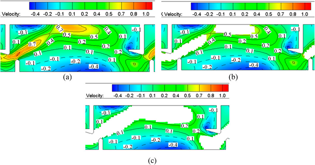
Figure 11. Flow velocity isopleth diagram of the rest pool. (a) No cover (b) Cover the flow velocity over 0.6 m/s (c) Cover the flow velocity over 0.3 m/s.

Figure 12

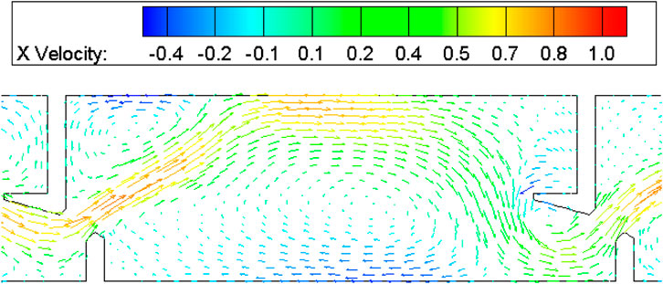
Figure 12. Flow velocity vector graphics of the rest pool.

Comparative evaluation of the H-type and L-type baffle configurations confirms that both satisfy fundamental hydraulic design criteria, exhibiting comparable bulk flow velocities. However, the H-type baffle induces pronounced flow distortion at the vertical slot entrance, whereas the L-type configuration promotes smoother flow trajectories, enhancing upstream fish passage efficiency. Based on these hydrodynamic advantages, the L-type baffle is recommended as the optimal design solution. Subsequent research phases will involve physical model testing to validate the hydraulic performance of the L-type baffle fishway configuration.

4 Experiment platform design and results analysis

4.1 Experiment platform design

To further validate the accuracy and reliability of the numerical simulation results for the L-shaped baffle fishway, a physical simulation experiment platform was constructed to test the flow conditions within the fishway. The vertical seam width of the L-shaped baffle fishway pool is relatively narrow, measuring only 60 cm. To accurately replicate the hydraulic conditions of both the pool chamber and the vertical seam, a geometric scaling ratio of L_r = 6 was selected for the construction of the physical model. The hydrodynamic model of the fishway was designed in accordance with the gravity similarity criterion, ensuring that the scaled model faithfully represents the flow dynamics of the prototype. Based on this approach, the following parameters were derived:

Velocity measuring scale, as shown in Equation 12:

$L_v={L_r}^{1/2}=2.45(12)$

Flow quantity measuring scale, as shown in Equation 13:

$L_Q={L_r}^{5/2}=88.2(13)$

The physical model was constructed using plastic boards and consists of 10 fish pool chambers and one resting pool, with a total of 12 baffles numbered sequentially from the bottom upward (1–12). The baffles are arranged with vertical seams on the same side, spaced 71.6 cm apart (measured as the center-to-center distance between adjacent vertical seam baffles). The model’s bottom slope is set at 1:107, and its layout is illustrated in Figure 13.

Figure 13

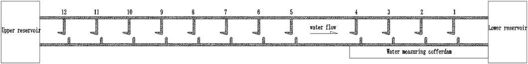
Figure 13. The local model layout (12 baffles numbered from the bottom up by 1–12).

The measurement point arrangement is shown in Figure 14. The vertical seam section is equipped with five measurement points, while each pool chamber contains three measurement sections (Sections 1–3). Each measurement section includes five measurement points distributed across five layers along the water depth. The experimental platform for the physical simulation is depicted in Figure 15.

Figure 14

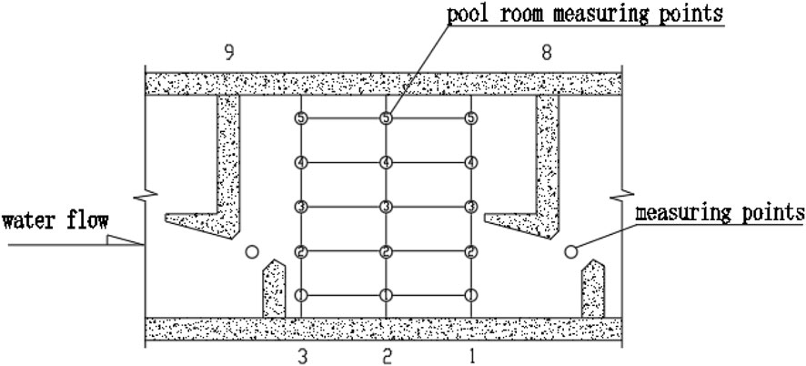
Figure 14. The layout of the model measurement point.

Figure 15

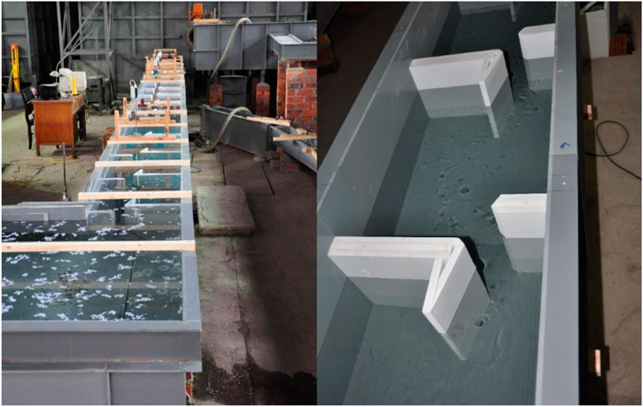
Figure 15. L-shaped baffle fishway of the physical simulation of the experiment platform.

To ensure the full development of the water flow in the test section, the upstream water level was controlled using a flat flume in the reservoir, while the downstream water level was regulated by an overflow plate. In the experimental platform, the water depth upstream and downstream of the model was maintained at 33.3 cm, corresponding to 2.0 m in the numerical model.

A wireless propeller current meter was employed to measure the flow velocity through the fish passage holes in the baffle plates. The flow field within the pool chamber was measured using a three-dimensional Acoustic Doppler Velocimeter (ADV). Additionally, the flow rate of the fishway was determined using a triangular weir, and the slope of the fishway chamber was monitored using a manometer. Because the test process is lossless, the test is repeated three times, and the average value of the three results is taken to improve the test accuracy and reduce the test error.

4.2 Experiment result analysis

Figure 16 presents the hydraulic characteristics observed within the pool chamber of the L-shaped baffle fishway. Comparative assessment with Figure 5 demonstrates that the L-type configuration preserves distinct main flow trajectories while minimizing flow distortion. The primary flow exhibits a smooth S-shaped profile through the chamber, accompanied by localized surface recirculation zones that maintain stable hydraulic conditions. The optimized jet angle (relative to the transverse baffle) prevents flow contraction at the orifice while promoting effective flow diffusion. Physical modeling results in Figure 16 further confirm the development of stable recirculation zones along both sides of the surface flow, with excellent agreement between experimental observations and numerical predictions.

Figure 16

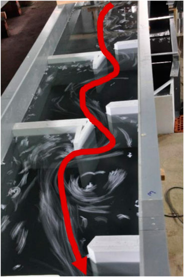
Figure 16. Flow state of the pool room in the L-shaped baffle fishway.

Quantitative evaluation of chamber velocities, measured at 18 cm above the pool bottom (Table 4), reveals that 96% of measurement points recorded velocities below 0.6 m/s, with the same percentage maintaining sub-0.2 m/s conditions. These hydraulic parameters create optimal resting conditions for migratory fish species and demonstrate strong validation of numerical simulation results.

Table 4

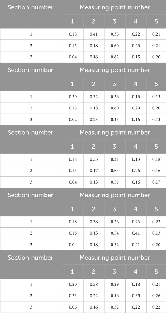
Table 4. Flow velocity (m/s) of measurement point at different depth (the measuring point is 18 cm from the height of the bottom of the pool) in pool room.

To assess boundary effects, vertical seam velocities were measured at multiple heights along middle baffle plates (Figure 17). The experimental data show an average velocity of 0.73 m/s across the vertical seam section, compared to the numerically predicted average of 0.68 m/s in Section 1 (upper, middle, and bottom layers). The 8% discrepancy between experimental and numerical results confirms the model’s capability to accurately represent actual flow conditions.

Figure 17

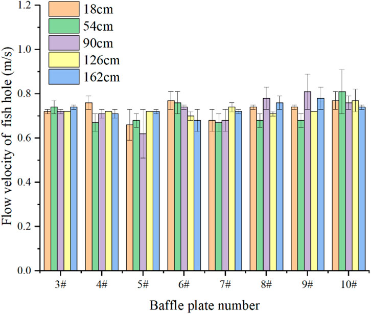
Figure 17. Flow velocity of each fish hole measurement point of the middle baffle plate.

5 Conclusion

This study developed a mathematical model of L-type baffle fishways based on the k-ε turbulence model, with numerical solutions obtained through the finite volume method, complemented by physical model experiments to systematically investigate its hydraulic characteristics and ecological benefits:

The L-type baffle generates a distinctive S-shaped main flow pattern, significantly reducing flow turbulence compared to conventional H-type baffles. The velocity distribution in critical zones precisely matches the passage requirements of the “Four Major Chinese Carps” (black carp, grass carp, silver carp, and bighead carp): the maximum velocity at vertical slots remains below the critical swimming speed (0.87 m/s vs. 1.3 m/s threshold), while the average slot velocity (0.50–0.77 m/s) optimally covers the target species’ preferred range (0.2–0.8 m/s).

The velocity distribution fully satisfies the swimming capacity requirements of these carps. Over 50% of the chamber area maintains low-velocity zones (<0.3 m/s), with bilateral recirculation zones exhibiting stable velocities below 0.2 m/s (approaching fish response thresholds). This configuration provides extensive resting areas (>85% of passage duration availability) while preventing juvenile displacement by high-velocity flows.

Physical experiments following Froude similarity principles demonstrated strong agreement with numerical predictions: the measured average slot velocity (0.73 m/s) showed <8% deviation from simulated values (0.68 m/s), while the S-shaped flow trajectory and low-velocity zone distribution exhibited >90% spatial consistency, validating the model’s predictive accuracy under complex boundary conditions.

The L-type baffle design criteria have been successfully implemented at the Zhuzhou Hub fishway, addressing spatial constraints in urban reaches. Its low-turbulence flow regime reduces fish migration energy expenditure by >30%, providing robust theoretical and practical guidance for optimizing fishway designs to enhance migratory success (25%–40% improvement) and ecological sustainability in regulated rivers.

Data availability statement

The raw data supporting the conclusions of this article will be made available by the authors, without undue reservation.

Author contributions

YL: Writing – original draft, Formal Analysis, Methodology, Conceptualization, Validation. JT: Supervision, Writing – review and editing, Methodology, Conceptualization, Visualization, Funding acquisition, Validation, Project administration. BL: Methodology, Validation, Investigation, Conceptualization, Writing – original draft. NW: Resources, Writing – original draft. YY: Writing – review and editing, Visualization. JM: Writing – original draft, Data curation.

Funding

The author(s) declare that financial support was received for the research and/or publication of this article. This research was funded by Hunan transportation science and technology project grant number (201543) and the APC was funded by Department of Transportation of Hunan Province in this section.

Acknowledgments

We the thank Nanjing Hydraulic Research Institute for providing us with a physical model testing site.

Conflict of interest

Authors YL, JT, NW, YY, and JM were employed by Hunan Province Communications Planning, Survey and Design Institute Co., Ltd.

The remaining author declares that the research was conducted in the absence of any commercial or financial relationships that could be construed as a potential conflict of interest.

Generative AI statement

The author(s) declare that no Generative AI was used in the creation of this manuscript.

Any alternative text (alt text) provided alongside figures in this article has been generated by Frontiers with the support of artificial intelligence and reasonable efforts have been made to ensure accuracy, including review by the authors wherever possible. If you identify any issues, please contact us.

Publisher’s note

All claims expressed in this article are solely those of the authors and do not necessarily represent those of their affiliated organizations, or those of the publisher, the editors and the reviewers. Any product that may be evaluated in this article, or claim that may be made by its manufacturer, is not guaranteed or endorsed by the publisher.

References

Abdolahipour, S. (2024). Review on flow separation control: effects of excitation frequency and momentum coefficient. Front. Mech. Eng. 10, 1380675. doi:10.3389/fmech.2024.1380675

CrossRef Full Text | Google Scholar

Ahmadi, M., Ghaderi, A., MohammadNezhad, H., Kuriqi, A., and Di Francesco, S. (2021). Numerical investigation of hydraulics in a vertical slot fishway with upgraded configurations. Water 13, 2711. doi:10.3390/w13192711

CrossRef Full Text | Google Scholar

Bai, R., Liu, X., Liu, X., Liu, L., Wang, J., Liao, S., et al. (2017). The development of biodiversity conservation measures in China’s hydro projects: a review. Environ. Int. 108, 285–298. doi:10.1016/j.envint.2017.09.007

PubMed Abstract | CrossRef Full Text | Google Scholar

Bermudez, M., Puertas, J., Cea, L., Pena, L., and Balairon, L. (2010). Influence of pool geometry on the biological efficiency of vertical slot fishways. Ecol. Eng. 36, 1355–1364. doi:10.1016/j.ecoleng.2010.06.013

CrossRef Full Text | Google Scholar

Bomba, M., Cetina, M., and Novak, G. (2017). Study on flow characteristics in vertical slot fishways regarding slot layout optimization. Ecol. Eng. 107, 126–136. doi:10.1016/j.ecoleng.2017.07.008

CrossRef Full Text | Google Scholar

Dong, M., Zeng, G., Xu, M., Mou, J., and Gu, Y. (2024). Influence of valvular structures on the flow characteristics in an island-type fishway. Water 16, 2336. doi:10.3390/w16162336

CrossRef Full Text | Google Scholar

Francisco Fuentes-Perez, J., Javier Sanz-Ronda, F., Martinez de Azagra, A., and Garcia-Vega, A. (2016). Non-uniform hydraulic behavior of pool-weir fishways: a tool to optimize its design and performance. Ecol. Eng. 86, 5–12. doi:10.1016/j.ecoleng.2015.10.021

CrossRef Full Text | Google Scholar

Kim, J. H. (2001). Hydraulic characteristics by weir type in a pool-weir fishway. Ecol. Eng. 16, 425–433. doi:10.1016/S0925-8574(00)00125-7

CrossRef Full Text | Google Scholar

Liu, J., Kattel, G., Wang, Z., and Xu, M. (2019). Artificial fishways and their performances in China’s regulated river systems: a historical synthesis. J. Ecohydraul 4, 158–171. doi:10.1080/24705357.2019.1644977

CrossRef Full Text | Google Scholar

Puertas, J., Pena, L., and Teijeiro, T. (2004). Experimental approach to the hydraulics of vertical slot fishways. J. Hydraul. Eng. 130, 10–23. doi:10.1061/(ASCE)0733-9429(2004)130:1(10)

CrossRef Full Text | Google Scholar

Qi, S., Fu, C., and Xie, M. (2024). Analysis of two-dimensional hydraulic characteristics of vertical-slot, double-pool fishway based on fluent. Water 16, 1695. doi:10.3390/w16121695

CrossRef Full Text | Google Scholar

Quaranta, E., Katopodis, C., and Comoglio, C. (2019). Effects of bed slope on the flow field of vertical slot fishways. River Res. Appl. 35, 656–668. doi:10.1002/rra.3428

CrossRef Full Text | Google Scholar

Romao, F., Branco, P., Quaresma, A. L., Amaral, S. D., and Pinheiro, A. N. (2018). Effectiveness of a multi-slot vertical slot fishway versus a standard vertical slot fishway for potamodromous cyprinids. Hydrobiologia 816, 153–163. doi:10.1007/s10750-018-3580-5

CrossRef Full Text | Google Scholar

Santos, J. M., Branco, P., Katopodis, C., Ferreira, T., and Pinheiro, A. (2014). Retrofitting pool-and-weir fishways to improve passage performance of benthic fishes: effect of boulder density and fishway discharge. Ecol. Eng. 73, 335–344. doi:10.1016/j.ecoleng.2014.09.065

CrossRef Full Text | Google Scholar

Sheikholeslam Noori, S. M., Taeibi Rahni, M., and Shams Taleghani, S. A. (2019). Multiple-relaxation time color-gradient lattice boltzmann model for simulating contact angle in two-phase flows with high density ratio. Eur. Phys. J. Plus 134, 399. doi:10.1140/epjp/i2019-12759-x

CrossRef Full Text | Google Scholar

Silva, A. T., Lucas, M. C., Castro-Santos, T., Katopodis, C., Baumgartner, L. J., Thiem, J. D., et al. (2018). The future of fish passage science, engineering, and practice. Fish. Fish. 19, 340–362. doi:10.1111/faf.12258

CrossRef Full Text | Google Scholar

Yu, Y., and Chang, J. (2025). Preliminary analysis of the construction and operation status of fish passage facility in China. Ecol. Eng. 212, 107515. doi:10.1016/j.ecoleng.2025.107515

CrossRef Full Text | Google Scholar

Yuan, H., Chen, B., Sun, Q., Xie, C., and He, X. (2024). Deciphering the effect of variation in slope on flow characteristics in a vertical slot fishway. J. Hydro-environ. Res. 54, 1–12. doi:10.1016/j.jher.2024.02.005

CrossRef Full Text | Google Scholar