Risk-aware local traffic safety evaluation for autonomous new energy vehicles based on virtual force modeling

Introduction: Ensuring safe driving and effective risk control is critical for the dynamic operation of autonomous new energy vehicles (NEVs), particularly under complex traffic conditions. A key challenge lies in unifying risk assessment across diverse driving scenarios, which hinders reliable and adaptive risk management in autonomous systems.

Methods: To address this challenge, a local traffic risk evaluation framework tailored for NEVs is proposed, grounded in the principle of least action. The method constructs a virtual force system centered on the autonomous NEV, integrating three components: (1) virtual risk force to capture vehicle-to-vehicle interaction risks; (2) virtual driving force reflecting the vehicle’s motion intention; and (3) virtual regulatory force to enforce traffic rule compliance. By modeling the action of this force system, a novel metric for local traffic safety is formulated, enabling real-time risk assessment and informing control strategies.

Results: The proposed method was validated through simulations across typical hazardous scenarios, including rear-end collisions, emergency deceleration, lane changes, and intersection conflicts. Simulations demonstrated that the framework enables timely risk perception and adaptive control behaviors (e.g., braking, evasive lane changes), which substantially improved the driving safety of NEVs.

Discussion: This work provides a unified and computationally efficient tool for enhancing risk-aware decision-making and control in autonomous NEVs. By addressing the challenge of scenario-unified risk assessment, it contributes to the safer deployment of autonomous NEVs and their more intelligent integration into traffic systems.

1 Introduction

The rapid development of autonomous driving technology is reshaping the future of transportation, with new energy vehicles (NEVs) emerging as a key platform for its implementation. By integrating electrification with intelligent driving systems, autonomous NEVs offer a sustainable and efficient mobility solution. Compared to conventional internal combustion engine vehicles, NEVs benefit from inherently abundant electrical power, which provides a favorable foundation for supporting the high energy demands of autonomous driving systems, including onboard sensors, computing units, and communication modules. Equipped with sophisticated perception, planning, and control algorithms, autonomous NEVs are designed to operate with minimal human input in complex and dynamic traffic environments. Nevertheless, ensuring safe and reliable autonomous operation across diverse real-world driving scenarios remains a significant challenge. The variability of road geometries, unpredictable behavior of other road users, and complex vehicle interactions call for robust and adaptive safety evaluation frameworks. In this context, accurately assessing local driving risks and enabling risk-aware decision-making are critical to enhancing the safety performance of autonomous NEVs and facilitating their large-scale deployment (Gao et al., 2022; Lu et al., 2022).

Evaluating the safety of a vehicle’s actions is a complex task due to the variety of scenarios an autonomous vehicle may encounter. Each scenario—lane changes, following another vehicle, or navigating through intersections—requires specific safety metrics to assess the risks involved accurately. For example, we evaluate lane-change scenarios using the available gap for a safe transition (Chen et al., 2021; Liu et al., 2021), assess car-following scenarios using metrics such as time to collision (TTC), inverse TTC, time-exposed TTC, time-integrated TTC, and time headway (THW) (Mao et al., 2021; Son et al., 2021; Li et al., 2022; Zhang et al., 2022), and evaluate intersection scenarios based on time to intersection (TTI). These metrics are often discrete and context-specific, making developing a unified safety evaluation method challenging.

The indicators mentioned in longitudinal and lateral contexts represent safety distance methods grounded in vehicle kinematics theory, incorporating both space and time dimensions. These methods primarily calculate driving risk through the vehicle’s state information and the relative motion between two vehicles. The simplicity and physical relevance of the parameters, which closely align with a driver’s intuitive understanding of safety, have made these methods widely used.

However, the rapid advancement of sensors, communication, and intelligent transportation technologies necessitates a breakthrough in critical technologies to advance intelligent vehicles beyond Level 2 (L2) and into Level 3 (L3) and higher levels of autonomous driving. Most current methods only apply to developing intelligent driving technology at Level 2 and below.

Researchers have recently developed quantitative risk assessment methods based on the artificial potential field (APF). They use APF as a typical two-dimensional driving risk assessment approach, incorporating longitudinal and lateral indicators to describe the relationship and risk levels between vehicles and their surrounding environment. This method is now being applied to research on intelligent vehicle safety algorithms.

The APF method, originally introduced by Khatib and Le Maitre (1978) in 1978 for robot control, has since evolved to describe driving risk levels. Researchers from institutions such as Drexel University (Bhatt et al., 1987) and the Georgia Institute of Technology (Arkin and Murphy, 1990) have applied APF to analyze the risk environment for autonomous vehicles. Gerdes and Rossetter (2001) advanced this by creating a risk distribution map and a unified driving assistance system based on APF. Matsumi et al. (2013) used APF to prevent vehicle collisions with pedestrians at intersections and protect vulnerable road users. Huang et al. (2021) developed a dynamic potential field for vehicle decision-making and motion planning using the APF model. Despite these advancements, the application scenarios for APF-based methods remain limited, and the model’s adaptability needs improvement. While APF theory matures and effectively assesses driving risk in areas like car following, path planning, and collision avoidance, previous studies have often overlooked critical factors. These include the driver’s psychological, physiological, and behavioral traits, complex weather and road conditions, and the interaction of various factors within the driver-vehicle-road system. To enhance driving safety assessments, Wang et al. (2016) proposed the “driving safety field (DSF)” model, which considers a comprehensive set of driver, vehicle, and road factors. However, the DSF model faces challenges in establishing a clear physical meaning for the coupling relationships between parameters.

In summary, several studies have been conducted on driving risk assessments, but various deficiencies exist. In this study, we construct a virtual force system from the perspective of autonomous vehicles, presenting a local traffic safety assessment method based on the principle of least action. The main contributions of this study are as follows:

(1) Established a virtual force system centered on the autonomous vehicle that incorporates virtual risk forces, virtual driving forces, and virtual traffic regulation constraint forces.

(2) Established a virtual risk force that satisfies Newton’s Third Law, achieving $F_{ji}=-F_{ij}$ while avoiding the scenario where the virtual risk force value is zero because the two vehicles are relatively stationary.

(3) Proposed a local traffic safety instantaneous evaluation index to achieve unified risk assessment across different driving scenarios.

The remainder of this article is organized as follows. Section 2 analyzes the driving process and establishes a physical model of vehicle motion. In Section 3, we study the virtual force system from the perspective of autonomous vehicles. According to the proposed virtual force system, we set up a local traffic safety assessment method in Section 4. In Section 5, we applied the established method in hazard scenarios by MATLAB’s Driving Scenario Designer to verify the effectiveness of the proposed model. In Section 6, we conclude this study.

2 The physical model of vehicle motion

The vehicle is influenced by three aspects of the driver-vehicle-road closed-loop system during driving: (1) the driver’s driving goals, (2) the impact of the dynamic traffic environment, and (3) the constraints imposed by traffic regulations. Based on this concept, we can vividly describe the driving process as a small ball rolling down from the top of a U-shaped groove, as shown in Figure 1.

Figure 1

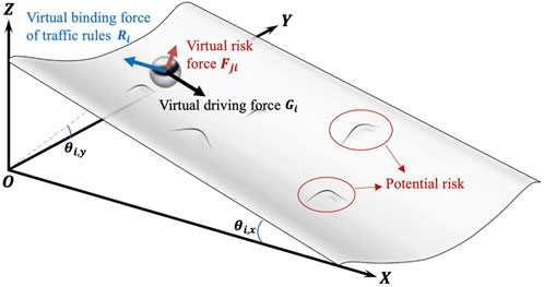
Figure 1. The physical model of vehicle motion.

As shown in Figure 1, the ball is subject to three types of forces during its downward rolling: (1) a virtual driving force driven by the driving target; (2) a virtual risk external force influenced by the dynamic traffic environment; (3) a virtual constraint resistance generated by traffic rules. In addition, the inclination angle of the U-shaped groove relates to the driver’s expected speed or expectation of mobility. The ball moves longitudinally when ${\theta }_{i,x}\ne 0$, corresponding to straight driving. The ball moves laterally when ${\theta }_{i,y}\ne 0$, corresponding to lane changing. The angle ${\theta }_i$ between the U-shaped groove and the XOY plane reflects the driver’s overall pursuit of efficiency. At the same time, ${\theta }_{i,x}$ and ${\theta }_{i,y}$ correspond to the driver’s pursuit of efficiency in the longitudinal and lateral directions during driving, respectively. According to the principle of Euler angle coordinate system transformation, the relationship between the above three parameters satisfies the following formula:

${\theta }_i=\arccos \left(\cos {\theta }_{i,x}·\cos {\theta }_{i,y}\right)(1)$

We define the virtual driving force as $G_i$, and let $G_i=m_{i}g\sin {\theta }_i$. In addition, drivers will inevitably encounter risk scenarios such as obstacles appearing ahead and neighboring vehicles forcibly cutting in while driving. This study describes the risk scenarios as small protrusions in a U-shaped groove, as marked by red circles in Figure 1, and represents them with virtual risk force $F_{ji}$. Furthermore, due to the existence of traffic rules (such as speed limits), drivers always avoid violating regulations while driving. Therefore, $R_i$ represents the virtual constraint resistance imposed by traffic rules on drivers.

3 Virtual force system from the perspective of autonomous vehicles

This study constructs a virtual force system from the perspective of autonomous vehicle $i$ (hereinafter referred to as vehicle $i$) to investigate the safety of the local road traffic environment surrounding autonomous vehicles. As shown in Figure 2, the white vehicle represents the autonomous vehicle $i$, surrounded by four brown vehicles, $j_1$, $j_2$, $j_3$, and $j_4$. These four surrounding vehicles exert virtual risk forces on vehicle $i$, denoted as $F_{j_{1}i}$, $F_{j_{2}i}$, $F_{j_{3}i}$, and $F_{j_{4}i}$, respectively. The virtual driving force corresponding to vehicle $i$'s driving intent is $G_i$. The road speed limit rule imposes a virtual constraint force on vehicle $i$'s behavior, denoted as $R_{si}$. Additionally, the constraints from the lane lines on both sides of vehicle $i$ are represented as $R_{l_{1}i}$ and $R_{l_{2}i}$. The following sections will provide a detailed introduction to modeling these virtual forces in the local road traffic environment for autonomous vehicles.

Figure 2

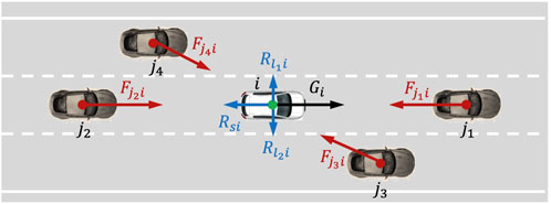
Figure 2. Virtual force system from the perspective of autonomous vehicles.

3.1 Virtual risk forces

We proposed the basic driving-risk-field force model in the previous study by analyzing the relationship between force work and energy conversion in the collision process (Zheng et al., 2024). That is,

$F_{ji}=\left\{\begin{array}{ll}{E}_j/r_e& r_{ji}\in [0,r_{\min })\\ E_j{r}_0\left(\frac{1}{r_{ji}^2}-\frac{1}{r_{\max }^2}\right)& r_{ji}\in \left[r_{\min },r_{\max }\right]\\ 0& r_{ji}\in \left(r_{\max },+\infty \right)\end{array}\right.(2)$

Where $E_j$ denotes the kinetic energy of vehicle $j$, $r_{ji}^2=k_x{x}_{ji}^2+k_y{y}_{ji}^2$, $k_x$ and $k_y$ are the longitudinal and lateral gradient coefficients of risk, while $x_{ji}$ and $y_{ji}$ are the longitudinal and transverse relative distances between vehicle $j$ and $i$ in the vehicle $j$ coordinate system, respectively. $R_e$ is the unit length, that is, $r_e=1\mathrm{m}$; $r_{\max }$ is the distance between free-flowing vehicles, used to represent the maximum impact range of risk. The value of $r_{\min }$ is used to determine the inflection point of the segmented function of $F_{ji}$. $r_0$ is the driver’s scope of attention to risk. The values of $r_0$, $r_{\max }$, and $r_{\min }$ refer to our previous research (Zheng et al., 2024).

We analyze the vehicle-to-vehicle interaction to quantify the risk between two moving objects in space, as shown in Figure 3. Vehicles $i$ and $j$ are moving with vector velocities ${\mathit{v}}_{\mathit{i}}$ and ${\mathit{v}}_{\mathit{j}}$, respectively. The relative velocity between the two vehicles is ${\mathit{v}}_{\mathit{j}\mathit{i}}$. If we use the position of vehicle $j$ as the origin and establish a coordinate axis $x^j$ in the direction of the relative velocity ${\mathit{v}}_{\mathit{j}\mathit{i}}$, and a perpendicular coordinate axis $y^j$, then ${\theta }_{ji}$ represents the angle between ${\mathit{v}}_{\mathit{j}\mathit{i}}$ and the line $d_{ji}$ connecting vehicles $j$ and $i$. Clearly, the smaller ${\theta }_{ji}$ is, the greater the risk that vehicle $i$ faces from vehicle $j$. The angle ${\theta }_{ji}$ depends on the positions and velocities of the two vehicles.

Figure 3

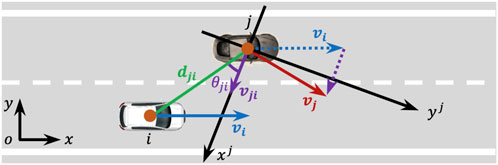
Figure 3. Vehicle-to-vehicle interaction schematic diagram.

To achieve $F_{ji}=-F_{ij}$ while also addressing the situation where the virtual risk force value is zero because the two vehicles are relatively stationary, we modify the model shown in Equation 2 as follows:

$F_{ji}=\left\{\begin{array}{cc}\frac{1}{2}{M}_{ji}{V}_{ji}^2/r_e& r_{ji}^{\prime }\in [0,r_{\min })\\ \frac{1}{2}{M}_{ji}{V}_{ji}^2{r}_0\left(\frac{1}{r_{ji}^{\prime 2}}-\frac{1}{r_{\max }^2}\right)& r_{ji}^{\prime }\in \left[r_{\min },r_{\max }\right]\\ 0& r_{ji}^{\prime }\in \left(r_{\max },+\infty \right)\end{array}\right.(3)$

where, M_ji, V_ji and r_ji′ can be expressed as Equations 4–6

$M_{ji}=\frac{m_i{m}_j}{m_i+m_j}(4)$

$V_{ji}=\sqrt{{\overline{\mathit{v}}}_{\mathit{j}\mathit{i}}^2+{\mathit{v}}_{\mathit{j}\mathit{i}}^2}(5)$

$r_{ji}^{\prime }=\sqrt{k_x{x}_i^{\prime 2}+k_y{y}_i^{\prime 2}}(6)$

$M_{ji}$ represents the reduced mass of vehicles $i$ and $j$; $m_i$ and $m_j$ are the masses of vehicles $i$ and $j$, respectively; ${\overline{\mathit{v}}}_{\mathit{j}\mathit{i}}^2$ is the average speed of vehicles $i$ and $j$; $x_i^{\prime }$ and $y_i^{\prime }$ are the coordinates of vehicle $i$ in the $x^{j}j{y}^j$ coordinate system; $r_0$ is the driver’s following distance.

If the actual geographical coordinates of the vehicles $j$ and $i$ are $\left(x_j,y_j\right)$ and $\left(x_i,y_i\right)$, respectively, and ${\theta }_j$ is the rotation angle of the coordinate system, then the coordinates of the vehicle $i$ in the $x^{j}j{y}^j$ coordinate system are

$\left[\begin{array}{c}{x}_i^{\prime }\\ y_i^{\prime }\\ 1\end{array}\right]=\left[\begin{array}{ccc}\cos {\theta }_j& -\sin {\theta }_j& 0\\ \sin {\theta }_j& \cos {\theta }_j& 0\\ 0& 0& 1\end{array}\right]\left[\begin{array}{ccc}1& 0& -x_j\\ 0& 1& -y_j\\ 0& 0& 1\end{array}\right]\left[\begin{array}{c}{x}_i\\ y_i\\ 1\end{array}\right](7)$

3.2 Virtual driving force

The virtual driving force causes vehicle $i$ to move from the starting to the end position. When there is no lane-changing process, the target driving force of vehicle $i$ exists only in the longitudinal direction; when lane-changing occurs due to the lateral movement, the target driving force of vehicle $i$ will have a component in the lateral direction. The overall virtual driving force satisfies the following:

$G_i=m_{i}g\sin {\theta }_i(8)$

3.2.1 Longitudinal driving force

The virtual force $G_i$ represents the driver’s demand for maneuverability. According to the physical model shown in Figure 1, during the straight driving process without lane-changing behavior, ${\theta }_{i,y}=0$. Therefore, according to Equation 1, ${\theta }_i={\theta }_{i,x}$, and the virtual force acting on vehicle $i$ can be expressed by Equation 9:

$G_{i,x}=m_{i}g\sin {\theta }_{i,x}(9)$

where $m_i$ is the mass of vehicle $i$; $g$ is the gravitational acceleration; ${\theta }_i$ is the tilt angle of the U-shaped groove in the physical model, which is related to the vehicle $i$'s pursuit of driving speed. In this article, ${\theta }_i$ is defined to satisfy Equation 10:

$\sin {\theta }_{i,x}=k\frac{v_{der}}{v_l}(10)$

where $k$ is a constant, set to $k=0.2$ in this study; $v_{der}$ is the desired speed of vehicle $i$; $v_l$ is the speed limit of the lane.

3.2.2 Lateral driving force

When vehicle $i$ intends to change lanes, the virtual driving force $G_i$ acting on vehicle $i$ under the driving target will generate two components in the longitudinal and lateral directions of the vehicle, as shown in Figure 1. Vehicle $i$ is subjected to virtual attractive forces $G_{i,x}$ and $G_{i,y}$ in the longitudinal and lateral directions, respectively. Based on Equation 1 and the principle of Euler angle coordinate system transformation, we calculate G_i,x and G_i,y use Equations 11, 12

$G_{i,x}=m_{i}g\sin {\theta }_i·\cos {\theta }_{i,y}(11)$

$G_{i,y}=m_{i}g\sin {\theta }_i·\sin {\theta }_{i,y}(12)$

${\theta }_{i,x}$ is related to the driving expectation of vehicle $i$ in the longitudinal direction. Similarly, ${\theta }_{i,y}$ is related to the lateral lane-changing behavior of vehicle $i$. When the driver intends to change lanes, the first step is to overcome the constraint imposed by the lane line on the vehicle and move toward the centerline of the target lane. Therefore, similar to Equation 10, we define θ_i,y as Equation 13

${\theta }_{i,y}=\arcsin \left(k_{ic}\frac{d_{i,aim}}{l_w}\right)(13)$

where $d_{i,aim}$ is the distance between vehicle $i$ and the centerline of the target lane; $l_w$ is the lane width, set to $l_w=3.5$ meters; $k_{ic}$ is a constant.

3.3 Virtual traffic regulation constraint force

Traffic rules impose various constraints on vehicles, such as traffic lights, pedestrian crossings, speed limit signs, and road markings, which can restrict vehicle movement. In this study, we consider only the longitudinal constraint on vehicle movement due to road speed limit signs and the lateral constraint due to road markings.

3.3.1 Longitudinal constraint resistance

Because road speed limit rules are effective everywhere on the road they pertain to, the constraint is only related to speed. If the vehicle $i$ stops, that is, when $v_i=0$, the constraint resistance $R_i=0$; if the vehicle $i$ accelerates to the road speed limit, that is, when $v_i=v_{limit}$, the virtual constraint resistance equals the virtual driving force, that is, $R_i=G_i$. Therefore, the virtual constraint resistance $R_i$ is designed to satisfy the following equation:

$R_i=m_{i}g\sin {\theta }_{i,x}\frac{v_i}{v_l}(14)$

where $v_i$ is the speed of vehicle $i$; $v_l$ is the road speed limit. Equation 14 shows that the closer the vehicle speed is to the road speed limit, the greater the constraint resistance.

3.3.2 Lateral constraint resistance

Road traffic markings include white dashed/solid lines, double white dashed/solid lines, yellow dashed/solid lines, and double yellow dashed/solid lines. Each type of road traffic marking has different meanings and serves to constrain the risks associated with vehicle operation. This study focuses on the white dashed lines painted on road segments to separate traffic flows traveling in the same direction, commonly called lane lines. Research has shown that wider lanes are not necessarily safer; setting narrower lanes, although typically causing vehicles to travel at slower speeds, can make drivers more focused and thereby reduce the probability of traffic accidents (Godley et al., 2004; Potts et al., 2007; Labi et al., 2017). This indicates that road traffic markings play a role in guiding and constraining driving behavior. Lane markings influence the lateral behavior of vehicles. Road traffic markings do not directly affect the risk of vehicle operation, and vehicles do not cause traffic accidents solely by crossing road traffic markings. Typically, road traffic markings are seen as providing a virtual constraint (such as lane keeping) on the lateral movement of vehicles during their operation (Gerdes et al., 2001; Rossetter et al., 2004; Rossetter and Gerdes, 2005; Talvala et al., 2011). In this study, the constraint imposed by road traffic markings on vehicles is defined as Equation 15

$F_{li}=\frac{k_m{E}_i}{k_y}\left(\frac{1}{y_{mi}+y_p}-y_p\right)(15)$

where $k_m$ is a constant coefficient, set to $k_m=0.1$; $k_y$ is the lateral gradient adjustment coefficient; $y_{mi}$ represents the lateral distance between vehicle $i$ and lane line $m$, with no effect from traffic markings when the vehicle is driving on the lane centerline; $y_p$ represents the offset, set to $y_p=-0.5l_w+\left(\sqrt{0.25l_w^2+l_0}\right)$, where $l_0$ represents the width of a lane, take $l_0=4\mathrm{m}$.

A comprehensive system is established by modeling virtual forces in the local road traffic environment of autonomous vehicles, integrating vehicle motion, traffic regulations, and risks from other vehicles. The following sections will conduct safety assessment research on the local road traffic environment under this virtual force system framework.

4 Local traffic safety assessment methods

In the virtual force system established from the perspective of autonomous vehicles in Section 3, we can analyze the driving safety of autonomous vehicles in the local traffic environment using the principle of minimum action (Wang et al., 2020; Zheng et al., 2021). First, as shown in Figure 2, centered around autonomous vehicle $i$, we calculate the potential energy exerted on vehicle $i$ by the virtual risk force, virtual driving force, and virtual regulatory constraint force. The virtual risk force generates virtual risk potential energy, which describes the risk situation during the driving process. The greater the virtual risk potential energy, the higher the driving risk. Conversely, the virtual driving force and virtual regulatory constraint force generate virtual driving potential energy, which describes the efficiency of the driving process. The greater the virtual driving potential energy, the lower the efficiency. Therefore, the lower the total potential energy of the vehicle $i$, the safer and more efficient it is calculated as Equation 16.

Based on Equation 3, the virtual risk potential energy $U_{F_{ji}}$ caused by any other road user on vehicle $i$ is calculated as Equation 16.

$U_{F_{ji}}=\left\{\begin{array}{cc}\frac{1}{2}{M}_{ji}{V}_{ji}^2{R}_1& r_{ji}^{\prime }\in [0,r_{\min })\\ \frac{1}{2}{M}_{ji}{V}_{ji}^2{R}_2& r_{ji}^{\prime }\in \left[r_{\min },r_{\max }\right]\\ 0& r_{ji}^{\prime }\in \left(r_{\max },+\infty \right)\end{array}\right.(16)$

where the expressions for R₁ and R₂ are as Equations 17–18.

$R_1=\left(r_{\min }-r_{ji}^{\prime }\right)/r_e+r_0\left(\frac{1}{r_{\min }}+\frac{r_{\min }-2r_{\max }}{r_{\max }^2}\right)(17)$

$R_2=r_0\left(\frac{1}{r_{ji}^{\prime }}+\frac{r_{ji}^{\prime }-2r_{\max }}{r_{\max }^2}\right)(18)$

Therefore, the total virtual risk potential energy $U_F$ exerted on vehicle $i$ by $n$ other road users in the environment is obtained by Equation 19.

$U_F=\sum _{j=1}^n{U}_{F_{ji}}(19)$

For simplicity, when modeling the virtual driving potential energy $U_G$ generated by the longitudinal virtual driving force and virtual regulatory constraint force, because ${\theta }_i$ and ${\theta }_{ix}$ are relatively close, we consider ${\theta }_i\approx {\theta }_{ix}$. Combining Equations 8, 14, we obtain U_G by using Equation 20.

$U_G=m_{i}g{\sin \theta }_i\frac{{\left(v_l-v_i\right)}^2}{{2v}_l}{t}_e(20)$

where $t_e$ is the unit time.

At the same time, ignoring the influence of $G_{i,y}$, the virtual constraint potential energy $U_R$ generated by the lateral virtual regulatory constraint force is given by Equation 21.

$U_R=\frac{k_m{E}_i}{k_y}\left(\ln \frac{y_{mi}-y_p}{y_p}-y_p{y}_{mi}\right)t_e(21)$

Therefore, in the virtual force system centered around vehicle $i$, the total potential energy $U_i$ experienced by vehicle $i$ in any given scenario is calculated by Equation 22.

$U_i=U_F+U_G+U_R(22)$

According to the principle of minimum action, the action equation for the virtual force system centered around vehicle $i$ is constructed as follows as Equation 23.

$S={\int }_{t_0}^{t_f}Ldt(23)$

where $S$ is the action of the driving process of vehicle $i$. Because the virtual force system is centered around vehicle $i$, $T_i=0$, and the Lagrangian $L$ is given by $L=T_i-U_i=-U_i$.

Theoretically, the lower the total potential energy of vehicle $i$, the safer and more efficient it is. When vehicle $i$ is driving along the lane centerline at the road speed limit in free flow, $U_F=U_G=U_R=0$, and the action $S=0$, achieving an extremum. This indicates that the vehicle’s driving state is the safest and most efficient. However, in most cases, vehicle $i$ will experience virtual risk forces from other vehicles and cannot always travel at the road speed limit. Therefore, under typical conditions, $S<0$. Thus, this study designs a local traffic safety instantaneous evaluation index $D$, as shown in Equation 24, such that $D=1$ when $S=0$, and $\left.D\in [0,1\right)$ when $S<0$.

$D=2-a^{\left|S\right|}(24)$

where $a$ is a constant, with $a\in \left(1,\sqrt[\left|S\right|]{2}\right]$.

5 Hazard scenario design and simulation analysis

Driving safety is influenced by the vehicle’s motion state. Any vehicle’s hazardous behavior will quickly impact adjacent vehicles’ safety and gradually affect the safety and efficiency of the entire traffic flow. In this section, we design various hazard scenarios from the perspective of autonomous vehicles to demonstrate the effectiveness of the proposed local traffic safety assessment method. These scenarios include rear-end scenarios, a cut-in scenario, and an intersection collision scenario. By calculating the absolute value of the action $\left|S\right|$ and the local traffic safety instantaneous evaluation index $D$ in different scenarios, we analyze the safety of autonomous vehicles during driving. This study ignores vehicle dimensions and uses point masses for calculations for ease of analysis.

Figure 4 shows the designed rear-end (collision) scenario, where autonomous vehicle $i$ and another vehicle $j$ are in the same lane, separated by 120 m. Vehicle $i$ travels at a speed of $30m/s$, and if the motion state remains unchanged, a rear-end collision will occur after 4 s. We use MATLAB’s Driving Scenario Designer to design and simulate the scenario, as shown in Figure 5. The results indicate that, over time, the absolute value of the action $\left|S\right|$ gradually increases, and the local traffic safety instantaneous evaluation index $D$ gradually decreases. A collision occurs after 4 s. If, during this process, autonomous vehicle $i$ detects the risk from vehicle $j$ in front and takes braking or lane-changing actions to avoid the risk, the absolute value of the action $\left|S\right|$ will not continue to increase, meaning the risk will not persist.

Figure 4

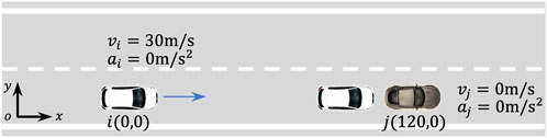
Figure 4. Rear-end (collision) scenario.

Figure 5

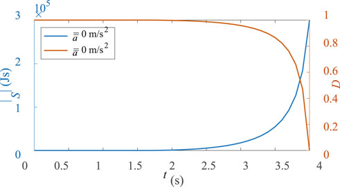
Figure 5. Instantaneous risk simulation results for the rear-end (collision) scenario.

First, we design a deceleration to avoid collision scenario with three different deceleration rates: $-4m/s2$, $-6m/s2$, and $-8m/s2$, representing gradual to emergency braking, as shown in Figure 6. To ensure comparability, we set the stopping position of vehicle $i$ to be the same in each case. We use MATLAB’s Driving Scenario Designer to create and simulate these scenarios, and the result is illustrated in Figure 7. In the legend, EB-1, EB-2, and EB-3 correspond to decelerations of $-4m/s2$, $-6m/s2$, and $-8m/s2$, respectively.

Figure 6

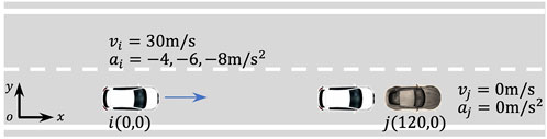
Figure 6. Rear-end (deceleration to avoid collision) scenario.

Figure 7

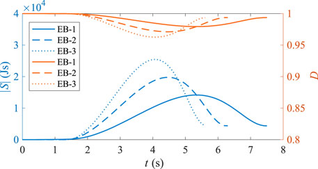
Figure 7. Instantaneous risk simulation results for the rear-end (deceleration to avoid collision) scenario.

From the figure, we can observe that due to the braking of vehicle $i$, the driving time increases from 4 s to 5.6 s, 6.3 s, and 7.5 s for the respective decelerations. Compared to the rear-end (collision) scenario, the absolute value of the action $\left|S\right|$ significantly decreases, and the local traffic safety instantaneous evaluation index $D$ substantially improves. Additionally, higher deceleration rates result in larger $\left|S\right|$, indicating higher risk, which aligns with practical observations.

To avoid rear-end collisions, in addition to braking to decelerate the vehicle, lane-changing can also be employed. Therefore, we designed a lane-change avoidance scenario, as shown in Figure 8. For comparison purposes, vehicle $i$ starts changing lanes at distances of 80 m, 60 m, and 40 m from vehicle $j$, with consistent lane-change trajectory curvature. We use MATLAB’s Driving Scenario Designer to design and simulate these scenarios, and the results are shown in Figure 9. In the legend, LC-1, LC-2, and LC-3 correspond to lane-change starting distances of 80 m, 60 m, and 40 m, respectively.

Figure 8

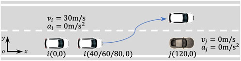
Figure 8. Rear-end (lane change to avoid collision) scenario.

Figure 9

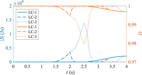
Figure 9. Instantaneous risk simulation results for the rear-end (lane change to avoid collision) scenario.

The figure shows that compared to the rear-end collision scenario, the absolute value of the action $\left|S\right|$ significantly decreases, and the local traffic safety instantaneous evaluation index $D$ shows a notable improvement. Additionally, the results indicate that a longer lane-change starting distance corresponds to greater safety, which aligns with practical observations.

When an obstacle is in front of the vehicle, the vehicle can change lanes to avoid rear-end collisions. However, if the vehicle is too close to other vehicles in the adjacent lane during the lane change, it can pose a risk. Therefore, we designed a cut-in scenario, as shown in Figure 10. For comparison, we designed vehicle $j$ to begin cutting in at distances of 10 m, 15 m, and 20 m from vehicle $i$, with consistent lane-change trajectory curvature. We used MATLAB’s Driving Scenario Designer to create and simulate these scenarios, and the results are shown in Figure 11. In the legend, CI-1, CI-2, and CI-3 correspond to cut-in starting distances of 5 m, 7.5 m, and 10 m, respectively.

Figure 10

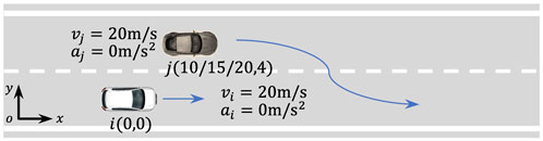
Figure 10. Cut-in scenario.

Figure 11

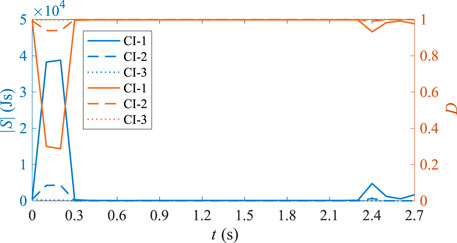
Figure 11. Instantaneous risk simulation results for the cut-in scenario.

The figure shows that the closer the initial distance between the two vehicles during the cut-in, the greater the risk, which aligns with practical observations. The results also indicate that a vehicle should maintain a sufficient longitudinal distance from vehicles in the adjacent lane before changing lanes.

Research (Zhao et al., 2019) indicates that traffic accidents at non-signalized intersections are generally more severe than those at signalized intersections, and advanced driving assistance systems, such as emergency braking systems, are ineffective in mitigating accidents at non-signalized intersections. Therefore, this study conducts a simulation analysis for non-signalized intersections.

First, we design a collision scenario at a non-signalized intersection, as shown in Figure 12. Vehicles $i$ and $j$ travel at a constant speed of $20m/s$ along their respective lanes. If the motion state remains unchanged, they will inevitably collide at point $C(2,-2$) after 2.5 s. We used MATLAB’s Driving Scenario Designer to create and simulate this scenario, and the results are shown in Figure 13.

Figure 12

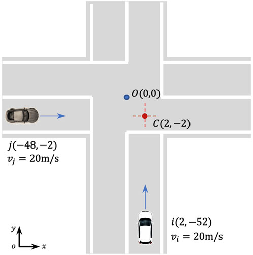
Figure 12. Non-signalized intersections (collision) scenario.

Figure 13

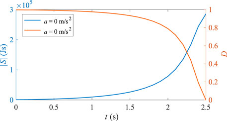
Figure 13. Instantaneous risk simulation results for the non-signalized intersection collision scenario.

The results reveal that as time progresses, the absolute value of the action $\left|S\right|$ gradually increases, and the local traffic safety instantaneous evaluation index $D$ gradually decreases, leading to a collision at 2.5 s. If, during this process, autonomous vehicle $i$ detects the risk from vehicle $j$ and takes braking actions to avoid the risk, the absolute value of the action $\left|S\right|$ will not continue to increase, meaning the risk will not persist.

Assume that autonomous vehicle $i$ detects vehicle $j$ when it is 10 m from the collision point and begins braking. We set the speeds of vehicle $i$ at the trajectory intersection point with vehicle $j$ to be $18m/s$, $16m/s$, and $14m/s$, as shown in Figure 14. We use MATLAB’s Driving Scenario Designer to design and simulate these scenarios, and the results are shown in Figure 15. In the legend, NSI-1, NSI-2, and NSI-3 correspond to the speeds of vehicle $i$ at the trajectory intersection point being 18 m/s, 16 m/s, and 14 m/s, respectively. The results indicate that when vehicle $i$ starts braking at point $\left(2,-12\right)$, that is, at simulation time $t=2$ seconds, the absolute value of the action $\left|S\right|$ gradually decreases, and the local traffic safety instantaneous evaluation index $D$ gradually increases. Additionally, the lower the speed of vehicle $i$ at the trajectory intersection point, the smaller the absolute value of the action $\left|S\right|$ and the higher the local traffic safety instantaneous evaluation index $D$, which aligns with practical observations.

Figure 14

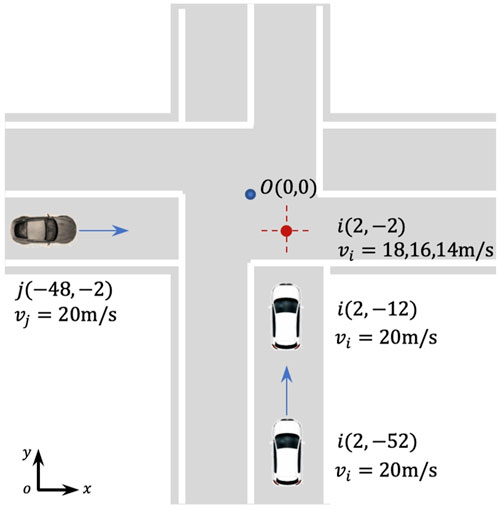
Figure 14. Non-signalized intersections (deceleration to avoid collision) scenario.

Figure 15

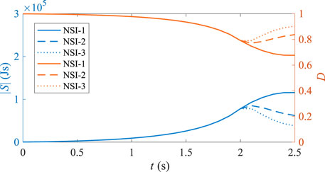
Figure 15. Instantaneous risk simulation results for the non-signalized intersections (deceleration to avoid collision) scenario.

6 Conclusion

In this study, we propose a local traffic safety evaluation method specifically designed for NEVs. By integrating a system of virtual forces to represent driving intentions, regulatory constraints, and interactive dynamics with surrounding vehicles, the method establishes a unified and real-time framework for evaluating driving safety under complex conditions. Through simulations of representative scenarios—including rear-end risks, emergency deceleration, lane changes, cut-ins, and intersection conflicts—the proposed approach effectively predicts and quantifies potential risks. Results demonstrate that timely hazard recognition and the execution of appropriate maneuvers, such as braking or evasive lane changes, substantially reduce local driving risk and enhance overall safety performance. The proposed evaluation framework offers critical support for the design and optimization of autonomous driving algorithms on NEV platforms, contributing to the development of safer, more adaptive, and energy-efficient intelligent transportation systems.

Data availability statement

The original contributions presented in the study are included in the article/supplementary material, further inquiries can be directed to the corresponding author.

Author contributions

HL: Writing – original draft and Writing – review and editing. YW: Data curation, Formal Analysis, Writing – original draft. JS: Software and Writing – original draft. XX: Supervision and Writing – review and editing.

Funding

The author(s) declare that financial support was received for the research and/or publication of this article. This work was supported by the Natural Science Foundation of Chongqing under Grant cstc2021jcyj-msxmX0708, in part by the Youth Project of Science and Technology Research Program of Chongqing Education Commission of China under Grant Nos. KJQN202303902 and KJQN202403905, and in part by the Chongqing City Vocational College Research Project under Grant No. XJKJ202301001.

Conflict of interest

The authors declare that the research was conducted in the absence of any commercial or financial relationships that could be construed as a potential conflict of interest.

Generative AI statement

The author(s) declare that no Generative AI was used in the creation of this manuscript.

Publisher’s note

All claims expressed in this article are solely those of the authors and do not necessarily represent those of their affiliated organizations, or those of the publisher, the editors and the reviewers. Any product that may be evaluated in this article, or claim that may be made by its manufacturer, is not guaranteed or endorsed by the publisher.

References

Arkin, R. C., and Murphy, R. R. (1990). Autonomous navigation in a manufacturing environment. IEEE Trans. Robotics Automation 6, 445–454. doi:10.1109/70.59355

CrossRef Full Text | Google Scholar

Bhatt, R., Gaw, D., and Meystel, A. (1987). “A real-time guidance system for an autonomous vehicle,” in 1987 IEEE international conference on robotics and automation proceedings, 1785–1791. doi:10.1109/ROBOT.1987.1087769

CrossRef Full Text | Google Scholar

Chen, D., Srivastava, A., and Ahn, S. (2021). Harnessing connected and automated vehicle technologies to control Lane changes at freeway merge bottlenecks in mixed traffic. Transp. Res. Part C Emerg. Technol. 123, 102950. doi:10.1016/j.trc.2020.102950

CrossRef Full Text | Google Scholar

Gao, F., Mu, J., Han, X., Yang, Y., and Zhou, J. (2022). Performance limit evaluation strategy for automated driving systems. Automot. Innov. 5, 79–90. doi:10.1007/s42154-021-00168-8

CrossRef Full Text | Google Scholar

Gerdes, J. C., and Rossetter, E. J. (2001). A unified approach to driver assistance systems based on artificial potential fields. Transactions-American Soc. Mech. Eng. J. Dyn. Syst. Meas. Control 123, 431–438. doi:10.1115/1.1386788

CrossRef Full Text | Google Scholar

Gerdes, J. C., Rossetter, E. J., and Saur, U. (2001). Combining lanekeeping and vehicle following with hazard maps. Veh. Syst. Dyn. 36, 391–411. doi:10.1076/vesd.36.4.391.3548

CrossRef Full Text | Google Scholar

Godley, S. T., Triggs, T. J., and Fildes, B. N. (2004). Perceptual Lane width, wide perceptual road centre markings and driving speeds. Ergonomics 47, 237–256. doi:10.1080/00140130310001629711

PubMed Abstract | CrossRef Full Text | Google Scholar

Huang, C., Lv, C., and Xing, Y. (2021). Toward safe and personalized autonomous driving: decision-making and motion control with DPF and CDT techniques. IEEE/ASME Trans. Mechatronics 26, 611–620. doi:10.1109/tmech.2021.3053248

CrossRef Full Text | Google Scholar

Khatib, O., and Le Maitre, J. F. (1978). “Dynamic control of manipulators operating in a complex environment,” in On theory and practice of robots and manipulators, 3rd CISM-IFToMM symp, 267–282. Available online at: http://www-cs.stanford.edu/group/manips/publications/pdfs/Khatib_1978.pdf.

Google Scholar

Labi, S., Chen, S., Preckel, P. V., Qiao, Y., and Woldemariam, W. (2017). Rural two-lane highway shoulder and Lane width policy evaluation using multiobjective optimization. Transp. A Transp. Sci. 13, 631–656. doi:10.1080/23249935.2017.1315841

CrossRef Full Text | Google Scholar

Li, Y., Lv, Q., Zhu, H., Li, H., Li, H., Hu, S., et al. (2022). Variable time headway policy based platoon control for heterogeneous connected vehicles with external disturbances. IEEE Trans. Intell. Transp. Syst. 23, 21190–21200. doi:10.1109/TITS.2022.3170647

CrossRef Full Text | Google Scholar

Liu, X., Wang, Y., Zhou, Z., Nam, K., Wei, C., and Yin, C. (2021). Trajectory prediction of preceding target vehicles based on Lane crossing and final points generation model considering driving styles. IEEE Trans. Veh. Technol. 70, 8720–8730. doi:10.1109/TVT.2021.3098429

CrossRef Full Text | Google Scholar

Lu, H., Lu, C., Yu, Y., Xiong, G., and Gong, J. (2022). Autonomous overtaking for intelligent vehicles considering social preference based on hierarchical reinforcement learning. Automot. Innov. 5, 195–208. doi:10.1007/s42154-022-00177-1

CrossRef Full Text | Google Scholar

Mao, S., Xiao, G., Lee, J., Wang, L., Wang, Z., and Huang, H. (2021). Safety effects of work zone advisory systems under the intelligent connected vehicle environment: a microsimulation approach. JICV 4, 16–27. doi:10.1108/JICV-07-2020-0006

CrossRef Full Text | Google Scholar

Matsumi, R., Raksincharoensak, P., and Nagai, M. (2013). Autonomous braking control system for pedestrian collision avoidance by using potential field. IFAC Proc. Vol. 46, 328–334. doi:10.3182/20130904-4-JP-2042.00064

CrossRef Full Text | Google Scholar

Potts, I. B., Harwood, D. W., and Richard, K. R. (2007). Relationship of Lane width to safety on urban and suburban arterials. Transp. Res. Rec. 2023, 63–82. doi:10.3141/2023-08

CrossRef Full Text | Google Scholar

Rossetter, E. J., and Gerdes, J. C. (2005). Lyapunov based performance guarantees for the potential field lane-keeping assistance system. J. Dyn. Sys., Meas. Control 128, 510–522. doi:10.1115/1.2192835

CrossRef Full Text | Google Scholar

Rossetter, E. J., Switkes, J. P., and Gerdes, J. C. (2004). Experimental validation of the potential field lanekeeping system. Int. J. Automot. Technol. 5, 95–108. Available online at: https://koreascience.kr/article/JAKO200411922949672.page

Google Scholar

Son, S., Park, J., Oh, C., and Yeom, C. (2021). An algorithm for detecting collision risk between trucks and pedestrians in the connected environment. J. Adv. Transp. 2021, 1–9. doi:10.1155/2021/9907698

CrossRef Full Text | Google Scholar

Talvala, K. L. R., Kritayakirana, K., and Gerdes, J. C. (2011). Pushing the limits: from lanekeeping to autonomous racing. Annu. Rev. Control 35, 137–148. doi:10.1016/j.arcontrol.2011.03.009

CrossRef Full Text | Google Scholar

Wang, J., Wu, J., Zheng, X., Ni, D., and Li, K. (2016). Driving safety field theory modeling and its application in pre-collision warning system. Transp. Res. Part C Emerg. Technol. 72, 306–324. doi:10.1016/j.trc.2016.10.003

CrossRef Full Text | Google Scholar

Wang, J., Zheng, X., and Huang, H. (2020). Decision-making mechanism of the drivers following the principle of least action. China J. Highw. Transp. 33, 155–168. doi:10.19721/j.cnki.1001-7372.2020.04.016

CrossRef Full Text | Google Scholar

Zhang, P., Zhu, B., Zhao, J., Fan, T., and Sun, Y. (2022). Performance evaluation method for automated driving system in logical scenario. Automot. Innov. 5, 299–310. doi:10.1007/s42154-022-00191-3

CrossRef Full Text | Google Scholar

Zhao, Z., Zheng, X., Wang, J., Xu, Q., and Kodaka, K. (2019). Assessing performance of collision mitigation brake system in Chinese traffic environment. J. Cent. South Univ. 26, 2854–2869. doi:10.1007/s11771-019-4219-z

CrossRef Full Text | Google Scholar

Zheng, X., Huang, H., Wang, J., Zhao, X., and Xu, Q. (2021). Behavioral decision-making model of the intelligent vehicle based on driving risk assessment. Computer-Aided Civ. Infrastructure Eng. 36, 820–837. doi:10.1111/mice.12507

CrossRef Full Text | Google Scholar

Zheng, X., Jiang, J., Huang, H., Wang, J., Xu, Q., and Zhang, Q. (2024). Novel quantitative approach for assessing driving risks and simulation study of its prevention and control strategies. J. Mech. Eng. 60, 207–221. doi:10.3901/JME.2024.10.207

CrossRef Full Text | Google Scholar