Robot fault prediction based on improved GM(1,1) model and RBF

Introduction: As the core equipment of intelligent manufacturing, the operational stability of industrial robots directly affects production efficiency and safety. However, long-term operation under complex working conditions can easily result in mechanical wear, electrical failures, and other issues, resulting in an average fault repair time of 4-8 hours.

Methods: A new hybrid prediction method combining the grey model and radial basis function is designed. The sensitivity problem of the grey model initial value is optimized through initial value correction, and the non-linear fitting ability of the neural network is combined. At the same time, the extreme value method is used to dynamically adjust weights to ensure real-time adaptability.

Results: The experiment is based on an industrial dataset: improving the grey model to increase accuracy by 40%. The combined model reduces the prediction error threshold to 0.07 meters per second, with a correlation coefficient of 0.95, enhancing accuracy, stability, and robustness, providing a reliable solution for complex engineering environments.

Discussion: This study provides a reliable solution for predictive maintenance of industrial robots, which can further optimize the predictive performance under ultra-low speed conditions and multi-fault coupling scenarios in the future.

1 Introduction

The accelerated evolution of industrial automation and intelligent manufacturing technologies has led to industrial robots assuming a central role in contemporary manufacturing (Luo et al., 2024). However, the long-term operation of robots in complex working conditions is often accompanied by mechanical wear and electrical failures, which can cause production line shutdowns or safety accidents (Li H. et al., 2024). According to statistics, the Mean Time To Repair (MTTR) for industrial robots is as long as 4–8 h, and predictive maintenance can reduce unplanned downtime by 30%–50%. Consequently, the development of high-precision robot fault prediction methods is of paramount importance for ensuring production safety and enhancing operation and maintenance efficiency (Sun, 2023). In the domain of robot failure prediction, research methodologies are classified into three primary categories: physical modelling, data-driven approaches, and hybrid methods. Among them, data-driven methods have attracted much attention because they do not rely on precise physical models, and grey system theory, as an important branch of data-driven methods, is particularly suitable for fault prediction in small samples and poor information systems, demonstrating unique advantages and application prospects (Narayan et al., 2023). The traditional grey model has the merits of simple calculation and high short-term prediction accuracy when dealing with small sample data. However, it has three shortcomings: rough background value construction, only applicable to exponential law sequences, and insufficient fitting to nonlinear data, which limits its fault prediction performance in complex robot systems (Ballou et al., 2023). In robot fault prediction, a single grey model is mainly difficult to effectively deal with the nonlinear characteristics of operating data. Traditional improvement methods have lag problems in response to sudden changes in signals, but initial value correction, radial basis function (RBF) neural network (NN), initial condition setting, background value construction, and nonlinear mapping ability can effectively solve this problem. The research innovation points are as follows: (1) By solving the problem of minimizing the sum of squared residuals, the global optimal initial value C is obtained, fundamentally eliminating the systematic bias of the traditional model; (2) A “mechanism-data” dual-driven hybrid prediction framework has been constructed. The improved grey model is utilized to capture deterministic trends, and the RBF NN is combined to fit nonlinear residuals. Finally, the deep integration is achieved through the weighted strategy of the reciprocal variance. (3) A dynamic weighted fusion algorithm is designed based on the minimum error variance criterion, ensuring that the prediction error variance after fusion is theoretically less than that of any sub-model, significantly improving the robustness and engineering applicability of the model. This study aims to provide more reliable and accurate intelligent solutions for predictive maintenance of industrial robots, thereby significantly improving the level of intelligent operation and maintenance in the manufacturing industry.

2 Related work

Predicting robot failures is a complex problem involving multiple disciplines, typically requiring a combination of sensor data, machine learning algorithms, and domain knowledge. A considerable body of academic work has been produced on this subject by scholars from both within the country and from overseas. For instance, Damak et al. developed a novel machine learning model based on recursive NNs for the purpose of predicting robot grasping faults. During the process, two new algorithms were developed: the generative interpretable grassing prediction model (GIGP) and the adaptive temporal fault analysis model (ATFA), which overcome the early fault warning that existing models cannot achieve and accurately predict the time point of fault occurrence. The experiment showed that this scheme could effectively predict grasping faults (Damak et al., 2025). The Wang et al. proposed a combination of convolutional neural networks (CNNs) and long short term memory networks (LSTMs) to approximate nonlinear drive control systems to deal with the problem of predicting faults in robot motor drives. In the process, a CNN layer was utilized to dynamically extract nonlinear features of the system, and an LSTM layer was combined for time series modeling to construct an offline prediction model with dynamic approximation capability. The experimental results indicated that this achievement provided an intelligent diagnostic solution for industrial robot drive systems (Wang et al., 2023). To deal with the key issue of insufficient sample data in joint fault diagnosis (FD) of construction robots, Song et al. developed a digital dual auxiliary FD system for robot joints. During the process, the generator structure of the recurrent generative adversarial network was optimized, residual modules were added to improve data fidelity, and a dedicated test bench was built to simulate the load conditions in actual construction operations. The experimental findings indicated that this method could enhance the diagnostic accuracy (Song et al., 2023). The Islam et al. proposed a data acquisition and preprocessing method for robot FD to address the critical maintenance requirements of substrate transfer robots in semiconductor manufacturing. During the process, the feature selection strategy was optimized to select the 24 most discriminative time-frequency domain features, and Bayesian optimization was used for hyperparameter tuning. The findings denoted that this method could improve the overall accuracy of FD (Islam et al., 2024). Pan et al. developed multi-frame image registration and fusion methods to address the challenges of robot vision fault detection in complex environments. During the process, that method was developed, and an FD model based on the fusion of internal and external sensor data was constructed. The experimental results indicated that this achievement provided a breakthrough visual inspection solution for reliable operation and maintenance of industrial robots under harsh working conditions (Pan et al., 2023).

With the development of prediction methods, some of their theories and practical applications have become relatively well-established, prompting scholars from many countries to conduct in-depth research on them. For example, scholars such as Nguyen et al. adopted a comparative research method of multi-algorithm fusion to address the problem of insufficient accuracy in predicting CO₂ emissions. In the study, Bayesian optimization was used to optimize hyperparameters of models such as deep trust networks, and a robustness testing scheme for Monte Carlo cross validation was designed. The experimental results indicated that this study provided a modular algorithm selection scheme for different scenarios (Nguyen et al., 2023). The Zhang et al. proposed an unbiased multivariate grey model method to address the inherent prediction bias of traditional multivariate grey models. During the research process, the system prediction error caused by differential equation (DE) transformation was eliminated through DE reconstruction. Secondly, a global parameter optimization algorithm based on least squares was designed. The experimental results indicated that this study could effectively address the inherent prediction errors of traditional methods (Zhang et al., 2025). Li et al. designed a fractional order multivariate grey prediction model to deal with the challenges of data nonlinearity and complexity in predicting China’s hydropower consumption. The research adopted the intelligent search paradigm of structural optimization parameters, introduced fractional order differential operators, and designed an improved model structure that integrates nonlinear driving terms. The empirical findings denoted that this method could solve the data problem of predicting hydropower consumption (Li Y. et al., 2024). The Li et al. innovatively proposed a fractional order background coefficient grey model to address the challenge of predicting small sample CO₂ emissions in developing countries with limited data quality. Introducing fractional order operators to optimize information utilization during the process, designing a background value coefficient optimization mechanism, and using an improved whale algorithm for parameter optimization. The findings denoted that the designed model could effectively solve the prediction problem (Li et al., 2023). Scholars such as Li et al. developed a new grey prediction framework to address the challenges faced in predicting air quality in developing regions. During the process, key driving factors were selected through grey relational analysis, and a fractional order grey model was developed to predict the evolution trend of factors. A multivariate discrete verification grey model was developed. The findings denoted that the designed framework could effectively address the prediction challenge (Li X et al., 2025).

To summarize, massive research has been performed in the domain of fault prediction in robots, but there are still limitations in its predictive performance, such as lack of comprehensiveness and limited cross scenario generalization ability. The initial value correction mechanism and RBF NN can compensate for these problems. Therefore, a robot fault prediction model grounded on an improved GM(1,1) model and RBF was developed, which solved the theoretical shortcomings of traditional grey prediction by introducing initial value correction and enhanced the non-linear data fitting ability using NNs. This method effectively solves the prediction bias problem caused by theoretical assumption defects in traditional GM(1,1) models, providing a more reliable technical solution for the engineering application of robot fault prediction systems.

3 Construction of a robot fault model based on IGM-RBF hybrid prediction

3.1 Improved GM(1,1) model

The GM(1,1) model, as the core prediction method in grey system theory, is a first-order DE model specifically designed for modeling and analyzing uncertain systems with limited data and insufficient information (Li P et al., 2025). This model has become the most representative basic model in the field of grey prediction due to its good adaptability under small sample conditions. The traditional GM(1,1) model uses cumulative generation and DEs to predict trends in small sample data, which has the merits of simple calculation and high short-term accuracy. However, it has limitations such as rough background value construction and being only suitable for exponential sequences (D’Amico et al., 2025). The model first accumulates and generates the original non-negative data sequence, transforming it into a new sequence with exponential regularity, and then establishes a first-order DE for modeling (Rabbani et al., 2023). The conventional GM(1,1) model prediction diagram is denoted in Figure 1.

Figure 1

Figure 1. Prediction of traditional GM(1,1) model.

In Figure 1, the prediction process of the traditional GM(1,1) model can be briefly described as: accumulating and generating the original sequence to strengthen the trend; The model is constructed through grey differential and whitening equation, and the parameters are solved by the least square method. The cumulative Predicted Values (PVs) are obtained by using the time-responsive formula; Finally, the final prediction result is obtained through cumulative reduction and restoration. The prediction graph of the traditional GM(1,1) model typically encompasses the original data sequence, the model simulation and prediction sequence, and utilizes vertical lines or colors to differentiate between the training stage and the prediction stage. This graph presents a typical exponential growth trend, reflecting the model’s ability to fit exponential patterns to small sample data, but there may be a smooth lag phenomenon in short-term fluctuations. If a confidence interval is provided, the predicted uncertainty is displayed in shaded areas. When building a model, to ensure data applicability, it is necessary to verify that the sequence used satisfies the quasi smoothness condition. This verification process needs to be completed through level ratio testing. The modeling process is shown in Equation 1.

${\mathrm{X}}^{\left(1\right)}\left(k\right)={\displaystyle \sum _{i=1}^k}{\mathrm{X}}^{\left(0\right)}\left(i\right),k=1,2,\dots ,\mathrm{n}(1)$

In Equation 1, ${\mathrm{X}}^{\left(1\right)}\left(k\right)$ represents the $k$ th observation value of the original data sequence; ${\mathrm{X}}^{\left(0\right)}\left(i\right)$ represents the $i$ th value of the sequence generated by one accumulation of the original sequence; $k$ represents the index of the accumulated sequence. A white form of the linear DE is constructed, as denoted in Equation 2.

$\frac{\mathrm{d}{\mathrm{X}}^{\left(1\right)}\left(\mathrm{t}\right)}{\text{dt}}+\mathrm{a}{\mathrm{X}}^{\left(1\right)}\left(\mathrm{t}\right)=\mathrm{u}(2)$

In Equation 2, ${\mathrm{X}}^{\left(1\right)}\left(\mathrm{t}\right)$ means the value of the sequence generated by one-time accumulation at time $\mathrm{t}$; $\frac{\mathrm{d}{\mathrm{X}}^{\left(1\right)}\left(\mathrm{t}\right)}{\text{dt}}$ represents the derivative of ${\mathrm{X}}^{\left(1\right)}\left(\mathrm{t}\right)$ with respect to time $\mathrm{t}$; $\mathrm{a}$ means the development coefficient; $\mathrm{u}$ means the grey action quantity; The time response sequence is discretized, as shown in Equation 3.

$\frac{\Delta {\mathrm{X}}^{\left(1\right)}\left(k\right)}{\Delta \mathrm{t}}+\mathrm{a}{\mathrm{X}}^{\left(1\right)}\left(k\right)=\mathrm{u},k=1,2,\dots ,\mathrm{n}(3)$

In Equation 3, $\frac{\Delta {\mathrm{X}}^{\left(1\right)}\left(k\right)}{\Delta \mathrm{t}}$ represents the derivative in discrete form. The solution in the form of discretization of its time response series is denoted in Equation 4.

${\widehat{\mathrm{X}}}^{\left(1\right)}\left(k+1\right)=\left({\mathrm{X}}^{\left(0\right)}\left(1\right)-\frac{\widehat{\mathrm{u}}}{\widehat{\mathrm{a}}}\right){\mathrm{e}}^{-\widehat{\mathrm{a}k}}+\frac{\widehat{\mathrm{u}}}{\widehat{\mathrm{a}}},k=1,2,\dots ,\mathrm{n}(4)$

In Equation 4, ${\widehat{\mathrm{X}}}^{\left(1\right)}\left(k+1\right)$ denotes the PV of the sequence generated by accumulating the original sequence once; $\widehat{\mathrm{a}}$ represents the development coefficient identified by the grey prediction model using methods such as least squares; $\widehat{\mathrm{u}}$ represents the amount of ash used identified by the grey prediction model. Finally, through first-order subtraction, the PVs are restored as shown in Equation 5.

$\begin{array}{c}{\widehat{X}}^{\left(0\right)}\left(k+1\right)={\widehat{X}}^{\left(1\right)}\left(k+1\right)-{\widehat{X}}^{\left(1\right)}\left(k\right)\\ =\left(1-{\mathrm{e}}^{\widehat{\mathrm{a}}}\right)\left({\mathrm{X}}^{\left(0\right)}\left(1\right)-\frac{\widehat{\mathrm{u}}}{\widehat{\mathrm{a}}}\right){\mathrm{e}}^{-\widehat{\mathrm{a}}k},k=1,2,\dots ,\mathrm{n}\end{array}(5)$

In Equation 5, ${\widehat{X}}^{\left(0\right)}\left(k+1\right)$ means the prediction result used for the final output that matches the dimensions of the original data; ${\widehat{X}}^{\left(1\right)}\left(k+1\right)$ and ${\widehat{X}}^{\left(1\right)}\left(k\right)$ represent the PVs of the accumulated sequence at time $k+1$ and $k$, obtained by adding up the original sequence once; $e$ represents the natural constant. Aiming at the inherent defects of traditional grey prediction models, an improved grey model based on initial value correction is proposed. Through empirical analysis, the conventional GM(1,1) model often experiences prediction failure in the application process, manifested as significant deviations between the fitted value and the PV (Peng et al., 2024). At its root, this problem mainly stems from theoretical flaws in the model solving process: when solving grey DEs, the system mistakenly treats parameters that should have been treated as unknown variables as known conditions, resulting in fundamental deviations between the basic assumptions of the model construction and the actual situation. This theoretical deficiency poses a systematic error risk for traditional models in practical prediction applications, which urgently needs to be addressed through optimization and improvement of the model structure. The initial value correction process is shown in Figure 2.

Figure 2

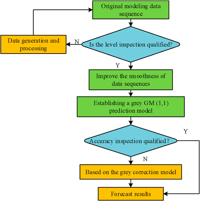
Figure 2. Initial value correction process.

In Figure 2, the initial value corrected grey prediction GM(1,1) model first performs a rank ratio test on the initial sequence, and sequences that fail the test need to undergo data cleaning and function transformation preprocessing; Subsequently, a GM(1,1) model is built and its accuracy is verified. For prediction results with large residuals, initial value correction is introduced to improve the grey model for residual correction. Finally, the optimal prediction model is selected through comparison and applied to engineering practice. This process significantly improves the adaptability and prediction accuracy of traditional grey models to complex data through a progressive optimization strategy of “inspection-transformation-modeling-correction”. The research adopted an initial value correction method based on numerical optimization. The core idea is: to transform the determination of initial conditions from a simple “assignment” to “optimization”, and by minimizing the error between the simulated sequence of the model and the real accumulated sequence, to inversely deduce the theoretical optimal initial value. The initial value correction grey model formula is discretized as shown in Equation 6.

${\mathrm{X}}^{\left(1\right)}\left(K+1\right)=-\frac{\mathrm{C}}{\mathrm{a}}{\mathrm{e}}^{-\mathrm{a}k}+\frac{\mathrm{u}}{\mathrm{a}}(6)$

In Equation 6, ${\mathrm{X}}^{\left(1\right)}\left(K+1\right)$ represents the PV at $\left(K+1\right)$; $C$ represents the integral constant; ${\mathrm{e}}^{-\mathrm{a}k}$ stands for index term. To solve the constant $C$, in the GM(1,1) prediction model, the initial PVs of the accumulated generated sequence remain consistent, as shown in Equation 7.

${\widehat{\mathrm{X}}}^{\left(1\right)}\left(1\right)=-\frac{\mathrm{C}}{\mathrm{a}}+\frac{\mathrm{u}}{\mathrm{a}}={\mathrm{X}}^{\left(0\right)}\left(1\right),-\frac{\mathrm{C}}{\mathrm{a}}={\mathrm{X}}^{\left(0\right)}\left(1\right)-\frac{\mathrm{u}}{\mathrm{a}}(7)$

The determination of initial PVs should be combined with specific application scenarios, and parameters that meet specific conditions should be selected from the range of one to n. The merging process is shown in Equation 8.

$\begin{array}{c}{\mathrm{X}}^{\left(1\right)}\left(K+1\right)=\left({\mathrm{X}}^{\left(1\right)}\left(\mathrm{m}\right)-\frac{\mathrm{u}}{\mathrm{a}}\right){\mathrm{e}}^{-\mathrm{a}k+\mathrm{a}\left(\mathrm{m}-1\right)}+\frac{\mathrm{u}}{\mathrm{a}}\\ =\left({\mathrm{X}}^{\left(1\right)}\left(\mathrm{m}\right)-\frac{\mathrm{u}}{\mathrm{a}}\right){\mathrm{e}}^{-\mathrm{a}\left(k-\mathrm{m}+1\right)}+\frac{\mathrm{u}}{\mathrm{a}}\end{array}(8)$

In Equation 8, $m$ represents the new starting time index; ${\mathrm{e}}^{-\mathrm{a}\left(k-\mathrm{m}+1\right)}$ represents the exponential trend of the accumulated sequence. Therefore, by introducing an initial value correction mechanism, this process effectively solves the prediction bias problem caused by theoretical assumption defects in the traditional GM(1,1) model.

3.2 RBF NN residual correction

The constructed initial value correction GM(1,1) model can address the issue of prediction bias, but its ability to fit non-linear and highly volatile data is poor. RBF NN is a nonlinear function approximator that can fit any complex nonlinear data through Gaussian RBFs (Simani et al., 2024). To compensate for the overfitting problem of the enhanced GM(1,1) model, the study combined RBF NN to solve it. The structure of RBF NN is denoted in Figure 3.

Figure 3

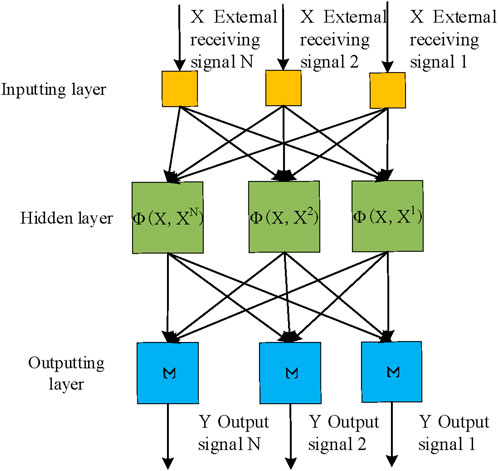
Figure 3. Structure of RBF NN.

In Figure 3, the RBF NN adopts a three-layer topology structure, including an inputting layer, a hidden layer, and an outputting layer. The inputting layer is responsible for receiving external signals $x_1$, $x_2$,., $x_n$ and performing preliminary transmission. The hidden layer implements nonlinear transformation through RBFs to map input features to a high-dimensional feature space. The outputting layer nodes obtain the output signal of the hidden layer, which is then weighted and summed to generate the final outputs $y_1$, $y_2$, $y_n$. The signal is then transmitted back and received by the inputting layer. The hidden layer performs nonlinear response, and the outputting layer linearly fuses the results to extract features using RBFs of local responses. The outputting layer linearly simplifies training, balancing nonlinear fitting and training efficiency. It is broadly utilized in scenarios such as function approximation and pattern recognition. The input data of the RBF NN is standardized, as denoted in Equation 9.

${\widehat{\mathrm{X}}}_i\left(k\right)=\frac{{\mathrm{X}}_i\left(k\right)-{\overline{\mathrm{X}}}_i}{{\mathrm{\delta }}_i}(9)$

In Equation 9, ${\widehat{\mathrm{X}}}_i\left(k\right)$ means the normalized value of the $i$ th variable and the $k$ th sample; ${\overline{\mathrm{X}}}_i$ stands for mean; ${\mathrm{\delta }}_i$ stands for standard deviation. The output results need to be restored to obtain the actual values, as shown in Equation 10.

${\mathbf{y}}_i={\overline{\mathbf{y}}}_i+{\mathrm{\delta }}_i{\widehat{\mathbf{y}}}_i(10)$

In Equation 10, ${\mathbf{y}}_i$ represents raw scale data; ${\overline{\mathbf{y}}}_i$ represents the standardized mean; ${\widehat{\mathbf{y}}}_i$ represents standardized data. To ensure that the networked control system does not transform into an open-loop system, an RBF networked predictive control system scheme is added here. The process is shown in Figure 4.

Figure 4

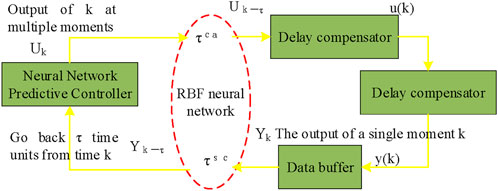
Figure 4. RBF network predictive control system.

As shown in Figure 4, the predictive control system based on RBF NN adopts a time-driven mechanism, which is composed of three core modules working together: the data buffer is responsible for storing and managing time-series data, the NN predictive controller realizes intelligent decision-making, and the delay compensator handles network transmission delay problems. The system adopts a synchronous clock mechanism, and all sensors, controllers, and actuators maintain strict time synchronization. To ensure the reliability of data transmission, each data packet is marked with an accurate timestamp indicating the time of transmission. To address the potential issues of out of order and packet loss in network transmission, the system encapsulates cached output data with corresponding timestamps into data packets to ensure data integrity and timing. The solution is shown in Equation 10.

$Y_k=\left\{y\left(k\right),y\left(k-1\right),\dots ,y\left(k-{\overline{\tau }}^{sc}\right),k\right\}(11)$

In Equation 11, $y$ represents the output at a single moment; ${\overline{\tau }}^{sc}$ represents the lag parameter. Due to the impact of network latency, the system output data obtained by the controller at $t$ time is not real-time data, but a historical data sequence with delay, as shown in Equation 12.

$Y_{k-{\tau }_k^{\infty }}=\left\{y\left(k-{\tau }_k^{sc}\right),y\left(k-1-{\tau }_k^{sc}\right),\dots ,y\left(k-{\overline{\tau }}^{sc}-{\tau }_k^{sc}\right),k-{\tau }_k^{sc}\right\}(12)$

In Equation 12, $Y_{k-{\tau }_k^{\infty }}$ represents the historical data set strongly correlated with time $k-{\tau }_k^{sc}$; $k-{\tau }_k^{sc}$ stands for time marker; ${\tau }_k^{sc}$ represents the lag associated with time $k$. The core innovation of the research in methodology is reflected in the dual optimization framework of “theory-driven and data-driven”. Firstly, for the GM(1,1) model, the study abandoned the traditional assumption of taking the initial value x(1) (1) as a deterministic condition and reconstructed it into an optimizable integral constant C. The systematic bias was theoretically eliminated by establishing an optimization problem aimed at minimizing the sum of squares of the residuals between the simulated sequence and the real cumulative sequence and deriving its analysis. Secondly, for the fusion strategy, the study adopted a dynamic weighting algorithm based on the variance of prediction errors. The significance of this strategy lies in its mathematical optimality, which ensures that the overall variance of prediction errors after fusion is minimized. These two improvements not only make the model have a more solid theoretical foundation, but also its superior performance can be explained by strict mathematical criteria. The study integrates RBF NNs and designs an RBF networked predictive control system with integrated timestamp synchronization and data caching, which can significantly enhance the efficacy of the initial value modified GM(1,1) model for nonlinear data fitting, while alleviating the latency and disorder problems in network transmission.

3.3 Construction of hybrid prediction model

Considering the characteristics of robot fault prediction tasks involving both trend changes and complex nonlinear features, a single prediction model often struggles to fully capture data characteristics. The hybrid modeling method combines the advantages of different models to simultaneously handle deterministic trends and stochastic fluctuations in data, thereby significantly improving predictive performance. The study constructs a robot fault prediction framework based on the improved GM(1,1) model and RBF by integrating the initial value modified improved gray model GM(1,1) with RBF NN for feature extraction and its predictive control scheme. The framework structure is shown in Figure 5.

Figure 5

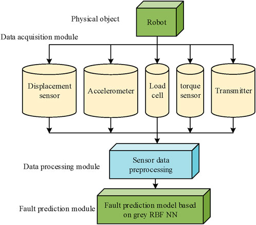
Figure 5. Fault prediction framework of grey RBF robot.

As shown in Figure 5, the core architecture of the predictive maintenance system starts from the underlying physical object - the robot, and monitors its key physical states (such as position, vibration, force, torque) in real time through various sensors (including displacement sensors, accelerometers, load sensors, torque sensors) in the data acquisition module. After the sensor data is transmitted through the transmitter, it enters the data processing module for necessary sensor data preprocessing (such as cleaning, filtering, feature extraction) to convert it into high-quality and suitable feature data for analysis. Finally, the processed data are fed into the top-level fault prediction module, which uses a fault prediction model based on grey theory and RBF NN for intelligent analysis. The aim of this is to predict potential faults that may occur in the robot in advance and achieve active maintenance. The entire process clearly outlines the complete chain from physical signal perception, data transmission and processing to intelligent prediction. By reasonably determining the weight coefficient vector, a combined prediction model is built, as denoted in Equation 13.

$P_{\mathrm{c}}={\lambda }_1{P}_1+{\lambda }_2{P}_2(13)$

In Equation 13, $P_{\mathrm{c}}$ represents the final result after weighted fusion; ${\lambda }_1$ and ${\lambda }_2$ represent weight coefficients; $P_1$ and $P_2$ represent weighted base quantities. Research has shown that the core mechanism of this combination model is reflected in the linear combination process of weight coefficients. The research focuses on the improvement of the GM(1,1) model and the dynamic weighted fusion algorithm based on error variance for RBF. This algorithm determines the optimal weight allocation by quantifying the stability of the prediction results of each sub-model, as shown in Equation 14.

$\begin{array}{c}{\mathrm{\sigma }}_{gm}^2=\text{Var}\left({\mathrm{E}}_{gm}\right)\\ {\mathrm{\sigma }}_{rbf}^2=\text{Var}\left({\mathrm{E}}_{rbf}\right)\end{array}(14)$

In Equation 14, ${\mathrm{\sigma }}_{gm}^2$ represents the variance of the random variable $GM$ related to $E_{gm}$. ${\sigma }_{rbf}^2$ represents the variance of the random variable $MF$ related to $E_{rbf}$; $\text{Var}$ represents variance. From this, the final prediction can be obtained, as shown in Equation 15.

$P_{final}={\lambda }_{gm}·P_{gm}+{\lambda }_{rbf}·P_{rbf}(15)$

In Equation 15, $P_{final}$ represents the final fusion result; “ ${\lambda }_{gm}$” represents the weight coefficient of $GM$. $P_{gm}$ indicates the prediction result; “ ${\lambda }_{rbf}$” represents the weight coefficient of $MF$. Therefore, a new combination prediction system was constructed by organically integrating the grey prediction model with the RBF NN model. Figure 6 showcases the complete workflow of the grey RBF NN hybrid model.

Figure 6

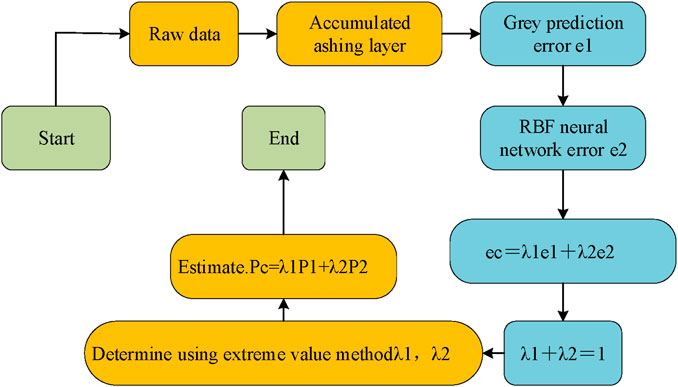
Figure 6. Process of the combined prediction model of grey RBF NN.

The amalgamation of the grey prediction model and the RBF NN model to form a combined prediction process is illustrated in Figure 6. The process begins with the input of raw data, which is simultaneously fed into the grey prediction model and RBF NN model for parallel prediction, and their respective prediction error values $e1$ and $e2$ are calculated. Subsequently, the system uses the extremum method to determine the optimal weight coefficients $\lambda 1$ and $\lambda 2$ for the two models, which must satisfy the constraint condition $\lambda 1+\lambda 2=1$ (and usually non-negative). The final result $Pc$ of the combined prediction is calculated using formula $Pc=\lambda 1P1+\lambda 2P2$, which is the weighted average of the PVs $P1$ (grey model) and $P2$ (RBF model) of two independent models. The total error $ec$ of the combined prediction is calculated according to formula $ec=\lambda 1e1+\lambda 2e2$. The goal of the whole process is to minimize the combination error $ec$ by dynamically optimizing the weight, so as to generate a more accurate and robust prediction result $Pc$ than a single model. A hybrid model for robot fault prediction combining improved GM(1,1) grey model and RBF NN has been proposed, which solves the theoretical shortcomings of traditional grey prediction through initial value correction and enhances the non-linear data fitting ability using NN. The system adopts the extreme value method to dynamically optimize the model weight $\lambda 1+\lambda 2=1$, generates the prediction result $Pc=\lambda 1P1+\lambda 2P2$ through weighted fusion, and minimizes the combination error $ec=\lambda 1e1+\lambda 2e2$.

4 Validation of robot fault prediction model based on improved GM(1,1) model and RBF

4.1 Performance verification of improved GM(1,1) model

To evaluate the performance of a robot fault prediction model based on the improved GM(1,1) model and RBF, this study compared it with the unimproved GM(1,1) prediction model and RBF prediction model. The core objective of the experiment was to verify the performance of the proposed model in predicting the key state parameters of the robot, thereby providing a basis for FD. The experimental subject was the second joint of the Ruiman RM65 industrial robot. The study chose the current of the joint motor as the prediction target variable because it can sensitively reflect the increased load torque changes due to mechanical wear and is a precursor indicator for fault prediction. Data was collected through a high-precision current sensor with a sampling frequency of 10 kHz and then downsampled to 1 kHz for analysis. All the PVs and errors in the study refer to the predictions of motor current. The health status of mechanical components was inferred by analyzing the trend of the current prediction sequence, and the remaining useful life was calculated accordingly. Ultimately, the output of the model was the fault probability or RUL estimate, which was based on the high-precision and multi-step prediction capability of the current signal. The research data was derived from the industrial robot fault simulation and operation datasets of the PYY and LJP laboratories. Multi-source sensors such as accelerometers, encoders, and temperature sensors were used to collect vibration, motion, load, and temperature signals at a sampling frequency of 25.6 kHz. By extracting 42 time-domain and frequency-domain features such as root mean square, kurtosis and centroid frequency from the original signal, the remaining useful life was taken as the prediction target. The dataset contains 18 full life cycle data records under five failure modes. The training set (12 records) and the test set (6 records) were divided according to the records, and Z-score standardization processing was carried out. The parameters of the experimental equipment are detailed in Table 1.

Table 1

Table 1. Experimental equipment parameter table.

The study selected the Ruiman RM65 series robot, which is a lightweight robotic arm with a fiberglass shell. Its total structural length is approximately 850.5 mm and it has a compact spherical workspace. The schematic diagram illustrating its structural configuration is presented in Figure 7.

Figure 7

Figure 7. Rylerman RM65 robot.

According to the above model parameters, this study evaluated the fault prediction performance of the model by comparing the error prediction of the GM(1,1) model before and after improvement, comparing the RBF NN model with the comprehensive model, comparing the true value with the PV, and comparing the model before and after improvement at different speeds. Firstly, a comparison was made between the error prediction of the GM(1,1) model before and after improvement, and the experimental results are shown in Figure 8.

Figure 8

Figure 8. Comparison of error prediction before and after GM(1,1) model modification. (a) Traditional grey model and actual values. (b) Optimize grey model and actual values.

In Figure 8a, the PVs of the classical grey model exhibited a relatively gentle trend of change, with overall fluctuations being relatively small. From Figure 8b, optimizing the grey model’s PVs exhibited a more sensitive adjustment ability, which can closely track changes in actual data, especially with better adaptability near turning points. Overall, the optimized grey model performs better than the classical grey model in prediction accuracy and dynamic response, and its prediction curve is more in line with the fluctuation characteristics of actual data.

4.2 Performance verification of RBF NN and fusion model

On the basis of verifying the predictive performance of the optimized GM(1,1) model, to further validate the practical application value of the model combined with RBF, the study selected LJP laboratory data for experiments and compared the sample error between the RBF prediction model and the combination model, as shown in Figure 9.

Figure 9

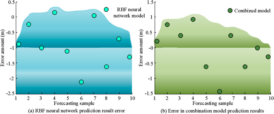
Figure 9. Comparison between RBF prediction model and fusion model. (a) RBF neural network prediction result error. (b) Error in combination model prediction results.

As shown in Figure 9a, from the blue error value area, the error range span was relatively large. Among them, the error distribution of the blue spherical RBF NN showed obvious volatility, such as the appearance of discrete values like −2.5 and 0.5, indicating that there is a significant deviation in the prediction of some samples by this model. In Figure 9b, the overall error value of the combined model was closer to the zero baseline, and the variation amplitude was relatively gentle. Overall, the combined model prediction results are not only more accurate, but also have better stability. Afterwards, to prove the actual prediction accuracy of the combined model, the PVs were compared with the true values, and the findings are denoted in Figure 10.

Figure 10

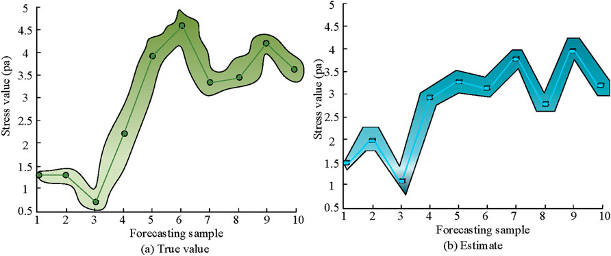
Figure 10. Comparison of PV and true value. (a) True value. (b) Estimate.

In Figure 10a, the actual observed value distribution of the target variable is presented. From the perspective of data distribution, the true values exhibited obvious nonlinear characteristics, with dense data points in the middle range (approximately 2–4.5 units) and relatively sparse data points at both ends. In Figure 10b, the model’s PVs generally followed the trend of the true values well, especially in the data intensive middle region (2–4.5 units), where the predicted curve almost overlapped with the true value curve. The research findings denote that the combination prediction model has high prediction accuracy for conventional data. Finally, to prove the prediction speed and prediction error of the combined model, the study compared its prediction error rate with that of the traditional model, and the results are shown in Figure 11.

Figure 11

Figure 11. Comparison of speed error between traditional model and combination model. (a) 0.1m/s. (b) 0.4m/s.

In Figure 11a, the prediction error of the traditional model fluctuated in the range of 0.5–0.7 m/s, with the maximum error occurring at the third and fifth sample points (0.44 m/s), exhibiting periodic fluctuations. The combination model significantly narrowed the error range (0.55–0.62 m/s) and reduced the overall mean error by about 40%. As shown in Figure 11b, the traditional model showed a persistently high prediction (0.05 m/s) under high-speed conditions (Y = 0.4 m/s). The combined model corrected the system deviation, and the correlation coefficient between the PV and the true value remained basically unchanged. The error curve became flatter and the standard deviation decreased. The above results indicate that the combination model achieves significant results in error control, stability improvement, and system deviation correction through algorithm optimization, providing a more reliable technical solution for the engineering application of fault prediction systems.To enhance the rigor and persuasiveness of the research, comparative experiments with mainstream prediction methods were introduced. In this experiment, on the same dataset, the exact same training set/test set partitioning was adopted to compare the performance of the improved GM(1,1)-RBF hybrid model proposed in the study with that of the classical time series prediction method - the autoregressive integral moving average model. The evaluation comprehensively considered the prediction accuracy and used mean absolute error (MAE), root mean squared error (RMSE) and mean absolute percentage error (MAPE|) as the core evaluation indicators. Meanwhile, the study conducted an in-depth analysis of the independent contributions of each improved component proposed by the research through ablation experiments. All results were reported with 95% confidence intervals and statistical significance relative to the GM(1,1) baseline was calculated through paired tests. The comparison results are shown in Table 2.

Table 2

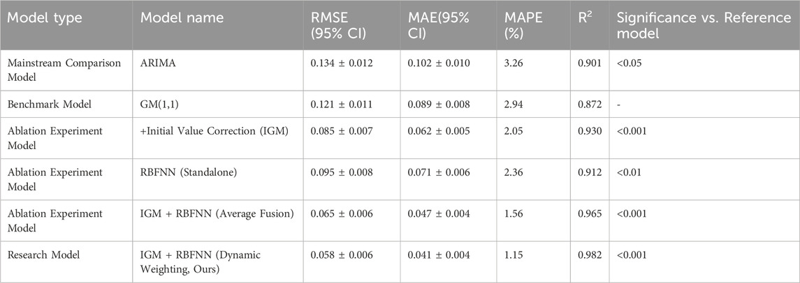
Table 2. Comprehensive performance comparison and ablation experiment analysis.

The results showed that the proposed IGM-RBF dynamic weighted fusion model was significantly superior to the comparison methods in terms of prediction accuracy. Its RMSE was reduced to 0.058, which was 56.7% and 52.1% higher than that of the ARIMA model and the traditional GM(1,1) benchmark, respectively. The ablation experiment further verified the effectiveness of each innovative component: the initial value correction mechanism alone contributed a 29.8% performance improvement, while the dynamic weighted fusion strategy ultimately achieved a significantly better effect than the simple average fusion. All improvements passed the 95% confidence interval and statistical significance test (p < 0.001), fully demonstrating the accuracy and reliability of the hybrid model in the fault prediction of industrial robots.

5 Conclusion

A hybrid prediction method combining initial value correction GM(1,1) model and RBF NN was proposed to address the theoretical deficiencies and insufficient nonlinear fitting of traditional GM(1,1) model in robot fault prediction. By introducing an initial value correction mechanism to enhance the GM(1,1) model and combining it with an RBF NN to construct a hybrid prediction model, the extreme value method was utilized to dynamically optimize the weight coefficients, ultimately forming a complete framework for robot fault prediction. By combining the theory-driven initial value optimization algorithm with the data-driven nonlinear correction, the problems of initial sensitivity and insufficient nonlinear fitting of the traditional grey model in robot fault prediction were fundamentally solved.The experimental results showed that the improved GM(1,1) model achieved a 40% improvement in prediction accuracy compared to traditional models. This improvement was particularly prominent in terms of response speed at turning points, indicating a significant enhancement in the model’s ability to handle sudden changes. The combination model further optimized the prediction performance, effectively reducing the error range from 0.2–1.0 m/s to 0–0.6 m/s. At the same time, the overall mean error was reduced by 40%, and the standard deviation was also reduced by 62%. This means that the stability and accuracy of the prediction results have been greatly improved. Under high-speed conditions, when the speed reached 0.4 m per second, the correlation coefficient increased from 0.82 to 0.95, effectively correcting the system deviation and significantly improving the overall reliability and practicality of the model. Overall, the proposed hybrid prediction model significantly improves the accuracy, stability, and adaptability of fault prediction through algorithm fusion and structural optimization. Although the research model has shown excellent performance and application effects, there are still some limitations in the research. Currently, the prediction effect under a single fault mode has been mainly verified, but its applicability in multi-fault coupling scenarios still needs to be verified. The optimization of hyperparameters still requires manual intervention. The long-term stability in real industrial environments needs further verification. In the future, it will consider the prediction performance under multiple fault coupling scenarios, and further research can explore these limitations in depth.

Data availability statement

The original contributions presented in the study are included in the article/supplementary material, further inquiries can be directed to the corresponding author.

Author contributions

LC: Writing – original draft, Writing – review and editing.

Funding

The author(s) declare that no financial support was received for the research and/or publication of this article.

Conflict of interest

The author declares that the research was conducted in the absence of any commercial or financial relationships that could be construed as a potential conflict of interest.

Generative AI statement

The author(s) declare that no Generative AI was used in the creation of this manuscript.

Any alternative text (alt text) provided alongside figures in this article has been generated by Frontiers with the support of artificial intelligence and reasonable efforts have been made to ensure accuracy, including review by the authors wherever possible. If you identify any issues, please contact us.

Publisher’s note

All claims expressed in this article are solely those of the authors and do not necessarily represent those of their affiliated organizations, or those of the publisher, the editors and the reviewers. Any product that may be evaluated in this article, or claim that may be made by its manufacturer, is not guaranteed or endorsed by the publisher.

References

Ballou, A., Alameda-Pineda, X., and Reinke, C. (2023). Variational Meta reinforcement learning for social robotics. Appl. Intell. 53 (22), 27249–27268. doi:10.1007/s10489-023-04691-5

CrossRef Full Text | Google Scholar

Damak, K., Boujelbene, M., Acun, C., Alvanpour, A., Das, S. K., Popa, D. O., et al. (2025). Robot failure mode prediction with deep learning sequence models. Neural Comput. Appl. 37 (6), 4291–4302. doi:10.1007/s00521-024-10856-1

CrossRef Full Text | Google Scholar

D’Amico, G., De Blasis, R., and Vigna, V. (2025). Energy production forecasting: an application of the grey markov chain model to data from Italy. Renew. Sustain. Energy 3 (1), 1–23. doi:10.55092/rse20250003

CrossRef Full Text | Google Scholar

Islam, M. D. S., Kim, M. J., Ku, K. M., Kim, H. Y., and Kim, K. (2024). Study on fault diagnosis and data processing techniques for substrate transfer robots using vibration sensor data. J. Microelectron. Packag. Soc. 31 (2), 45–53. doi:10.3182/20110828-6-IT-1002.02842

CrossRef Full Text | Google Scholar

Li X, X., Guo, J., Qiao, Z., and Zhao, F. (2025). Air quality prediction based on a new discrete variable weight multivariable grey model. Water Air and Soil Pollut. 236 (7), 473–26. doi:10.1007/s11270-025-08136-2

CrossRef Full Text | Google Scholar

Li, H., Wu, Z., Qian, S., and Duan, H. (2023). A novel fractional-order grey prediction model: a case study of Chinese carbon emissions. Environ. Sci. Pollut. Res. 30 (51), 110377–110394. doi:10.1007/s11356-023-29919-2

PubMed Abstract | CrossRef Full Text | Google Scholar

Li, H., Hu, X., Zhang, X., Chen, H., and Li, Y. (2024a). Adaptive radial basis function neural network sliding mode control of robot manipulator based on improved genetic algorithm. Int. J. Comput. Integr. Manuf. 37 (8), 1025–1039. doi:10.1080/0951192x.2023.2294439

CrossRef Full Text | Google Scholar

Li, Y., Ren, H., and Liu, J. (2024b). A novel fractional multivariate grey prediction model for forecasting hydroelectricity consumption. Grey Syst. Theory Appl. 14 (3), 507–526. doi:10.1108/GS-09-2023-0095

CrossRef Full Text | Google Scholar

Li P, P., Zhou, C., and Du, X. (2025). Evaluation and prediction of surface water pollution in China based on improved entropy-weighted TOPSIS algorithm and metabolism GM (1, 1) grey model. J. Industrial Manag. Optim. 21 (2), 1600–1629. doi:10.3934/jimo.2024140

CrossRef Full Text | Google Scholar

Luo, R., Zhao, S., Kuck, J., Ivanovic, B., Savarese, S., Schmerling, E., et al. (2024). Sample-efficient safety assurances using conformal prediction. Int. J. Robotics Res. 43 (9), 1409–1424. doi:10.1177/02783649231221580

CrossRef Full Text | Google Scholar

Narayan, J., Abbas, M., Patel, B., and Dwivedy, S. K. (2023). Adaptive RBF neural network-computed torque control for a pediatric gait exoskeleton system: an experimental study. Intell. Serv. Robot. 16 (5), 549–564. doi:10.1007/s11370-023-00477-3

CrossRef Full Text | Google Scholar

Nguyen, V. G., Duong, X. Q., Nguyen, L. H., Nguyen, P. Q. P., Priya, J. C., Truong, T. H., et al. (2023). An extensive investigation on leveraging machine learning techniques for high-precision predictive modeling of CO2 emission. Energy Sources, Part A Recovery, Util. Environ. Eff. 45 (3), 9149–9177. doi:10.1080/15567036.2023.2231898

CrossRef Full Text | Google Scholar

Pan, J., Qu, L., and Peng, K. (2023). Research on robotic manipulator fault detection and diagnosis technology based on machine vision in complex environments. J. Field Robotics 40 (2), 231–242. doi:10.1002/rob.22125

CrossRef Full Text | Google Scholar

Peng, B., Gao, D., Wang, M., and Zhang, Y. (2024). 3D-STCNN: Spatiotemporal convolutional neural network based on EEG 3D features for detecting driving fatigue. J. Data Sci. Intelligent Syst. 2 (1), 1–13. doi:10.47852/bonviewJDSIS3202983

CrossRef Full Text | Google Scholar

Rabbani, A., Samui, P., and Kumari, S. (2023). A novel hybrid model of augmented grey wolf optimizer and artificial neural network for predicting shear strength of soil. Model. Earth Syst. Environ. 9 (2), 2327–2347. doi:10.1007/s40808-022-01610-4

CrossRef Full Text | Google Scholar

Simani, S., Lam, Y. P., Farsoni, S., and Castaldi, P. (2024). Dynamic neural network architecture design for predicting remaining useful life of dynamic processes. J. Data Sci. Intelligent Syst. 2 (3), 141–152. doi:10.47852/bonviewJDSIS3202967

CrossRef Full Text | Google Scholar

Song, Z., Shi, H., Bai, X., and Li, G. (2023). Digital twin-assisted fault diagnosis system for robot joints with insufficient data. J. Field Robotics 40 (2), 258–271. doi:10.1002/rob.22127

CrossRef Full Text | Google Scholar

Sun, Y. (2023). Automatic vibration control method for grasping end of flexible joint robot. J. Vibroengineering 25 (8), 1502–1515. doi:10.21595/jve.2023.23264

CrossRef Full Text | Google Scholar

Wang, T., Zhang, L., and Wang, X. (2023). Fault detection for motor drive control system of industrial robots using CNN-LSTM-based observers. CES Trans. Electr. Mach. Syst. 7 (2), 144–152. doi:10.30941/CESTEMS.2023.00014

CrossRef Full Text | Google Scholar

Zhang, L., Ma, X., He, Q., and Li, T. (2025). A novel unbiased multi-variable grey model. Grey Syst. Theory Appl. 15 (2), 209–238. doi:10.1108/GS-07-2024-0090

CrossRef Full Text | Google Scholar