Thermostating strategies and interaction potentials in interfacial water simulations: are they really needed?

Understanding the molecular behavior of water near solid surfaces is critical for advancing simulations in catalysis, energy storage, and nanoscale heat transfer. Here, we reveal how the choice of thermostating strategy and interaction potential fundamentally alters the structural and dynamical properties of interfacial water. Using classical molecular dynamics (MD) simulations of SPC/E water near a Pt (111) surface, we compare four distinct thermal control schemes in combination with two interaction models: the Zhu-Philpott (ZP) potential and a fitted Lennard-Jones (LJ) approximation. Our results demonstrate that thermostating both the water and the solid yields the most realistic layering, orientation, and thermal equilibration in the first hydration layer (∼0.5 nm from the surface). Surprisingly, simulations using only water thermostats but with a frozen or non-thermostated wall produce overstructured or thermally biased interfacial profiles. Furthermore, we show that a carefully optimized LJ potential can approximate ZP’s accuracy in density layering but fails to replicate angular orientation. The study points out the situations where simplified models are valid, and where detailed interactions and thermal effects must be included, offering both new knowledge and useful rules for improving simulation accuracy.

1 Introduction

The behavior of water at solid interfaces is central to a wide range of technological and scientific applications, including catalysis, heat transfer, energy storage, corrosion, and biomedical device design. At the molecular scale, the structure and dynamics of water near solid surfaces are governed by a complex interplay of intermolecular forces, surface chemistry, and thermal fluctuations (Maccarini, 2007; Plawsky et al., 2008; Peng et al., 2022). In particular, the interactions between water molecules and metal surfaces have attracted significant attention due to their relevance in electrochemical and thermal systems. Since the 1940s, the structural characteristics of water at metal interfaces have been the subject of sustained scientific investigation (Henniker, 1949; Drost-Hansen, 1969; Ribarsky et al., 1985). Each decade has brought significant progress in understanding how water molecules organize near solid surfaces. One of the earliest and most influential contributions came from Henniker (1949), who, in a seminal review (Henniker, 1949), compiled both direct and indirect experimental evidence showing that molecular orientation at liquid surfaces can extend far beyond a single molecular layer. He introduced the concept of “deep surface orientation”, in which alignment at the interface propagates into the bulk through successive polarization of neighboring molecules. His work also discusses the ongoing debates within the scientific community on the existence of intermolecular forces longer than a few Angstroms, but shorter than classical physics. In 1969, Drost-Hansen, in his seminal paper (Drost-Hansen, 1969), introduces the three-layer model for water, through which he tried to conceptualize the structure of water to be greatly influenced by the adjacent lattice layers of metal. The review paper (Thiel and Madey, 1987) of Thiel and Madey’s (1987) underscores the complexity and variability of water-surface interactions. The behavior of water is not only surface-specific but also coverage- and temperature-dependent. Their synthesis of experimental findings establishes a baseline for understanding how water behaves in catalytic processes, corrosion, atmospheric chemistry, and biological systems.

From 2000 onward, advancements in both simulation and experimental techniques have significantly deepened our understanding of water structuring and dynamics at metal interfaces. A central development has been the rise of ab initio molecular dynamics (AIMD) simulations, which use quantum mechanical descriptions (typically density functional theory) to model electronic interactions between water molecules and metal surfaces. AIMD studies have revealed fine-grained details such as charge transfer effects, hydrogen bond rearrangements, and specific adsorption geometries that were previously inaccessible with classical models. For instance, studies on water adsorption on Pt (111), Au (111), and Ru (0001) surfaces using AIMD have demonstrated that the orientation and binding energy of interfacial water molecules are highly sensitive to the local electronic structure of the substrate, as well as temperature and water coverage (Michaelides, 2003; Carrasco et al., 2012; Natarajan and Behler, 2016; Le et al., 2021; Groß and Sakong, 2022a).

However, the high computational cost of AIMD restricts its applicability to relatively small systems (typically <100 atoms) and short simulation timescales (a few tens of picoseconds) (Iftimie et al., 2005; He et al., 2018; Jia et al., 2020; Joll et al., 2024). As a result, the development of improved classical potentials that retain some of the electronic fidelity of AIMD, but at a fraction of the cost, has been a key focus. One notable advancement in this area is the Zhu–Philpott (ZP) potential (Zhu and Philpott, 1994; Zhu, 1995), a classical potential specifically designed to simulate water–metal interactions more accurately than the traditional Lennard-Jones (LJ) framework. ZP potential decomposes the interaction into three physically motivated components: (1) a conduction electron image charge interaction that mimics the polarization effects induced by the metal, (2) an anisotropic attraction capturing directional bonding preferences of water molecules, and (3) an isotropic repulsive component accounting for Pauli exclusion. This framework provides a more realistic representation of the energy landscape experienced by water molecules at a metallic interface and has shown good agreement with AIMD results in terms of hydration structure and dipole orientation near platinum surfaces (Zhu and Philpott, 1994; Chen et al., 2018; Li et al., 2021).

Although not yet widespread due to implementation complexity, recent studies have begun to incorporate the ZP potential into large-scale MD simulations, confirming its ability to reproduce experimental observations such as layering in oxygen density profiles and preferred dipole orientations (Kimura and Maruyama, 2002; Shi and Dhir, 2009; Steinmann et al., 2018). ZP potential serves as a critical bridge between AIMD accuracy and classical MD scalability, making it a valuable tool for interfacial modeling.

On the experimental front, the last 2 decades have also seen substantial advances in surface-sensitive characterization techniques. X-ray reflectivity (XRR), sum-frequency generation (SFG) spectroscopy, and scanning tunneling microscopy (STM) have all contributed to revealing the layered structure of water at metal surfaces. For instance, SFG studies have directly observed the orientation and hydrogen bonding states of interfacial water, confirming theoretical predictions of surface-aligned dipole vectors. XRR experiments have quantitatively measured the spacing and intensity of water density peaks near metal interfaces, validating the concept of hydration layering up to 2–3 molecular diameters (Fenter and Lee, 2014; Guo et al., 2018; Sanders and Petersen, 2019).

Experimental studies and ab initio molecular dynamics (AIMD) simulations have shown that water molecules near metallic surfaces form well-defined hydration layers with distinct structuring and energetics. While classical molecular dynamics (MD) has emerged as a powerful and computationally efficient tool for probing such interfacial behavior (Stauber et al., 2015; Zhang et al., 2016), its fidelity critically depends on the choice of interaction potentials and thermal control strategies. Traditional Lennard-Jones (LJ) based models, though widely used, often fail to capture the image-charge effects and anisotropic interactions that govern water–metal coupling. In contrast, the Zhu-Philpott (ZP) potential incorporates these effects explicitly, providing a more realistic description of interfacial phenomena. However, the high computational cost of ZP has limited its widespread adoption, and a systematic framework for deciding when simpler models are sufficient has not yet been established.

A second but equally important factor in interfacial MD simulations is the thermostating strategy, the way temperature is regulated in the fluid and solid domains. While thermostats are routinely applied to maintain equilibrium, their placement (on water, the substrate, or both) can strongly influence structural and dynamic outcomes. For instance, freezing the solid wall atoms (Yong and Zhang, 2013; Qian et al., 2016; Skarbalius et al., 2021) improves computational efficiency but artificially suppresses vibrational modes, while failing to thermostat the water near a hot or cold surface can induce nonphysical heating or cooling. Despite its importance, the impact of thermostating on interfacial water structuring has received limited systematic attention.

This study addresses these two critical gaps by (i) establishing a direct connection between LJ and ZP potentials for water–platinum interfaces, and (ii) systematically evaluating how different thermostating strategies influence interfacial water structure and energetics. Using classical MD simulations of SPC/E water on a platinum (111) surface, we implement and validate the ZP potential alongside equivalent LJ parameterizations matched to either energy profiles or density distributions. Four distinct thermostat configurations applied selectively to water, platinum, or both—are then compared to isolate the role of thermal control on properties such as molecular orientation, density layering, radial distribution functions, and interfacial interaction energies.

By bridging simplified and physically detailed interaction models, and by quantifying the consequences of thermostating strategies, our work provides actionable guidelines for achieving simulation fidelity at solid–liquid interfaces. Beyond molecular-level insights, these results establish a foundation for multiscale modeling efforts, including continuum approaches to heat transfer, adsorption, and electrochemical activity at metal–water boundaries. In doing so, this study highlights not only when simplified approximations are valid, but also when explicit treatment of wall dynamics and advanced potentials is essential—offering new pathways for accurate and efficient interfacial simulations.

2 Methods

To investigate the influence of thermostating on systems involving wall-liquid interactions, we consider a model system comprising a three-layer platinum slab with a liquid water slab placed on top of it as shown in Figure 1a. The water molecules are modeled using SPC/E model (Berendsen et al., 1987) and the platinum is modeled as FCC 111 with a lattice constant of $3.924\mathrm{\AA }$ (Arblaster, 1997). The interaction between water molecules is modeled using the standard Lennard-Jones (LJ) potential between oxygen atoms and Coulomb potential between all. The LJ parameters are ${\sigma }_{O-O}=0.316555789nm$ and ${ϵ}_{O-O}=0.155291kcal/mol$ . For the Coulomb potential calculations, the partial charges for hydrogens are $0.4238e$ and that of oxygen is $-0.8476e$.

Figure 1

Figure 1. Molecular configuration used in the MD simulations. Panel (a) displays the side view of the equilibrated system, highlighting the stratification of water molecules near the surface. Panel (b) presents a top-down view, illustrating the formation of a dense interfacial layer. It also shows the orientation of the cartesian coordinate axes and the definition of azimuthal angle $\varphi$. Panel (c) shows the dimensions of the simulation box for spatial reference, with boundary conditions as periodic boundary condition (PBC) along sideways and non-periodic boundary conditions along vertical dimension (z-axis).

A cutoff distance of 3.5σ (∼1.11 nm) was applied for short-range interactions, which requires lateral box dimensions of at least 3.92 nm to avoid periodic artifacts. The vertical (z) dimension was set to 10 nm to leave enough empty space above the water slab, allowing coexistence of liquid and vapor phases and preventing artificial interactions between periodic images. The system contained 2,197 SPC/E water molecules, corresponding to a bulk density of ∼1.0 g/cm³ at 300 K. Similar system sizes (on the order of 1,000–2,000 water molecules) have been widely used in prior interfacial MD studies and shown to provide reliable density layering, orientation distributions, and thermodynamic averages at metal–water interface (Gereben and Pusztai, 2011; Sakamaki et al., 2011a; 2011b; Zhu, 2013; Zhang et al., 2019; Groß and Sakong, 2022b; Zheng et al., 2024). This confirms that our chosen setup is large enough to capture both interfacial structuring near the platinum wall and bulk-like behavior farther away. The complete simulation box is shown in Figure 1c, while Figure 1b highlights the first equilibrated water layer above the platinum surface.

All molecular dynamics (MD) simulations in this study were performed using the LAMMPS simulation package (version: 17 Apr 2024 - Development) (Thompson et al., 2022). Visualization and structural analysis of simulation trajectories were carried out using OVITO (Stukowski, 2009) and VMD (Humphrey et al., 1996). Post-processing and data analysis were conducted using a suite of custom-developed C++ scripts. Initial system construction and preprocessing were performed using Atomsk (Hirel, 2015) in combination with in-house MATLAB codes. Unless explicitly mentioned, below are the parameters used in the study for MD simulations. Time step of integration as $1fs$, equilibration time of $0.5ns$, production time of $0.5ns$. The equations of motion used in this study are based on the formulation by Shinoda et al. (Shinoda et al., 2004), which integrates the hydrostatic pressure control method of Martyna, Tobias, and Klein (Martyna et al., 1994) with the strain energy framework introduced by Parrinello and Rahman (Parrinello and Rahman, 1981). The cutoff radius is 1.2 nm. Since the system that we study is not periodic in all directions, long range Coulomb forces are not estimated using Ewald summation or similar techniques, instead a truncated potential is used. Time integration is carried out using time-reversible and measure-preserving, following the Verlet and rRESPA algorithms developed by Tuckerman et al. (2006).

The simulations used a time step of 1 femtosecond, with an equilibration period of 0.5 ns (500,000 steps) followed by a production run of 0.5 ns (500,000 steps). During equilibration, atomic velocities were initialized at 300 K using a Gaussian distribution, and a Nosé–Hoover thermostat (Hoover, 1985; Nosé, 2002) was applied separately to the water and platinum atoms. Temperature damping parameters were chosen to ensure smooth thermalization. Additionally, a weak spring force was applied to platinum atoms to maintain structural integrity while allowing vibrational motion.

Thermodynamic outputs were computed every 100 steps, including system temperature, kinetic and potential energy, and the interaction energy between water and platinum. Water orientation distributions were evaluated by constructing geometric vectors from the oxygen to the midpoint between the hydrogen atoms. These vectors were projected into spherical coordinates and accumulated over time to produce both 2D angular density maps and marginal polar plots. To ensure spatial resolution, the simulation box was divided into vertical slices along the z-axis. RDFs were computed in two regions: near the metal–water interface and farther into the bulk. A 1D temperature profile was also obtained along the z-axis using chunk-based averaging. Finally, all simulations were performed under fixed boundary conditions in the z-direction, and periodic conditions in x and y directions.

2.1 Water–Water interactions

The SPC/E interactions are calculated as mentioned in the above section, using LJ potential (Equation 1) and Coulomb potential (Equation 2). The equations used are:

$E_{LJ-WW}=4{ϵ}_{ww}\left[{\left(\frac{{\sigma }_{ww}}{r_{ij}}\right)}^{12}-{\left(\frac{{\sigma }_{ww}}{r_{ij}}\right)}^6\right](1)$

$E_{Coul}=\frac{1}{4\pi {ϵ}_0}\frac{q_i{q}_j}{r_{ij}}(2)$

Here, subscripts $i$ and $j$ are reference to the $i^{th}$ and $j^{th}$ particles (atoms), w means water atoms (only oxygen for SPC/E). $\sigma$ and $ϵ$ are the LJ parameters for the Oxygen-Oxygen interactions. $r_{ij}$ is the distance between $i^{th}$ and $j^{th}$ particles, ${ϵ}_0$ is the permittivity in vacuum.

2.2 Platinum–Platinum interactions

In this study, two approaches are used to model the behavior of platinum atoms at the substrate: (1) as a thermal wall, where the atoms are thermostated and allowed to interact dynamically, and (2) as a frozen wall, where the atoms remain fixed and are excluded from time integration. In the thermal wall configuration, a Nosé–Hoover thermostat is applied to maintain the desired temperature, and interatomic forces among platinum atoms are described using the Modified Embedded Atom Method (MEAM) potential, with parameters sourced from established literature (Lee et al., 2003). In contrast, the frozen wall configuration assumes static platinum atoms with no internal dynamics or interatomic interactions. Both configurations are employed and systematically compared throughout the study, as discussed in the Results and Discussion section.

2.3 Water–Platinum interactions

Interactions between water and platinum surfaces have been modeled using various approaches in literature. Most existing studies focus on macroscopic interfacial properties such as contact angle and adhesion energy, where standard Lennard-Jones (LJ) potentials are often sufficient. However, a subset of studies has aimed to investigate the microscopic structural orientation of water molecules at metal interfaces using ab initio molecular dynamics (AIMD). While AIMD offers high accuracy, it is computationally intensive and typically restricted to small systems containing fewer than 50 water molecules.

As an alternative, classical potentials such as the Zhu–Philpott (ZP) potential have been developed to capture many of the structural and orientational characteristics of interfacial water observed in AIMD studies, while remaining computationally efficient. Despite its improved accuracy over standard LJ potential, the ZP potential has seen limited adoption, likely due to the complexity of its implementation and its current restriction to flat surfaces. The main equations corresponding to the ZP potential are listed below. Molecular conduction electron potential is given by Equation 3, where the subscripts are $l$ and $k$ to refer to the image charge interactions.

$E_{cond}={\displaystyle \sum _{l,k}}\frac{q_l{q}_k}{2r_{lk}}(3)$

The anisotropic component of the potential is given by Equation 4,

$E_{anis}=4{ϵ}_{p-Pt}{\displaystyle \sum _j}\left[{\left(\frac{{\sigma }_{p-Pt}^2}{{\left(\alpha {\rho }_{pj}\right)}^2+z_{pj}^2}\right)}^6-{\left(\frac{{\sigma }_{p-Pt}^2}{{\left({\rho }_{pj}/\alpha \right)}^2+z_{pj}^2}\right)}^3\right](4)$

The isotropic component of the ZP potential is given by Equation 5,

$E_{iso}=-4{ϵ}_{p-Pt}{\displaystyle \sum _j}\frac{c_{p-Pt}{\sigma }_{p-Pt}^{10}}{r_{pj}^{10}}(5)$

Here, $p$ refers to Oxygen and Hydrogen atoms, $\alpha =0.8$, a scaling factor. ${\sigma }_{O-Pt}=0.27nm$, ${\sigma }_{H-Pt}=0.255nm$. ${ϵ}_{O-Pt}=6.44\times {10}^{-21}J$ and ${ϵ}_{H-Pt}=3.91\times {10}^{-21}J$. The constants $c_{O-Pt}$ and $c_{H-Pt}$ are 1.28 and 1.2 respectively.

To enable its use in our study, we implemented a custom pair style within the LAMMPS source code, along with the necessary supporting modules. The implementation was validated by simulating a single water molecule approaching a platinum surface from above and comparing the computed interaction energy profile with the results reported in the original ZP potential study (Zhu and Philpott, 1994; Zhu, 1995), showing excellent agreement.

2.4 Summary of simulation parameters

For clarity and ease of reference, all the key parameters used in this study are consolidated into Table 1. These include the water and platinum models, water–platinum interaction potentials (ZP and equivalent LJ fits), simulation box dimensions, time integration details, and the thermostating schemes investigated. While individual parameters are described in detail in the corresponding subsections above, the table provides a concise overview of the complete setup.

Table 1

Table 1. Simulation parameters used in this study.

Further, to validate the code implementation, we have used the oxygen atom density distribution and molecular orientation of water molecules. The density distribution is estimated based on the following equation and plotted in Figure 2. The mathematical equation used for averaging is shown below in Equation 6.

${\rho }_k=\frac{1}{N_t}\sum _{t=1}^{N_t}\frac{N_k\left(t\right)}{A.\Delta z}(6)$

Figure 2

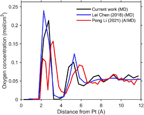
Figure 2. Line graph showing oxygen concentration (mol/cm³) versus distance from Pt (angstroms). Three lines represent different studies: black for current work (MD), blue for Chen et al. (2018), MD, and red for Li et al. (2021), AIMD. Peaks occur between 2 and 4 angstroms, with the concentration generally approaching zero by 12 angstroms.

Here, ${\rho }_k$ is the oxygen number density, $N_k\left(t\right)$ is the number of oxygen atoms in bin $k$ at time $t$. $A$ is the cross-sectional area of the simulation box in x-y plane (parallel to platinum surface). $\Delta z$ is the thickness of each bin, $N_t$ is the total number of time snapshots used during the total sampling time $T$. Each atom’s z-position is extracted from the trajectory file and allocated to the corresponding bin using nearest grid point approach (Hockney and Eastwood, 2021).

Figure 2 presents the oxygen density distribution obtained from our molecular dynamics (MD) simulations using the implemented Zhu–Philpott (ZP) potential. The results are compared with previous MD studies employing the same potential, as well as with ab initio molecular dynamics (AIMD) simulations. The comparison demonstrates agreement between our implementation and the earlier MD results.

While density distribution profiles and radial distribution functions (RDFs) provide valuable insights into the structural arrangement of water near metal surfaces, they offer limited information about molecular orientation. To gain a deeper understanding of the interfacial water structure, we introduce an analysis based on molecular orientation vectors. Specifically, for each water molecule, a vector is defined in a spherical coordinate system centered at the oxygen atom and pointing toward the midpoint between the two hydrogen atoms. This vector, though analogous to a dipole vector, does not strictly follow the electrostatic dipole moment defined by charge distribution, but rather serves as a geometric descriptor of molecular orientation.

A schematic illustration of this construction is provided in Figure 3. The orientation vector is expressed in spherical coordinates, where the polar angle $\theta$ represents the angle with respect to the surface-normal (z-axis), ranging from 0° to 180°, and the azimuthal angle $\varphi$ describes the in-plane rotation around the z-axis, ranging from 0° to 360°. This orientation framework forms the basis for analyzing angular distributions and spatial ordering of water molecules near the platinum interface.

Figure 3

Figure 3. Geometric definition of the water molecule orientation vector. The orientation vector is illustrated relative to the simulation coordinate system, where the z-axis denotes the surface normal of the metal substrate used in the MD simulations.

Based on the orientation vector definition, we visualize the angular distribution of water molecules using two complementary approaches: a 2D orientation density plot and a polar overlay plot. For the 2D density mapping, we define a geometric orientation vector ${\overrightarrow{v}}_i$ for each water molecule iii, constructed from atomic positions as per Equation 7,

${\overrightarrow{v}}_i=\frac{1}{2}\left({\overrightarrow{r}}_{H1}+{\overrightarrow{r}}_{H2}\right)-{\overrightarrow{r}}_O(7)$

where ${\overrightarrow{r}}_O$ is the position of the oxygen atom, and ${\overrightarrow{r}}_{H1},{\overrightarrow{r}}_{H2}$ are the positions of the hydrogen atoms. This vector, although geometric, closely resembles the molecular dipole vector and captures the orientation of the water molecule. The vector ${\overrightarrow{v}}_i$ is converted to spherical coordinates to extract the polar angle ${\theta }_i$ and the azimuthal angle ${\varphi }_i$ Equations 8, 9 respectively.

${\theta }_i=co{s}^{-1}\left(v_z,i\right),{\theta }_i\in \left[0°,180°\right](8)$

$\left.{\varphi }_i=\mathit{atan}2\left(v_{y,i},v_{x,i}\right)\mathit{mod}360°,{\varphi }_i\in [0°,360°\right)(9)$

These angles are then binned into a 2D histogram for each simulation frame $t$, using Equation 10:

$H_t\left({\theta }_j,{\varphi }_k\right)={\displaystyle \sum _{i=1}^{N_t}}\delta {\theta }_j{\theta }_i·\delta {\varphi }_k{\varphi }_i(10)$

where $N_t$ is the number of water molecules in frame $t$, and $\delta$ is the Kronecker delta function indicating whether a molecule’s orientation falls into bin $\left({\theta }_j,{\varphi }_k\right)$. The histograms are then averaged over all $T$ frames using Equation 11:

$\overline{H}\left({\theta }_j,{\varphi }_k\right)=\frac{1}{T}{\displaystyle \sum _{i=1}^T}{H}_t\left({\theta }_j,{\varphi }_k\right)(11)$

Since raw histograms can appear pixelated and may obscure trends in orientation, we apply 2D Gaussian smoothing using a kernel defined as per Equation 12:

$G\left(m,n\right)=\frac{1}{2\pi {\sigma }_{\theta }{\sigma }_{\varphi }}\mathit{exp}\left(-\frac{m^2}{2{\sigma }_{\theta }^2}-\frac{n^2}{2{\sigma }_{\varphi }^2}\right)(12)$

and compute smoothed histogram using $H_{smooth}=\overline{H}\ast G$, where ∗ denotes convolution. The smoothed histogram is then normalized to its peak value:

$f\left({\theta }_j,{\varphi }_k\right)=\frac{H_{smooth}\left({\theta }_j,{\varphi }_k\right)}{\max \left(H_{smooth}\right)}(13)$

resulting in a continuous, time-averaged, orientation density map $f\left(\theta ,\varphi \right)$ defined as per Equation 13, as shown in Figure 4. This plot reveals that while water molecules explore a wide range of orientations, they show a strong preference for alignment parallel to the metal surface. Furthermore, due to the symmetry of the FCC (111) lattice, the azimuthal orientations are concentrated around $\varphi =0°,90°,180°,270°$ and $360°$.

Figure 4

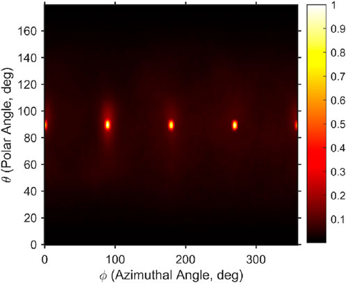
Figure 4. Time-averaged, normalized orientation density of water molecules for case B. The distribution is plotted as a function of polar and azimuthal angles, representing the angular preferences of the water orientation vectors. Simulations were performed using the Zhu–Philpott (ZP) potential.

To further examine angular distributions, we compute marginal orientation distributions, which are presented in a polar overlay plot. These are calculated by integrating over one angle to project onto the other. Azimuthal distribution (red curve in Figure 5) and as per Equation 14 is estimated by,

$P_{\varphi }\left({\varphi }_k\right)={\displaystyle \sum _{j=1}^{N_{\theta }}}f\left({\theta }_j,{\varphi }_k\right),{\widehat{P}}_{\varphi }\left({\varphi }_k\right)=\frac{P_{\varphi }\left({\varphi }_k\right)}{\mathit{max}\left(P_{\varphi }\right)}(14)$

Figure 5

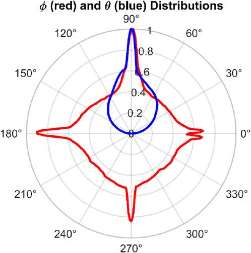
Figure 5. Spherical distribution of water orientation vectors in the water film above platinum for case B. The orientation vectors are represented in spherical coordinates, capturing their directional distribution relative to the surface normal. The system is modeled using the Zhu–Philpott (ZP) potential.

Polar distribution (blue curve in Figure 5) as per Equation 15:

$P_{\theta }\left({\theta }_k\right)={\displaystyle \sum _{k=1}^{N_{\varphi }}}f\left({\theta }_j,{\varphi }_k\right),{\widehat{P}}_{\theta }\left({\theta }_j\right)=\frac{P_{\theta }\left({\theta }_j\right)}{\mathit{max}\left(P_{\theta }\right)}(15)$

The normalized projections, ${\widehat{P}}_{\varphi }$ and ${\widehat{P}}_{\theta }$, are plotted in polar coordinates. The azimuthal distribution ${\widehat{P}}_{\varphi }$ is plotted as a function of the azimuthal angle $\varphi$, while the polar distribution ${\widehat{P}}_{\theta }$ originally defined over $\left[0°,180°\right]$, is mapped onto a synthetic 360° angular axis to allow consistent radial representation. The resulting plot, shown in Figure 5, offers an intuitive comparison of directional biases in molecular orientation. For clarity in subsequent discussions, we refer to the 2D orientation heatmap $f\left(\theta ,\varphi \right)$ as the orientation density plot, and the marginal angular distribution plot as the overlay plot.

The overlay plot Figure 5 shows the preferential orientation of water molecules in selected directions mainly due to the lattice structure of the platinum and its influence on water molecules.

2.5 Studies with equivalent LJ potential

While the Zhu–Philpott (ZP) potential provides a detailed and accurate description of the interaction between water molecules and metallic surfaces by incorporating image charge effects, isotropic repulsion, and anisotropic attraction, it is computationally intensive and not readily applicable to large-scale molecular dynamics (MD) simulations. Therefore, it is often desirable to approximate this complex potential using simpler forms such as Lennard-Jones (LJ) or Morse potential. In this study, we begin by estimating the parameters of an LJ 12-6 potential that best reproduces the effective interaction described by the ZP potential.

The decomposition of the ZP potential is shown in Figure 6a, where the dashed lines represent individual components: the image charge interaction (conduction electron potential), isotropic repulsion, and anisotropic attraction. The solid purple line indicates the total interaction energy, $U_{total}$, obtained by summing all three contributions. Using a nonlinear least-squares fitting procedure, we estimate the LJ parameters that best match this total interaction energy. The fitted parameters are:

${ϵ}_{O-Pt}=3.3939kcal/mol,{\sigma }_{O-Pt}=0.22273nm,{ϵ}_{H-Pt}=2.1953kcal\backslash mol,{\sigma }_{H-Pt}=0.18698nm$

Figure 6

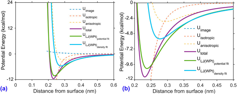
Figure 6. Decomposition of the water–platinum interaction potential based on the Zhu–Philpott (ZP) model. (a) Full view of the potential energy components as a function of the distance from the platinum surface. (b) Zoomed-in view highlighting the attractive well region. The total interaction energy $U_{total}$ (solid purple) is shown alongside its constituent components: image interaction $U_{image}$ (blue dashed), isotropic repulsion $U_{isotropic}$ (orange dashed), and anisotropic attraction $U_{anisotropic}$ (yellow dashed). Also shown are two Lennard-Jones-based approximations for water–platinum interaction: a potential-fit curve (green) and a density-fit curve (light blue).

This fitted potential is plotted as the green solid line in Figure 6a and labeled $U_{LJ\left(W-Pt\right)potentialfit}$. A magnified view of the interaction range from 0.2 to 0.5 nm is shown in Figure 6b to highlight the differences between the ZP potential and its LJ fit. Although the LJ fit closely resembles the ZP curve, it cannot fully capture the complex shape of the ZP potential. Consequently, MD simulations using this fitted LJ potential produce artificially elevated water densities near the surface—almost twice the values reported in the literature.

The fitting was performed by minimizing objective function as per the Equation 16:

$Objective={\displaystyle \sum _{k=1}^{N_z}}{\left[U_{LJ}^{fit}\left(z_k\right)-U_{total}\left(z_k\right)\right]}^2(16)$

Here, $Nz$ is the number of discrete height points considered, $U_{LJ}^{fit}\left(z_k\right)$ is the LJ energy at height $z_k$, $U_{total}\left(z_k\right)$ is the corresponding ZP total energy at $z_k$.

Although the potential-fit LJ curve visually aligns well with the original ZP potential across the interaction range, MD simulations using this fit produced unphysical results, most notably significantly elevated water densities near the platinum surface, with nearly twice the values reported in the literature. This suggests that a visually accurate energy profile alone may not be sufficient to reproduce realistic interfacial water structuring. To improve physical realism, particularly in reproducing the water structure near the surface, we repeated the LJ fitting using water density profiles as the optimization target instead of the potential energy. In this second optimization, we compared the simulated water density profiles against those reported in the literature (Chen et al., 2018). The resulting LJ parameters were:

${ϵ}_{O-Pt}=0.926kcal/mol,{\sigma }_{O-Pt}=0.270nm,{ϵ}_{H-Pt}=0.563kcal/m\text{ol},{\mathrm{\sigma }}_{H-Pt}=0.255nm$

In fact, these parameters are same as the one for anisotropic potential part of the ZP potential with the scaling factor as 1. This optimized set is plotted in light blue in Figure 6 and labeled $U_{LJ\left(WPt\right)densityfit}$. The resulting density distribution of oxygen atoms near the platinum surface is shown in Figure 7. It exhibits excellent agreement with literature data, especially within the first 0.5 nm from the surface, capturing both the magnitude and location of the density peaks. The optimization process employed the same nonlinear least-squares framework as the potential fitting, but with density profiles as the target observable instead of interaction energies.

Figure 7

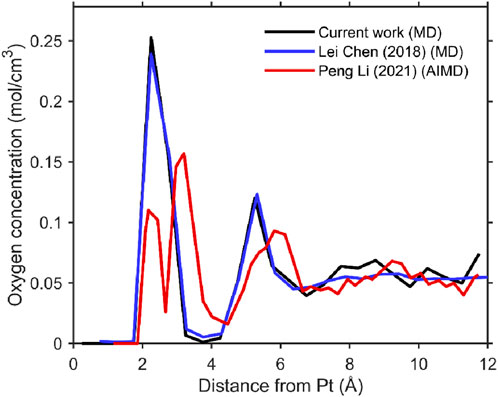
Figure 7. Oxygen density distribution as a function of distance from the platinum surface for case B using the equivalent (density fitted) Lennard-Jones potential. The results from the current MD simulation (black) are compared with prior molecular dynamics results by Chen (2018) (blue) and ab initio molecular dynamics (AIMD) results by Li (2021) (red).

It may appear that the density distributions obtained from our classical MD simulations differ from those reported in AIMD studies in the literature, particularly in the presence of more pronounced or fluctuating peak structures. This discrepancy is likely due to several factors inherent to the AIMD methodology: notably, the limited number of water molecules typically used (often only 12–48), the relatively short sampling duration (∼10 ps), and the use of finer spatial bin widths (0.1–0.2 Å) for density averaging. In contrast, our MD simulations incorporate significantly larger system sizes, longer trajectories, and coarser bin widths (e.g., 0.5 Å), which collectively contribute to smoother and more statistically converged density profiles. These methodological differences can result in apparent variations in the resolution and sharpness of interfacial layering, but do not necessarily indicate fundamental disagreement in physical behavior.

The results of this study demonstrate that the equivalent Lennard-Jones (LJ) potential, particularly the version optimized to match the density distribution (i.e., the “density-fit” LJ potential), is sufficient to reproduce the structural features of interfacial water in classical molecular dynamics (MD) simulations. This simplified potential effectively captures key characteristics such as the magnitude and location of the density peaks near the platinum surface, showing excellent agreement with both previous MD studies and ab initio molecular dynamics (AIMD) results in the near-surface region. While it does not fully replicate the complex shape of the original Zhu–Philpott (ZP) potential, its computational efficiency and accuracy in modeling structural behavior make it a practical and reliable choice for large-scale classical MD studies. However, for investigations those require detailed insight into electronic effects, polarization, or highly accurate energetics, particularly at the quantum mechanical level, a more rigorous approach such as AIMD is warranted. AIMD remains the gold standard for capturing the fine-grained physics of water–metal interfaces, even though with significant computational cost and system size limitations.

Having validated the water–platinum interaction using the density-fitted Lennard-Jones potential $U_{LJ\left(WPt\right)densityfit}$, we then explored how different thermostating strategies affect the structure and dynamics of interfacial water. To do this, we systematically varied the thermal control applied to both the water molecules and the platinum substrate. Four distinct simulation cases were designed, as summarized in Table 1, allowing us to isolate and analyze the individual and combined effects of thermostating the wall and the water. This structured approach follows a design of experiments framework to ensure comprehensive and comparative evaluation across the different thermal boundary conditions.

As outlined in Table 2, we designed four distinct simulation cases to systematically examine the influence of thermostating strategies on the structural and dynamical behavior of interfacial water. In case A, both the platinum atoms and water molecules are thermostated using independent Nosé–Hoover thermostats maintained at 300 K. Case B is identical to case A, except the thermostat is applied only to the water molecules, with the platinum wall left un-thermostated. In case C, neither the platinum atoms nor the water molecules are subjected to any thermostats during the production phase, enabling the system to evolve under NVE dynamics. Case D mirrors case A but omits the thermostat for water molecules, allowing only the platinum atoms to be temperature-controlled.

Table 2

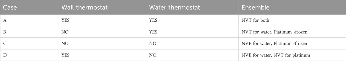
Table 2. Study cases to understand the effects of wall thermostating.

To ensure consistent equilibration across all cases and avoid numerical instabilities, thermostats were applied to water molecules during an initial 0.5 ns equilibration period in all simulations. This step mitigates the impact of integration errors and ensures thermal relaxation. In cases where water thermostats are disabled during the production run (e.g., cases C and D), water molecules subsequently evolved without direct thermal coupling for another 0.5 ns under specified conditions.

In scenarios where the thermostating of the platinum wall is omitted (cases B and C), the platinum atoms are constrained to their equilibrium positions via a harmonic tethering potential. This approach prevents unphysical drift or diffusion of the wall atoms while allowing limited thermal fluctuations. The spring constant for the tether was estimated by equating the harmonic potential energy to the mean thermal energy at the target temperature, with a maximum displacement capped at 0.5 Å. This yielded a value of approximately 50 eV/Ų, which, although higher than typically used, is justified for simulations where temperatures may transiently rise above 300 K.

Based on this design matrix and the simulation methodology detailed in the Methods section, a comprehensive set of molecular dynamics simulations was performed. The resulting data and analyses are presented and discussed in the following section.

3 Results and discussion

This section presents the effects of different thermostating methods on the structural and dynamic properties of water near a platinum surface. Four different cases were simulated, each with a different combination of thermal control applied to the wall and the water, as mentioned in Table 1.

3.1 Water orientation distributions

Figure 8 shows how the orientation of water molecules changes depending on the thermostating case. Each plot presents the normalized density of dipole orientation vectors in terms of polar and azimuthal angles. For cases A and B (Figures 8a,b), the density distribution seems to be concentrated near the crystallographic directions of the platinum (e.g., 0°, 90°, 180° azimuthally). In contrast, cases C and D (Figures 8c,d), exhibit a broader and more dispersed distribution, which is primarily attributed to elevated water temperatures in the absence of thermostating.

Figure 8

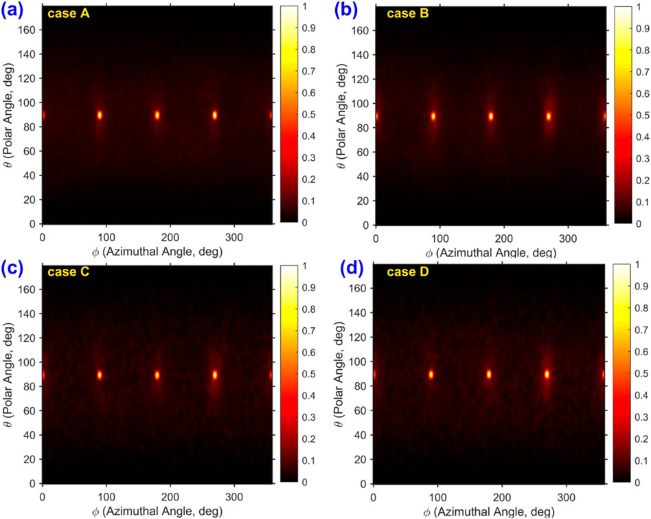
Figure 8. Time-averaged, normalized orientation density of water molecules in spherical coordinates for all four simulation cases. The distribution is shown as a function of polar angle θ and azimuthal angle ϕ for: (a) case (A) wall and water thermostated, (b) case (B) only water thermostated, (c) case (C) no thermostats applied, and (d) case (D) only wall thermostated. The color scale indicates the normalized density of orientation vectors, highlighting the angular preferences of water dipoles under different thermostating conditions.

Root-mean-square displacement (RMSD) analysis indicates that the platinum atoms exhibit minimal thermal motion, with a maximum displacement of only 0.134 Å. This minimal fluctuation implies that the platinum surface remains structurally stable and has limited influence on the dynamic behavior of the overlying water layers. These observations collectively suggest that water temperature, governed by its thermostating condition, plays a more dominant role in determining the orientation and spatial distribution of water molecules than the thermal state of the platinum substrate.

These observations are further visualized by the polar overlay plots in Figure 9, which presents the angular distributions of water dipole orientations under various thermostating conditions, using normalized spherical coordinates. The azimuthal angle φ (red curves) shows pronounced peaks near 0°, 90°, 180°, and 270° for all cases, suggesting a strong preferential in-plane alignment of dipoles relative to the platinum surface lattice orientation. This pattern aligns well with the underlying surface symmetry and expected in-plane ordering near hydrophilic interfaces.

Figure 9

Figure 9. Polar representation of water orientation vector distributions in the water film above platinum for different simulation cases. The normalized distributions of azimuthal angle ϕ (in red) and polar angle θ (in blue) are shown for: (a) case (a) wall and water thermostated, (b) case (b) only water thermostated, (c) case (c) no thermostats applied, and (d) case (d) only wall thermostated. These plots highlight the angular preferences in molecular orientation under varying thermal boundary conditions.

The polar angle θ (blue curves) remains sharply centered around 90° indicating that the dipoles predominantly lie parallel to the surface. Analyzing all these cases, based on Figure 9, there are no distinct features indicating the differences in water molecular orientation. However, cases A and B show a better distribution of water molecules in the azimuthal direction compared with cases C and D. This can be seen by having normalized density above 0.4 for angles 120, 150, 330, 300, etc.

3.2 Density profiles

Figure 10 presents oxygen number density profiles of SPC/E water adjacent to Pt (111) for four thermostat configurations—A (wall thermostated, water thermostated), B (wall fixed, water thermostated), C (wall fixed, water not thermostated), and D (wall thermostated, water not thermostated)—alongside reference curves from classical MD (Chen et al., 2018) and AIMD (Li et al., 2021). All cases exhibit a first hydration peak near 2.5–3.0 Å, but its amplitude depends strongly on how heat is handled at the interface: the fixed-wall cases B and especially C display an elevated first peak and deeper following troughs, indicative of over-structuring caused by an atomically rigid, non-dissipative substrate, whereas the wall-thermostated cases A and D yield moderate peak heights and shallower troughs that more closely track the literature in both peak position and amplitude.

Figure 10

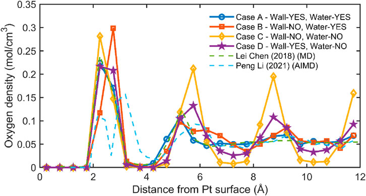
Figure 10. Oxygen density near Pt (111) under different thermostating schemes. Profiles are computed with Δz = 0.5 Å, referenced to the outermost Pt (111) plane (z = 0). Cases: A (Wall-YES, Water-YES, blue ○), B (Wall-NO, Water-YES, orange □), C (Wall-NO, Water-NO, yellow ◇), D (Wall-YES, Water-NO, purple ★). Literature curves from (Chen et al., 2018) (green dashed, MD) and (Li et al., 2021) (blue dashed, AIMD) are shown for context. Dual-thermostating (A) and wall-only thermostating (D) produce layering most consistent with MD/AIMD, whereas non-thermostated walls ,(B, C) show stronger layering (higher first peak, deeper troughs).

The second-layer feature at ∼5–6 Å is most consistent with prior MD/AIMD in case A, is slightly broader and lower in case D (reflecting greater fluid mobility when the water is unthermostated), and is exaggerated in case C, which also shows longer-ranged oscillations and slower decay to bulk, consistent with insufficient thermal damping when neither the wall moves nor the water is thermostated. Beyond ∼10 Å, all profiles approach the expected bulk density (∼0.055 mol cm^-3). Taken together, these trends support the physical picture that allowing wall vibrations provides a realistic thermal and mechanical coupling that suppresses artificial ordering in the first few layers; thus, for quantitative inference about interfacial structure, dual thermostating (A) or wall-only thermostating (D) is preferable, while fixed-wall setups (B, C) should be used with caution because they can overstate layering and misrepresent the near-wall microstructure.

The structuring of interfacial water is highly sensitive to the dynamic nature of the substrate and the thermal treatment of the fluid. Simulations with fixed walls (Wall-NO) tend to exaggerate water structuring, while dynamic walls (Wall-YES) yield more physically realistic density profiles. Among all cases, case A (Wall-YES, Water-YES) provides the best agreement with literature and offers a robust configuration for modeling interfacial systems in molecular simulations. Figure 11 presents a representative snapshot of the interfacial water structure above a platinum (Pt) surface for case A, where both the platinum atoms and water molecules are time-integrated and thermostated (Wall-YES, Water-YES). The Pt slab, shown on the left in dark gray spheres, is in contact with a slab of SPC/E water. Oxygen atoms are depicted in red, hydrogen in white, and the overlaid black line corresponds to the time-averaged oxygen density profile as a function of distance from the Pt surface.

Figure 11

Figure 11. Snapshot of the interfacial water structure above the platinum surface, overlaid with the oxygen density profile, for case A. The platinum slab (left, dark gray spheres) is shown in contact with a water film, where oxygen atoms are depicted in red, hydrogen in white. The black line represents the time-averaged oxygen density distribution as a function of distance from the Pt surface. Layering of water molecules is clearly visible, consistent with the peaks in the density profile.

To gain deeper insight into the structural organization of water within the interfacial region, we performed a localized analysis of the radial distribution function (RDF) within two distinct spatial slices corresponding to the first and second hydration layers observed in the oxygen density profile. Slice 1, representing the first hydration layer, spans from z = 1.55 Å to 4.03 Å, capturing the region surrounding the first density peak. Slice 2, corresponding to the second hydration layer, covers the range from z = 4.05 Å to 7.05 Å, aligned with the second peak in the profile. The RDFs calculated within these slices provide a detailed view of the local molecular arrangement and hydrogen bonding structure within each layer. The resulting distributions are presented in Figure 12, offering a comparative understanding of the short-range order and spatial correlations of water molecules in the near surface versus sub-bulk region.

Figure 12

Figure 12. Radial distribution functions (RDF) of oxygen atoms in interfacial water for different thermostating cases. (a) Averaged RDF g(r) in Slice 1 (near the platinum surface, z = 1.55Å to 4.03Å) for cases (A–D). (b) Averaged RDF g(r) in Slice 2 (further from the surface, z = 4.05Å to 7.05Å) for the same cases. (c) Zoomed-in view of the boxed region from panel (a) focusing on the second coordination shell. (d) Zoomed-in view of the boxed region from panel (b) highlighting subtle variations in RDF peak positions and magnitudes. All simulations show characteristic peaks near 0.275 nm, with differences in structural ordering depending on the thermostating scheme.

3.3 Radial distribution functions (RDFs)

Panel (a) of Figure 12 shows the RDF g(r) within Slice 1 for cases A–D. All four cases exhibit a strong first peak near ∼0.275 nm, consistent with the typical oxygen–oxygen distance in bulk water. However, case B (Wall-NO, Water-YES) shows the highest RDF peak (∼22), indicating extremely sharp local ordering. This behavior is attributed to the fixed Pt wall, which provides a rigid and smooth interface, allowing for tight and structured packing of the first water layer. In contrast, case C (Wall-NO, Water-NO) shows the lowest peak magnitude, likely due to a lack of thermal regulation, leading to increased molecular agitation and a more disordered interface. Cases A (Wall-YES, Water-YES) and D (Wall-YES, Water-NO) show intermediate ordering, indicating that wall motion dampens over-structuring while preserving hydration shell features. These exaggerated structural features are confined to the near-surface layer. For simulations concerned with interfacial mechanisms at the molecular scale (e.g., adsorption, hydration layer stability), such artifacts must be avoided by including wall thermostating. However, for transport modeling or studies not resolving interfacial fine structure, the simplification of using fixed or non-thermostated walls is justified.

Panel (c) provides a zoomed-in view of the second coordination shell (0.35–0.6 nm). Here, case A shows a distinct second peak, suggesting a well-defined intermediate-range structure. Case C, again, exhibits a more smeared and broad distribution, reflecting weaker structuring beyond the first shell. Panel (b) displays the RDFs within Slice 2. The overall peak heights are reduced (∼13 at most), indicating diminished ordering compared to the near-surface region. Still, all cases retain a primary peak at ∼0.275 nm, indicative of persistent short-range order even at greater distances from the interface. As seen in panel (d) (zoomed view), the differences between cases are subtler than in Slice 1. However, case A consistently maintains smoother, broader peaks, suggesting that dual thermostating helps preserve moderate structuring while avoiding rigid over-confinement. Case B still shows relatively sharp peaks, indicating that fixed walls continue to influence molecular packing beyond the immediate interface.

These findings confirm that wall dynamics and water thermostating play critical roles in determining the structural organization of interfacial water:

• Fixed walls (Wall-NO) lead to excessive local ordering and unnaturally sharp RDF peaks, especially in the first hydration shell.

• Dynamic walls (Wall-YES) introduce vibrational motion that dampens these effects, resulting in more physically realistic structures.

• Thermostating water molecules helps preserve consistent thermal energy distribution, especially critical in subsurface regions (Slice 2).

The RDF analysis reveals how subtle changes in thermostating schemes significantly affect both short- and medium-range water structuring near solid surfaces. Among all tested conditions, case A (Wall-YES, Water-YES) provides the most balanced and physically representative behavior, preserving hydration shell structure without artificial over-ordering. This reinforces the earlier conclusions drawn from the density profile and visual inspection and supports the use of case A for realistic interfacial water modeling in molecular dynamics studies.

It is important to note that the RDFs shown in Figure 12 are computed from spatial slices near the platinum surface and thus do not represent bulk-like spherical symmetry. Due to the proximity of the wall, the sampling volume available for constructing spherical shells around each atom is truncated. However, the RDF calculation assumes a full spherical shell volume $4\pi r^{2}dr$, leading to inflated peak heights near the interface. This geometric bias arises because fewer particles contribute to the shell, but the normalization does not account for the reduced sampling domain. As a result, RDF values particularly in the first hydration layer (Slice 1) may overestimate the actual degree of structural ordering. This artifact is a well-known limitation of RDF analysis near interfaces and does not necessarily indicate stronger water–water correlations. Care must be taken in interpreting absolute peak heights in these cases; relative comparisons between simulation conditions (e.g., cases A–D) remain valid and informative when analyzed within the same geometric constraints.

3.4 Temperature evolution

Figure 13 illustrates the temporal evolution of the platinum slab temperature $T_{Pt}$ over the course of the simulation for cases A and D. In both cases, the platinum atoms are subjected to a thermostat, ensuring active thermal regulation. As shown, the instantaneous temperatures fluctuate slightly due to natural thermal motion but remain well-centered around the target temperature of 300 K, confirming effective and stable thermal control of the substrate.

Figure 13

Figure 13. Temperature evolution of the platinum slab over time for cases A–D. The instantaneous temperature of Pt atoms ($T_{Pt}$) is plotted as a function of simulation time. Case A (blue) corresponds to both wall and water thermostated, case B (orange) to only water thermostated, case C (yellow) to neither thermostated, and case D (purple) to only the wall thermostated. In all cases, the platinum temperature fluctuates around ∼300 K, confirming stable thermal control of the substrate across the tested configurations.

The thermal stability of the Pt wall is particularly important in simulations involving interfacial heat transfer and molecular layering, as it avoids artificial heating or cooling that could influence fluid behavior at the interface. The temperature profiles demonstrate that wall thermostating is robust and consistent across both cases, regardless of whether the water phase is thermostated (case A) or not (case D).

Figure 14 presents the temperature trajectories of water molecules for all four simulation cases over a 0.5 ns simulation period. Distinct differences emerge depending on whether the water molecules are thermostated:

• In case A (black) and case B (orange), where the water phase is directly coupled to a thermostat, the water temperature remains stable around 300 K throughout the simulation. These results validate the thermostat’s performance in maintaining a consistent thermal environment within the fluid.

• In case C (blue) and case D (red), where water is not thermostated, the temperature increases steadily over time. This trend arises due to energy transfer from the platinum slab, which is maintained at 300 K, to the adjacent water molecules. In the absence of a thermostat, the water accumulates thermal energy from wall-fluid interactions, resulting in a gradual and uncontrolled rise in temperature.

Figure 14

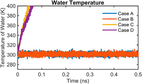
Figure 14. Temporal evolution of water temperature in all four simulation cases. The instantaneous temperature of water molecules is shown over a 0.5 ns simulation period for case A (black), case B (orange), case C (blue), and case D (red). In cases A and B, where the water is thermostated, the temperature remains stable around 300 K. In cases C and D, where the water is not thermostated, a steady temperature increase is observed due to energy exchange with the platinum substrate and due to the absence of thermostat.

Therefore, for cases C and D, the structural analyses, such as density profiles and radial distribution functions (RDFs) are computed using only the initial 25 ps of the simulation. This early-time window ensures that the results reflect a thermally equilibrated state prior to significant temperature drift, thereby enabling meaningful comparisons with thermostated cases and avoiding artifacts introduced by thermal non-equilibrium over longer timescales.

3.5 Temperature profile of water

Figure 15 presents the spatial temperature distribution of water molecules in proximity to the platinum wall for cases A and B, each employing different thermostating strategies. In both cases, the water molecules are maintained at 300 K using a Nosé–Hoover thermostat, while the platinum wall atoms are thermostated in case A and not in case B.

Figure 15

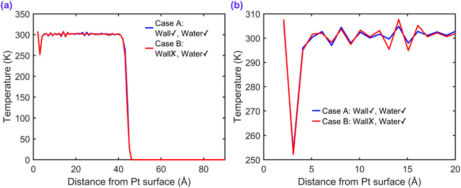
Figure 15. Time-averaged temperature profiles of water molecules along the direction normal to the platinum surface (z-direction) for two thermostating configurations: case A (Wall✓, Water✓) and case B (Wall✗, Water✓). (a) Full-domain temperature profile showing the influence of wall thermostating on the entire water slab. (b) Zoomed-in view near the solid–liquid interface revealing thermal equilibration details within 20 Å from the platinum surface.

As shown in Figure 15a, the bulk region of the water slab maintains a nearly uniform temperature around 300 K in both cases, indicating effective control by the water-phase thermostat. However, a slight difference arises near the platinum surface at approximately around 1.2 nm. Case A exhibits a smooth temperature transition from the solid to the liquid, reflecting efficient interfacial thermal equilibration. In contrast, case B shows a distinct thermal gradient near the wall and a significantly lower temperature in the interfacial region, especially evident in Figure 15b.

This localized cooling effect in case B can be attributed to the lack of thermal coupling from the platinum atoms. Without a thermostat or dynamic motion in the wall, vibrational energy transfer at the interface is suppressed, resulting in under-heated interfacial water layers. These findings highlight the importance of thermostating the solid phase to maintain realistic interfacial thermal conditions, particularly in simulations targeting heat transfer, evaporation, or confined liquid behavior.

3.6 Water–platinum interaction energies

To assess the energetic stability of the water–platinum interface under different thermostating conditions, we tracked the total interaction energy between water molecules and Pt atoms over time for all four cases, as shown in Figure 16. In cases A (Wall-YES, Water-YES), B (Wall-NO, Water-YES), and D (Wall-YES, Water-NO), the water–Pt interaction energy remains consistently negative and stable throughout the 0.5 ns simulation. This suggests that, despite differences in wall dynamics or fluid thermostating, these configurations maintain an interaction with the platinum surface without significant fluctuations in energetic interaction.

Figure 16

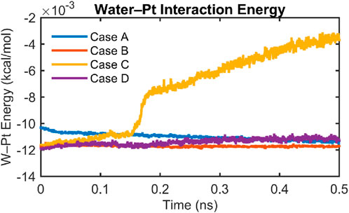
Figure 16. Temporal evolution of the water–platinum interaction energy for all four simulation cases. The interaction energy is plotted as a function of simulation time for case A (blue), case B (orange), case C (yellow), and case D (purple). cases A, B, and D exhibit stable interaction energies throughout the 0.5 ns simulation, indicating well-equilibrated water–Pt interfaces. In contrast, case C (Wall-NO, Water-NO) shows a sharp increase in interactive energy after ∼0.18 ns, reflecting a loss of interfacial stability due to uncontrolled heating of water in the absence of thermostating. This further justifies limiting structural analyses in case C to the initial 25 ps.

In stark contrast, case C (Wall-NO, Water-NO) exhibits a sudden and sustained increase in interaction energy starting around 0.18 ns. This shift indicates a gradual weakening of water–Pt interactions, caused by uncontrolled heating of the water phase in the absence of a thermostat. As the water temperature rises (as previously shown in Figure 14), thermal agitation overcomes the binding affinity of water molecules to the surface, leading to partial desorption or restructuring at the interface. This energetic instability further supports the decision to restrict structural analysis (e.g., density profiles and RDFs) for case C to the first 25 ps, where the interface remains relatively undisturbed and physically meaningful comparisons to other cases are still valid.

The interaction energy behavior highlights the importance of thermostating at least one phase in interfacial simulations to ensure stability. While case D (no water thermostat) does not exhibit instability within the 0.5 ns window, likely due to thermal buffering from the thermostated Pt wall, case C lacks both energy dissipation mechanisms and consequently drifts toward nonphysical states. Overall, case A emerges again as the most thermodynamically stable and physically consistent configuration, maintaining steady interfacial energy while preserving structural integrity in both the solid and fluid phases. This suggests that thermostating is necessary to maintain interfacial stability over longer timescales. However, for short simulations or when only coarse-grained averages (e.g., diffusivity or thermal fluxes) are of interest, thermostating only the water may suffice.

3.7 Structural snapshots

Figure 17 shows side-view snapshots of the equilibrated water–platinum interface for all four simulation cases, captured at the end of a 0.5 ns simulation period. Each panel corresponds to a different thermostating configuration: (a) case A–Wall-YES, Water-YES, (b) case B–Wall-NO, Water-YES, (c) case C–Wall-NO, Water-NO, (d) case D–Wall-YES, Water-NO. In all configurations, platinum atoms (dark gray) form the bottom layer, in contact with a slab of water composed of oxygen atoms (red) and hydrogen atoms (white). Despite similar initial water loading, noticeable structural differences emerge across the cases due to the distinct thermal treatments applied to the wall and water.

Figure 17

Figure 17. Side-view snapshots of the equilibrated water–platinum interface for the four simulation cases: (a) Case (A) wall and water thermostated, (b) Case (B) only water thermostated, (c) Case (C) no thermostats applied, and (d) Case (D) only wall thermostated. At this scale, the panels appear visually similar, with Case C showing slightly more dispersed vapor molecules. The figure is intended as a qualitative visualization aid to complement the quantitative analyses. The structural and thermodynamic differences between cases are more rigorously captured in the oxygen density profiles (Figure 10), orientation distributions (Figures 8, 9), radial distribution functions (Figure 12), and interaction energies (Figure 16).

In case A, where both the wall and water are thermostated, the water film maintains a dense and well-layered structure near the interface. The stratified arrangement of oxygen atoms suggests stable hydration layers, consistent with the density profile and RDF results. Case B, with a fixed wall and thermostated water, shows a slightly more compressed water structure at the interface. The rigidity of the wall leads to enhanced ordering in the immediate contact layer, but layering beyond the surface appears less pronounced than in case A, possibly due to reduced surface vibrations.

In case C, where neither the wall nor water are thermostated, the interfacial structure becomes visibly less organized, and several water molecules are seen rising above the main liquid layer. This dispersal is consistent with the observed temperature increase and weakening of water–Pt interactions in previous analyses (Figures 10, 14). Without thermal regulation, energy accumulates, resulting in reduced layering and partial desorption of water molecules. Case D displays intermediate behavior, similar to case A but with a slightly looser packing of water molecules. The presence of a thermostated, dynamic wall provides energy dissipation, but the absence of thermostating on water allows for mild temperature drift, slightly impacting structural definition over long timescales.

These snapshots reinforce that the thermostating strategy directly impacts the microscopic structure of interfacial water. Case A remains the most stable and physically representative configuration, showing well-preserved layering and strong adsorption. In contrast, case C demonstrates how the absence of thermal control can degrade interfacial integrity, even in the absence of external perturbations. Visual confirmation of structural degradation in case C also validates the decision to limit its structural analysis to early simulation times, as discussed in previous sections.

4 Discussion on results, limitations, and future directions

The results presented in this study demonstrate that the choice of thermostating strategy and interaction potential fundamentally alters the interfacial structure, orientation, and energetics of water near platinum. Thermostating both the water and the solid (Case A) yielded interfacial density layering and orientation distributions that are in closest agreement with earlier MD and AIMD studies (Gereben and Pusztai, 2011; Sakamaki et al., 2011a; 2011b; Zhu, 2013; Chen et al., 2018; Zhang et al., 2019; Li et al., 2021; Groß and Sakong, 2022b; Zheng et al., 2024), thereby confirming the importance of including vibrational motion of the wall for realistic interfacial modeling. These findings are consistent with experimental surface-sensitive techniques such as X-ray reflectivity (XRR) and sum-frequency generation (SFG), which report distinct hydration layering and preferential dipole orientations at metal–water boundaries (Fenter and Lee, 2014; Guo et al., 2018; Sanders and Petersen, 2019).

At the same time, the results reveal practical guidelines for simulation fidelity: (i) fixed walls or un-thermostated systems can artificially enhance ordering or lead to unstable dynamics, while (ii) dual thermostating provides a balanced and physically meaningful representation of thermal coupling at interfaces. Thus, the study clarifies when simplified Lennard-Jones potentials and computational shortcuts may be acceptable, and when detailed models such as the Zhu–Philpott (ZP) potential and explicit wall dynamics are essential for accuracy.

4.1 Limitations

Despite the detailed atomistic resolution, this work is constrained to equilibrium simulations at a single temperature and planar platinum (111) surfaces. Phenomena such as evaporation, nucleation, or interfacial charge transfer—which are highly relevant to catalysis and energy storage—are not directly captured. Additionally, the simulation timescale (∼1 ns) and system size (∼2,200 water molecules) are sufficient for resolving short- and medium-range structuring but cannot capture rare events or longer diffusive transport processes.

4.2 Future directions

Building on these findings, several research avenues emerge. First, extending the simulations to nonequilibrium conditions (e.g., applying thermal gradients) could provide molecular-level insights into nanoscale heat transfer and phase change, bridging toward the macroscopic phenomena referenced in the introduction. Second, coupling atomistic results with continuum heat and mass transfer models would enable multiscale predictions relevant to boiling, condensation, and thermal management applications. Finally, the role of surface chemistry and heterogeneity (e.g., alloyed or functionalized surfaces) could be investigated to generalize the observed trends beyond platinum.

5 Conclusion

This work clarifies the intertwined roles of thermostating strategies and interaction potentials in governing the structural and energetic behavior of interfacial water near metal surfaces. Through systematic molecular dynamics simulations of SPC/E water in contact with a platinum (111) surface, we provide direct evidence that both the dynamic state and thermal regulation of the substrate substantially influence the fidelity of interfacial modeling. When the platinum wall is left un-thermostated or held rigid, artificial cooling and exaggerated ordering of water molecules emerge manifesting as nonphysical layering and orientation artifacts within the first solvation layer. These effects are localized within ∼0.5 nm of the surface but are critical for simulations that seek to resolve molecular orientation, dipole alignment, or hydrogen bonding topology.

We also show that the widely used Lennard-Jones (LJ) potential, when carefully fitted to reproduce either interaction energy profiles or density distributions from the more rigorous Zhu-Philpott (ZP) potential, can recover major features of interfacial structuring particularly in terms of oxygen layering. However, the LJ approximation fails to capture angular orientation characteristics intrinsic to anisotropic interactions encoded in the ZP framework. This result highlights the limits of simplified interaction models, especially when simulating phenomena where electronic image forces and directional bonding matter.

Importantly, our findings help define a practical fidelity-cost trade-off in interfacial simulations. For simulations aiming to capture fine-scale interfacial physics such as electrochemical double-layer behavior, contact line dynamics, or nanoscale heat transfer both dual thermostating and a high-fidelity potential (e.g., ZP) are essential. In contrast, for studies focused on bulk transport, long-range energy dissipation, or macroscopic wetting behavior, simplified potentials and water-only thermostats suffice, delivering computational efficiency without compromising global accuracy.

By identifying where simulation choices begin to distort physical realism, this work provides actionable guidance for the molecular modeling community. The framework and physical insights presented here are broadly applicable across interfacial systems, including those involving water-oxide, polymer-liquid, or biological-material interfaces, where thermal gradients and anisotropic interactions shape interfacial organization. These conclusions not only resolve ambiguities in current simulation practices but also establish a benchmark for method selection in future computational investigations of soft matter at interfaces.

Data availability statement

The data supporting the findings of this study are available from the corresponding author upon reasonable request. All other relevant materials are included within the article.

Author contributions

SY: Investigation, Software, Resources, Supervision, Funding acquisition, Project administration, Writing – review and editing, Conceptualization, Writing – original draft, Methodology, Formal Analysis, Data curation, Visualization, Validation.

Funding

The author(s) declare that no financial support was received for the research and/or publication of this article.

Conflict of interest

The author declares that the research was conducted in the absence of any commercial or financial relationships that could be construed as a potential conflict of interest.

Generative AI statement

The author(s) declare that no Generative AI was used in the creation of this manuscript.

Any alternative text (alt text) provided alongside figures in this article has been generated by Frontiers with the support of artificial intelligence and reasonable efforts have been made to ensure accuracy, including review by the authors wherever possible. If you identify any issues, please contact us.

Publisher’s note

All claims expressed in this article are solely those of the authors and do not necessarily represent those of their affiliated organizations, or those of the publisher, the editors and the reviewers. Any product that may be evaluated in this article, or claim that may be made by its manufacturer, is not guaranteed or endorsed by the publisher.

References

Arblaster, J. W. (1997). Crystallographic properties of platinum. Platin. Met. Rev. 41, 12–21. doi:10.1595/003214097x4111221

CrossRef Full Text | Google Scholar

Berendsen, H. J. C., Grigera, J. R., and Straatsma, T. P. (1987). The missing term in effective pair potentials. J. Phys. Chem. 91, 6269–6271. doi:10.1021/j100308a038

CrossRef Full Text | Google Scholar

Carrasco, J., Hodgson, A., and Michaelides, A. (2012). A molecular perspective of water at metal interfaces. Nat. Mater. 11, 667–674. doi:10.1038/nmat3354

PubMed Abstract | CrossRef Full Text | Google Scholar

Chen, L., Chen, P.-F., Li, Z.-Z., He, Y.-L., and Tao, W.-Q. (2018). The study on interface characteristics near the metal wall by a molecular dynamics method. Comput. Fluids 164, 64–72. doi:10.1016/j.compfluid.2017.03.013

CrossRef Full Text | Google Scholar

Drost-Hansen, W. (1969). STRUCTURE OF WATER NEAR SOLID INTERFACES. Ind. Eng. Chem. 61, 10–47. doi:10.1021/ie50719a005

CrossRef Full Text | Google Scholar

Fenter, P., and Lee, S. S. (2014). Hydration layer structure at solid–water interfaces. MRS Bull. 39, 1056–1061. doi:10.1557/mrs.2014.252

CrossRef Full Text | Google Scholar

Gereben, O., and Pusztai, L. (2011). On the accurate calculation of the dielectric constant from molecular dynamics simulations: the case of SPC/E and SWM4-DP water. Chem. Phys. Lett. 507, 80–83. doi:10.1016/j.cplett.2011.02.064

CrossRef Full Text | Google Scholar

Groß, A., and Sakong, S. (2022a). Ab initio simulations of water/metal interfaces. Chem. Rev. 122, 10746–10776. doi:10.1021/acs.chemre.1c00679

PubMed Abstract | CrossRef Full Text | Google Scholar

Groß, A., and Sakong, S. (2022b). Ab initio simulations of water/metal interfaces. Chem. Rev. 122, 10746–10776. doi:10.1021/acs.chemrev.1c00679

PubMed Abstract | CrossRef Full Text | Google Scholar

Guo, J., You, S., Wang, Z., Peng, J., Ma, R., and Jiang, Y. (2018). Probing the structure and dynamics of interfacial water with scanning tunneling microscopy and spectroscopy. J. Vis. Exp. JoVE 57193, 57193. doi:10.3791/57193

PubMed Abstract | CrossRef Full Text | Google Scholar

He, X., Zhu, Y., Epstein, A., and Mo, Y. (2018). Statistical variances of diffusional properties from ab initio molecular dynamics simulations. Npj Comput. Mater. 4, 18. doi:10.1038/s41524-018-0074-y

CrossRef Full Text | Google Scholar

Henniker, J. C. (1949). The depth of the surface zone of a liquid. Rev. Mod. Phys. 21, 322–341. doi:10.1103/RevModPhys.21.322

CrossRef Full Text | Google Scholar

Hirel, P. (2015). Atomsk: a tool for manipulating and converting atomic data files. Comput. Phys. Commun. 197, 212–219. doi:10.1016/j.cpc.2015.07.012

CrossRef Full Text | Google Scholar

Hockney, R. W., and Eastwood, J. W. (2021). Computer simulation using particles. Boca Raton, FL: CRC Press. Available online at: https://www.taylorfrancis.com/books/mono/10.1201/9780367806934/computer-simulation-using-particles-hockney-eastwood (Accessed June 13, 2025).

Google Scholar

Hoover, W. G. (1985). Canonical dynamics: equilibrium phase-space distributions. Phys. Rev. A 31, 1695–1697. doi:10.1103/PhysRevA.31.1695

PubMed Abstract | CrossRef Full Text | Google Scholar

Humphrey, W., Dalke, A., and Schulten, K. (1996). VMD: visual molecular dynamics. J. Mol. Graph. 14, 33–38. doi:10.1016/0263-7855(96)00018-5

PubMed Abstract | CrossRef Full Text | Google Scholar

Iftimie, R., Minary, P., and Tuckerman, M. E. (2005). Ab initio molecular dynamics: concepts, recent developments, and future trends. Proc. Natl. Acad. Sci. 102, 6654–6659. doi:10.1073/pnas.0500193102

PubMed Abstract | CrossRef Full Text | Google Scholar

Jia, W., Wang, H., Chen, M., Lu, D., Lin, L., Car, R., et al. (2020). “Pushing the limit of molecular dynamics with ab initio accuracy to 100 million atoms with machine learning,” in SC20: International conference for high performance computing, networking, storage and analysis (IEEE), 1–14. Available online at: https://ieeexplore.ieee.org/abstract/document/9355242/(Accessed June 21, 2025).

CrossRef Full Text | Google Scholar

Joll, K., Schienbein, P., Rosso, K. M., and Blumberger, J. (2024). Machine learning the electric field response of condensed phase systems using perturbed neural network potentials. Nat. Commun. 15, 8192. doi:10.1038/s41467-024-52491-3

PubMed Abstract | CrossRef Full Text | Google Scholar

Kimura, T., and Maruyama, S. (2002). “A molecular dynamics simulation of a water droplet in contact with a platinum surface,” in International heat transfer conference digital library (Begel House Inc.). Amsterdam, Netherlands: Elsevier. Available online at: https://www.ihtcdigitallibrary.com/jp/conferences/4eae15a77edee960,6bee50d858dd2a7c,2de1a52a239a3730.html (Accessed June 21, 2025).

Google Scholar

Le, J.-B., Chen, A., Li, L., Xiong, J.-F., Lan, J., Liu, Y.-P., et al. (2021). Modeling electrified Pt(111)-H_ad/Water interfaces from ab initio molecular dynamics. JACS Au 1, 569–577. doi:10.1021/jacsau.1c00108

PubMed Abstract | CrossRef Full Text | Google Scholar

Lee, B.-J., Shim, J.-H., and Baskes, M. I. (2003). Semiempirical atomic potentials for the fcc metals Cu, Ag, Au, Ni, Pd, Pt, Al, and Pb based on first and second nearest-neighbor modified embedded atom method. Phys. Rev. B 68, 144112. doi:10.1103/PhysRevB.68.144112

CrossRef Full Text | Google Scholar

Li, P., Huang, J., Hu, Y., and Chen, S. (2021). Establishment of the potential of zero charge of metals in aqueous solutions: different faces of water revealed by ab initio molecular dynamics simulations. J. Phys. Chem. C 125 (7), 3972–3979. doi:10.1021/acs.jpcc.0c11089

CrossRef Full Text | Google Scholar

Maccarini, M. (2007). Water at solid surfaces: a review of selected theoretical aspects and experiments on the subject. Biointerphases 2, MR1–MR15. doi:10.1116/1.2768902

PubMed Abstract | CrossRef Full Text | Google Scholar

Martyna, G. J., Tobias, D. J., and Klein, M. L. (1994). Constant pressure molecular dynamics algorithms. J. Chem. Phys. 101, 4177–4189. doi:10.1063/1.467468

CrossRef Full Text | Google Scholar

Michaelides, E. E. (2003). Hydrodynamic force and heat/mass transfer from particles, bubbles, and drops—The freeman scholar lecture. J. Fluids Eng. 125, 209–238. doi:10.1115/1.1537258

CrossRef Full Text | Google Scholar

Natarajan, S. K., and Behler, J. (2016). Neural network molecular dynamics simulations of solid–liquid interfaces: water at low-index copper surfaces. Phys. Chem. Chem. Phys. 18, 28704–28725. doi:10.1039/c6cp05711j

PubMed Abstract | CrossRef Full Text | Google Scholar

Nosé, S. (2002). A molecular dynamics method for simulations in the canonical ensemble. Mol. Phys. 100, 191–198. doi:10.1080/00268970110089108

CrossRef Full Text | Google Scholar

Parrinello, M., and Rahman, A. (1981). Polymorphic transitions in single crystals: a new molecular dynamics method. J. Appl. Phys. 52, 7182–7190. doi:10.1063/1.328693

CrossRef Full Text | Google Scholar

Peng, J., Guo, J., Ma, R., and Jiang, Y. (2022). Water-solid interfaces probed by high-resolution atomic force microscopy. Surf. Sci. Rep. 77, 100549. doi:10.1016/j.surfrep.2021.100549

CrossRef Full Text | Google Scholar

Plawsky, J. L., Ojha, M., Chatterjee, A., and Wayner, P. C. (2008). Review of the effects of surface topography, surface chemistry, and fluid physics on evaporation at the contact line. Chem. Eng. Commun. 196, 658–696. doi:10.1080/00986440802569679

CrossRef Full Text | Google Scholar

Qian, L., Tu, C., Bao, F., and Zhang, Y. (2016). Virtual-wall model for molecular dynamics simulation. Molecules 21, 1678. doi:10.3390/molecules21121678

PubMed Abstract | CrossRef Full Text | Google Scholar

Ribarsky, M. W., Luedtke, W. D., and Landman, U. (1985). Molecular-orbital-self-consistent-field cluster model of H 2 O adsorption on copper. Phys. Rev. B 32, 1430–1433. doi:10.1103/PhysRevB.32.1430

PubMed Abstract | CrossRef Full Text | Google Scholar

Sakamaki, R., Sum, A. K., Narumi, T., Ohmura, R., and Yasuoka, K. (2011a). Thermodynamic properties of methane/water interface predicted by molecular dynamics simulations. J. Chem. Phys. 134, 144702. doi:10.1063/1.357940

PubMed Abstract | CrossRef Full Text | Google Scholar

Sakamaki, R., Sum, A. K., Narumi, T., Ohmura, R., and Yasuoka, K. (2011b). Thermodynamic properties of methane/water interface predicted by molecular dynamics simulations. J. Chem. Phys. 134, 144702. doi:10.1063/1.3579480

PubMed Abstract | CrossRef Full Text | Google Scholar

Sanders, S. E., and Petersen, P. B. (2019). Heterodyne-detected sum frequency generation of water at surfaces with varying hydrophobicity. J. Chem. Phys. 150, 204708. doi:10.1063/1.5078587

PubMed Abstract | CrossRef Full Text | Google Scholar

Shi, B., and Dhir, V. K. (2009). Molecular dynamics simulation of the contact angle of liquids on solid surfaces. J. Chem. Phys. 130, 034705. doi:10.1063/1.3055600

PubMed Abstract | CrossRef Full Text | Google Scholar

Shinoda, W., Shiga, M., and Mikami, M. (2004). Rapid estimation of elastic constants by molecular dynamics simulation under constant stress. Phys. Rev. B 69, 134103. doi:10.1103/PhysRevB.69.134103

CrossRef Full Text | Google Scholar

Skarbalius, G., Džiugys, A., Misiulis, E., Navakas, R., Vilkinis, P., Šereika, J., et al. (2021). Molecular dynamics study on water flow behaviour inside planar nanochannel using different temperature control strategies. Energies 14, 6843. doi:10.3390/en14206843

CrossRef Full Text | Google Scholar

Stauber, J. M., Wilson, S. K., Duffy, B. R., and Sefiane, K. (2015). Evaporation of droplets on strongly hydrophobic substrates. Langmuir 31, 3653–3660. doi:10.1021/acs.langmuir.5b00286

PubMed Abstract | CrossRef Full Text | Google Scholar

Steinmann, S. N., Ferreira De Morais, R., Götz, A. W., Fleurat-Lessard, P., Iannuzzi, M., Sautet, P., et al. (2018). Force field for water over Pt(111): development, assessment, and comparison. J. Chem. Theory Comput. 14, 3238–3251. doi:10.1021/acs.jctc.7b01177

PubMed Abstract | CrossRef Full Text | Google Scholar

Stukowski, A. (2009). Visualization and analysis of atomistic simulation data with OVITO–The open visualization tool. Model. Simul. Mater. Sci. Eng. 18, 015012. doi:10.1088/0965-0393/18/1/015012

CrossRef Full Text | Google Scholar

Thiel, P. A., and Madey, T. E. (1987). The interaction of water with solid surfaces: fundamental aspects. Surf. Sci. Rep. 7, 211–385. doi:10.1016/0167-5729(87)90001-x

CrossRef Full Text | Google Scholar

Thompson, A. P., Aktulga, H. M., Berger, R., Bolintineanu, D. S., Brown, W. M., Crozier, P. S., et al. (2022). LAMMPS-a flexible simulation tool for particle-based materials modeling at the atomic, meso, and continuum scales. Comput. Phys. Commun. 271, 108171. doi:10.1016/j.cpc.2021.108171

CrossRef Full Text | Google Scholar

Tuckerman, M. E., Alejandre, J., López-Rendón, R., Jochim, A. L., and Martyna, G. J. (2006). A Liouville-operator derived measure-preserving integrator for molecular dynamics simulations in the isothermal–isobaric ensemble. J. Phys. Math. Gen. 39 (19), 5629–5651. doi:10.1088/0305-4470/39/19/S18

CrossRef Full Text | Google Scholar

Yong, X., and Zhang, L. T. (2013). Thermostats and thermostat strategies for molecular dynamics simulations of nanofluidics. J. Chem. Phys. 138, 084503. doi:10.1063/1.4792202

PubMed Abstract | CrossRef Full Text | Google Scholar

Zhang, J., Borg, M. K., Ritos, K., and Reese, J. M. (2016). Electrowetting controls the deposit patterns of evaporated salt water nanodroplets. Langmuir 32, 1542–1549. doi:10.1021/acs.langmuir.5b04424

PubMed Abstract | CrossRef Full Text | Google Scholar

Zhang, C., Dai, H., Lu, P., Wu, L., Zhou, B., and Yu, C. (2019). Molecular dynamics simulation of distribution and diffusion behaviour of oil–water interfaces. Molecules 24, 1905. doi:10.3390/molecules24101905

PubMed Abstract | CrossRef Full Text | Google Scholar

Zheng, R.-H., Guan, W.-Z., Zhang, S.-C., and Wei, W.-M. (2024). Water at interfaces investigated by neural network-based molecular dynamics simulation. J. Phys. Chem. C 128, 18082–18092. doi:10.1021/acs.jpcc.4c04504

CrossRef Full Text | Google Scholar

Zhu, S.-B. (1995). Interactions of water, ions, and atoms with metal surfaces. Surf. Sci. 329, 276–284. doi:10.1016/0039-6028(94)00818-3

CrossRef Full Text | Google Scholar

Zhu, S.-B., and Philpott, M. R. (1994). Interaction of water with metal surfaces. J. Chem. Phys. 100, 6961–6968. doi:10.1063/1.467012

CrossRef Full Text | Google Scholar

Zhu, C., Li, H., Huang, Y., Zeng, X. C., and Meng, S. (2013). Microscopic insight into surface wetting: relations between interfacial water structure and the underlying lattice constant. Phys. Rev. Lett. 110, 126101. doi:10.1103/PhysRevLett.110.126101

PubMed Abstract | CrossRef Full Text | Google Scholar