Trajectory tracking for mobile robots based on fractional-order sliding mode and dynamic modeling

Introduction: Trajectory tracking control is a core link to ensure the normal operation of robots. However, traditional trajectory tracking control methods have problems such as low operational efficiency and low control accuracy. The research proposes a trajectory tracking control model based on the fractional-order synovial membrane control algorithm and dynamic modeling to solve this problem.

Methods: The research adopts the fractional synovial control algorithm to design the trajectory tracking controller, and uses the particle swarm optimization algorithm and radial basis neural network to optimize the controller. Then, based on kinematic modeling and dynamic modeling, the main operating components and coupling relationships of the robot are analyzed to improve the accuracy of trajectory tracking control.

Results: The position error of the improved fractional synovial membrane controller designed in the research is stable within the range of [−1 × 10⁻⁵, 1 × 10⁻⁵], which is smaller than that of the comparison demonstrating high accuracy. The rise time of the trajectory tracking control model proposed in the research is 0.06 seconds, which is less than that of the comparison model and has a relatively fast convergence speed.

Discussion: The experimental results show that the trajectory tracking control model proposed in the research has better effects in terms of accuracy and stability, as well as ascending speed. It can perform trajectory control more precisely and efficiently, maintaining the normal operation of the robot. In the future, the accuracy of the research and the ability of adaptive dynamic adjustment will be further enhanced to improve the practical application effect of the model.

1 Overview

Mobile robots are flexible operating machines that are applied in logistics, medical, agriculture, and other fields, showing broad prospects (Moran-Armenta et al., 2025). Trajectory tracking control constitutes a fundamental component in the preparatory phase of mobile robot operation and serves a crucial function in guaranteeing both safe and efficient operational performance (Ruqiang and Le, 2024). Traditional trajectory tracking control methods mainly include backstepping control and model predictive control, but both have disadvantages such as large computational load and complex structure, making them difficult to meet the requirements of efficient robot operation (Demir and Sahin, 2023). Fractional-Order Sliding Mode Control (FOSMC) is a new control algorithm with good stability. It calculates related parameters through fractional-order differential operators to achieve effective control of the system (Bhat et al., 2025). Dynamic modeling is based on kinematic modeling and analyzes parameters such as force relationships and kinetic energy of the robot’s operating components to achieve accurate control (Kolahi et al., 2024). Therefore, this paper raises a trajectory tracking model based on FOSMC and dynamic modeling to realize robot trajectory tracking control. The model uses FOSMC to design the trajectory tracking controller, then solves the variables of the mobile platform and manipulator based on kinematic modeling, and finally uses the Lagrange method for dynamic modeling to analyze the coupling relationships of the robot’s operating components. Based on dynamic modeling and the controller, the model completes the robot trajectory tracking control. The innovation of this model is that it uses Particle Swarm Optimization (PSO) and Radial Basis Function Neural Network (RBFNN) for parameter tuning to optimize the controller, which improves the suppression of chattering. It is expected that this model can more accurately track the robot trajectory and promote the low-energy and high-efficiency operation of the robot.

The research makes two major contributions. First, it proposes an enhanced FOSMC controller utilizing the Particle Swarm Optimization (PSO) algorithm and RBFNN network. By optimizing controller parameters, the system achieves improved control performance, thereby overcoming quality bottlenecks in trajectory control technology. Second, a trajectory tracking control model is developed through kinematic modeling, dynamic modeling, and the upgraded controller, significantly enhancing both control accuracy and robustness. These innovations provide more efficient and precise solutions for robotic trajectory tracking control, effectively coordinating and ensuring optimal robot operation.

2 Related works/Literature review

FOSMC can flexibly and accurately adjust trajectory tracking systems, and dynamic modeling can improve the trajectory tracking control performance of robots. Many scholars at home and abroad have conducted in-depth research on these two methods. Huang et al. studied the trajectory tracking problem of underwater robotic arms and raised a trajectory tracking model based on continuous recurrent neural network and FOSMC. They approximated hydrodynamic disturbances by deriving the adaptive law of the continuous recurrent network and suppressed vibration using the proportional-derivative method (Huang et al., 2025). To improve the prediction performance of urban traffic linear induction machines, Hamad et al. proposed a prediction model based on FOSMC. They improved FOSMC using the finite-set model predictive method to develop its speed loop and enhance response speed (Hamad et al., 2025). Zhu et al. addressed the vibration suppression problem of permanent magnet synchronous motors and proposed a vibration suppression method based on FOSMC. They used PSO and improved exponential reaching law to suppress vibration and designed an observer with the error differential term to monitor the system (Zhu et al., 2024). Yunlong et al. studied the motion performance of spherical tensegrity robots and proposed a gait control model based on dynamic modeling. They built the dynamic model using Newton-Euler equations, calculated the optimal drive parameter range, and finally optimized the structure using PSO (Yunlong et al., 2024). To solve the coupling problem caused by structural deformation in supersonic vehicles, Wang et al. proposed an integrated dynamic analysis model based on dynamic modeling. They constructed the dynamic model using small perturbation theory and sub-discipline models, and performed dynamic analysis of coupling factors based on a two-dimensional model (Wang et al., 2024).

Trajectory tracking control is critical for the normal operation of robots, and many scholars have conducted relevant studies. Zhang et al. addressed circuit corrosion faults during underwater robot salvage operations and proposed a trajectory tracking fault analysis model based on terminal sliding mode observer. They used the observer for detection and analyzed disturbance parameters using finite-time methods and fault-tolerant control (Zhang et al., 2024). To enhance the anti-interference ability of aerial robots, Chen et al. proposed a hierarchical control model based on sliding mode controllers. They used different sliding mode controllers to improve convergence speed and developed adaptive laws using Lyapunov theory to enhance system robustness (Chen et al., 2024). Sandoval et al. studied torque robot tracking systems that are prone to disturbances and proposed an anti-disturbance model based on global exponential stability. They analyzed system trajectories using global stability indices and estimated disturbance parameters using a nonlinear observer and Lyapunov theory (Sandoval et al., 2024). Zhu et al. addressed the fault-tolerant control problem of quadrotor robot trajectory tracking and proposed an RBFNN-based fault-tolerant control model. They analyzed fault parameters using finite-time control and designed an adaptive controller with Lyapunov theory and RBFNN (Zhu and Wang, 2024). To solve the formation problem of multiple agricultural robots, Luan S et al. proposed a formation trajectory tracking control model based on model predictive control. They combined single-machine dynamic models with model predictive control and calculated and analyzed trajectory tracking parameters using control volume constraints (Luan et al., 2024).

In summary, many scholars have conducted in-depth research on robot trajectory tracking control and achieved significant results. However, current trajectory tracking control methods still have limitations in parameter tuning and anti-disturbance capability. Therefore, this study raises a trajectory tracking model based on FOSMC and dynamic modeling to control robot trajectory tracking, aiming to improve system performance and ensure normal robot operation.

3 Trajectory tracking model design based on improved FOSMC and dynamic modeling

3.1 Sliding mode controller optimization based on PSO

FOSMC algorithm is a robust improved sliding mode control method. It introduces a fractional-order algorithm to improve the sliding mode mechanism. Both the sliding surface of fractional order and the corresponding fractional-order reaching law are computed through the application of fractional-order derivatives, whereby FOSMC is subsequently formulated to conduct trajectory tracking analysis (Benzaouia et al., 2024). The controller mainly defines and adjusts the sliding surface and sliding control law by introducing fractional-order differential operators to improve stability. The application process of FOSMC is shown in Figure 1.

Figure 1

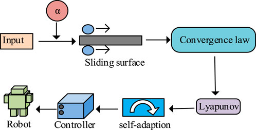
Figure 1. FOSMC application process.

As shown in Figure 1, the calculation process of FOSMC first defines and calculates fractional-order derivatives and introduces fractional-order differential operators. Within the sliding mode controller framework, the fractional-order sliding surface undergoes computation, while differential operators are employed to adjust the sliding reaching law. Finally, the adaptive law is calculated to complete the controller construction and control the robot. Fractional-order differential is a method of calculus extended to any order. By extending derivatives to arbitrary orders, non-integer order calculus can be obtained (Znidi et al., 2024). Fractional-order differentiation has multiple definitions, among which Caputo definition is efficient and convenient, showing good practical performance. The equation of Caputo definition is shown in Equation 1.

${}_{0}D_t^{\alpha }f\left(t\right)=\frac{1}{\mathrm{\Gamma }\left(n-\alpha \right)}{\displaystyle {\int }_0^t}\frac{f^{\left(n\right)}\left(\tau \right)}{{\left(t-\tau \right)}^{1-\left(n-a\right)}}d\tau (1)$

Equation 1: defines $\alpha$ as the upper limit of differentiation, representing the order of the derivative, which can take any real value. $t$ is the lower limit of differentiation, $\mathrm{\Gamma }\left(.\right)$ is the gamma function, $n$ is the current order, satisfying $n-1\le \alpha <n$, $n\in N$.

Introducing fractional-order calculus operators into the sliding surface calculation improves the stability of the sliding surface. A simple first-order fractional sliding surface equation is shown in Equation 2.

$D^{\alpha }x=-kx(2)$

Equation 2: $k$ is a constant and $k>0$. Its variation reflects the convergence efficiency of sliding surface motion.

In FOSMC, the sliding reaching law is adjusted through differential operators. The fractional-order sliding reaching law equation is shown in Equation 3.

$D^{\alpha }s=-ksgn\left(s\right)(3)$

Equation 3: $sgn\left(.\right)$ represents the sign function and $s$ represents the switching function.

In order to analyze the stability of the system, the Lyapunov function is derived. The definition formula of the Lyapunov function is shown in Equation 4.

$V\left(t\right)=1/2s^2(4)$

According to the Lyapunov function formula and the calculus operator, the derivation of the Lyapunov function is finally obtained as shown in Equation 5.

$\text{sgn}\left(V{\left(t\right)}^{\prime }\right)=\text{sgn}\left(s\right)\text{sgn}\left(D^{1-\alpha }{D}^{\alpha }s\right)=-k(5)$

Equation 5: $V{\left(t\right)}^{\prime }$ represents the derivative of the Lyapunov function combined with the reaching law and sliding surface calculation equation, $V{\left(t\right)}^{\prime }\le 0$, according to Lyapunov function stability theorem, fractional order sliding controller has good stability.

FOSMC has good stability and control performance but depends heavily on parameter tuning. PSO algorithm optimizes parameters by comparing individual extremes and global extremes. It can optimize controller parameters and help the controller adjust dynamically, improving performance (Butler et al., 2025). Therefore, PSO is used to optimize and improve the FOSMC structure. The optimization process is shown in Figure 2.

Figure 2

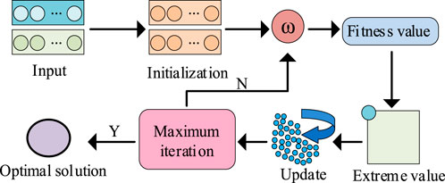
Figure 2. PSO algorithm optimization process.

In Figure 2, PSO first initializes related parameters and calculates inertia weight. The particle velocity and position are corrected according to the inertia weight. Individual and global extremes are continuously updated and compared to update the optimal solution. Upon attaining the maximum iteration threshold, the global extreme updated in the last iteration is output as the optimal solution. The update of individual particle extremes is mainly realized by correcting velocity and position. The particle velocity correction equation is shown in Equation 6.

$v_i\left(m+1\right)=v_i\left(m\right)+c_1\times \mathit{ran}{d}_1\times \left(p{b}_i\left(m\right)-x_i\left(m\right)\right)+c_2\times \mathit{ran}{d}_2\times \left(gb\left(m\right)-x_i\left(m\right)\right)(6)$

Equation 6: $m$ is the current iteration, $i$ represents a particle, $c_1$ and $c_2$ are the acceleration constants for the single particle and particle swarm, usually ranging from (0, 4). $v_i\left(m\right)$ is the particle $i$ velocity at iteration $m$. $p{b}_i\left(m\right)$ and $gb\left(m\right)$ are the individual and global extremes at iteration $m$.

The particle position in a certain iteration depends on the updated velocity and previous position. The particle position correction equation is shown in Equation 7.

$x_i\left(m+1\right)=x_i\left(m\right)+v_i\left(m+1\right)(7)$

Equation 7: $x_i\left(m\right)$ is the position of particle $i$ at iteration $m$. In PSO, the dynamic value of inertia weight balances the particle search range and convergence speed. The inertia weight update calculation is shown in Equation 8.

$w=w_{\max }-\frac{m}{m_{\mathit{max}}}\times \left(w_{\mathit{max}}-w_{\mathit{min}}\right)(8)$

Equation 8: $m_{\mathit{max}}$ is the maximum iteration number. The particle velocity correction equation after adjusting by inertia weight is shown in Equation 9.

$v_i{\left(m+1\right)}^{\prime }=w\times v_i\left(m+1\right)(9)$

Equation 9: $v_i\left(m+1\right)$ represents the velocity of particle $i$ at iteration $m+1$, and $w$ represents the inertia factor.

Through the equilibrium adjustment of inertia factors, particles continuously update their positions and gradually converge to the optimal solution. In the PSO algorithm, a fitness function is typically employed to evaluate the quality of each particle’s corresponding optimal solution, guiding the swarm toward global convergence. The definition formula for the fitness function is shown in Equation 10.

$fitness=1/\left(1+f\left(x\right)\right)(10)$

Equation 10: $f\left(x\right)$ represents the particle optimal solution.

The particle continuously updates its position and gradually converges to the optimal solution through balancing by the inertia factor. The PSO-based improved FOSMC enhances parameter optimization, but vibration suppression still needs improvement. RBFNN consists of output layer, hidden layer, and input layer. It can adjust sliding surface parameters and improve the vibration suppression of the sliding mode controller (Ece and Nizami, 2023). Therefore, RBFNN is combined with PSO to improve FOSMC, forming the PSO-RBF-FOSMC algorithm to enhance controller performance. The structure of PSO-RBF-FOSMC is shown in Figure 3.

Figure 3

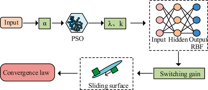
Figure 3. PSO-RBF-FOSMC structure.

As shown in Figure 3, the PSO-RBF-FOSMC algorithm consists of three core components: the RBF layer, FOSMC layer, and PSO layer. The process begins with calculating a fractional-order differential operator. This operator is then applied to compute the Sliding surface and its convergence law. In the PSO layer, the controller architecture undergoes training and optimization to identify optimal Sliding surface parameters that balance convergence speed with vibration suppression. These PSO-optimized parameters are fed into the RBF network using the least squares method as the adaptive rule, which adjusts the output layer weights. The RBF network subsequently performs online fitting to compensate for system uncertainties, dynamically adjusts switching gain to minimize high-frequency switching-induced vibrations, and ultimately achieves adaptive adjustments through the adaptive law.

3.2 Trajectory tracking control model based on PSO-RBF-FOSMC

The designed PSO-RBF-FOSMC controller improves vibration suppression and convergence speed. However, in actual robot operation, relying solely on the sliding mode controller cannot resist external influences and cannot complete normal work tasks. Robot kinematic modeling calculates the robot’s own structure. By computing parameters such as the velocity and position relationships of operating components, the robot’s components are analyzed and expressed to enable more precise control (Tuan et al., 2024). Therefore, this study conducts kinematic modeling based on the structure of the mobile robot. The kinematic modeling process is shown in Figure 4.

Figure 4

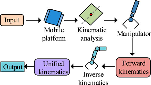
Figure 4. Kinematic modeling process of the robot.

As shown in Figure 4, the kinematic modeling process mainly includes mobile platform modeling and manipulator modeling. First, parameters such as the center of mass and radius of the mobile platform are measured, and the kinematic expressions of the mobile platform are calculated. Subsequently, the manipulator undergoes modeling processes, whereupon the relative pose between the end-effector and base is computed, with inverse solutions being derived through analysis of the end-effector’s relative positioning. Finally, the calculation equations of the mobile platform and manipulator are combined for unified kinematic modeling. The manipulator is the main operating component of the robot. Its kinematic modeling process includes forward kinematics and inverse kinematics. The study uses Denavit-Hartenberg (DH) parameters to accurately describe the relationship between manipulator joints and the end-effector for forward kinematics to obtain the end-effector position. Suppose there are $n+1$ coordinate frames numbered from $\left\{0\right\}$ to $\left\{n\right\}$, ${{}_i}^{i-1}T$ represents the homogeneous transformation matrix, and ${}^{i}P$ represents the position of the same point in $\left\{i\right\}$ frame. The position of the same point in $\left\{0\right\}$ frame using DH parameters is shown in Equation 11.

$oP{=}_1^0{T}_2^{1}T..{.}_n^{n-1}{T}^{n}P{,}^{0}p{=}_n^0{T}^{n}P(11)$

Equation 11: ${{}_n}^{n-1}T$ constitutes the homogeneous transformation matrix facilitating the conversion from frame $\left\{n-1\right\}$ to frame $\left\{n\right\}$, while ${}^{n}P$ denotes the positional coordinates of the identical point within the end-effector frame $\left\{n\right\}$.

Based on Equation 11, the forward kinematics equation of the manipulator is obtained in Equation 12.

${}_n{}^{0}T{=}_1^{0}1T_2^{1}T..{.}_n^{n-1}T(12)$

Equation 12: ${}_n{}^{0}T$ is the end-effector relative pose.

Drawing upon the end-effector pose established from forward kinematic calculations, inverse kinematics is calculated using the Newton-Raphson iteration method for solving complex nonlinear equations. First, the partial derivative of end-effector position $\left(x,y\right)$ with respect to joint angle ${\theta }_1$ is calculated, as shown in Equation 13.

$\left\{\begin{array}{l}\frac{\mathrm{\partial }x}{\mathrm{\partial }{\theta }_1}=-l_1\mathit{sin}\left({\theta }_1\right)-l_2\mathit{sin}\left({\theta }_1+{\theta }_2\right)-l_3\mathit{sin}\left({\theta }_1+{\theta }_2+{\theta }_3\right)\\ \frac{\mathrm{\partial }y}{\mathrm{\partial }{\theta }_1}=l_1\mathit{cos}\left({\theta }_1\right)+l_2\mathit{cos}\left({\theta }_1+{\theta }_2\right)+l_3\mathit{cos}\left({\theta }_1+{\theta }_2+{\theta }_3\right)\end{array}\right.(13)$

Equation 13: $l_1$, $l_2$, $l_3$ represent the link lengths. Based on Equation 11, the partial derivatives corresponding to end-effector position $\left(x,y\right)$ relative to joint angles ${\theta }_2,{\theta }_3$, $\frac{\mathrm{\partial }x}{\mathrm{\partial }{\theta }_2}$, $\frac{\mathrm{\partial }y}{\mathrm{\partial }{\theta }_2}$, $\frac{\mathrm{\partial }y}{\mathrm{\partial }{\theta }_2}$, $\frac{\mathrm{\partial }y}{\mathrm{\partial }{\theta }_3}$ are obtained.

These derivatives construct the Jacobian matrix $J$, and the updated joint angles are obtained according to Equation 14.

${\theta }_{new}={\theta }_{old}+\Delta \theta ,\Delta \theta =J^{+}·\left[\begin{array}{l}\Delta x\\ \Delta y\end{array}\right](14)$

Equation 14: $\Delta \theta ={\left[\Delta {\theta }_1,\Delta {\theta }_2,\Delta {\theta }_3\right]}^T$ represents the increment of joint angles, and $J^{+}$ represents the pseudoinverse of $J$.

To control the robot more precisely, dynamic analysis and modeling are conducted based on kinematic modeling. The dynamic modeling process is shown in Figure 5.

Figure 5

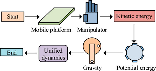
Figure 5. Dynamic modeling process of the robot.

As shown in Figure 5, dynamic modeling first calculates the kinetic and potential energy of the mobile platform and manipulator based on their kinematic modeling. Then, the total system kinetic and potential energy and gravity are calculated to complete unified dynamic modeling. To simplify derivation and improve generality, the study uses the Lagrange method for dynamic modeling. Lagrange method usually introduces generalized coordinates. Suppose there is a generalized coordinate $q={\left[q_1,q_2,...,q_n\right]}^T$, the calculation equation is shown in Equation 15.

$\frac{d}{dt}\left(\frac{\mathrm{\partial }L}{\mathrm{\partial }{\dot{q}}_i}\right)-\frac{\mathrm{\partial }L}{\mathrm{\partial }{q}_i}={\tau }_i,i=1,2,...,n(15)$

Equation 15: $q_i$ represents joint angle, ${\dot{q}}_i$ represents particle velocity, and ${\tau }_i$ represents joint torque or force.

The kinetic energy calculation is shown in Equation 16.

$T={\displaystyle \sum _{k=1}^n}\left(\frac{1}{2}{m}_k{v_k}^T{v}_k+\frac{1}{2}{{\omega }_k}^T{I}_k{\omega }_k\right)(16)$

Equation 16: $m_k$ represents the mass of the $k$-th link, $I_k$ represents the inertia tensor, and $v_k$ and ${\omega }_k$ represent translational and rotational velocities of the link.

The potential energy calculation is shown in Equation 17.

$V={\displaystyle \sum _{k=1}^n}{m}_{k}g{h}_k\left(q\right)(17)$

Equation 17: $h_k\left(q\right)$ is the vertical coordinate of the link’s center of mass, satisfying $g=9.8m/s$, and represents gravitational acceleration.

Based on kinetic and potential energy, the Lagrangian is calculated as shown in Equation 18.

$L=T-V(18)$

By organizing and deriving Equation 18, the dynamic equations of the system are obtained. Dynamic modeling using the Lagrange method enables more precise robot control. The improved PSO-RBF-FOSMC controller enhances system stability and control performance. Combining it with dynamic modeling improves system performance in multiple aspects. Therefore, to achieve more precise and stable trajectory tracking, the study raises a trajectory tracking control model based on improved FOSMC and dynamic modeling, named IFOSMC-DM-TTC. The overall process of the model is shown in Figure 6.

Figure 6

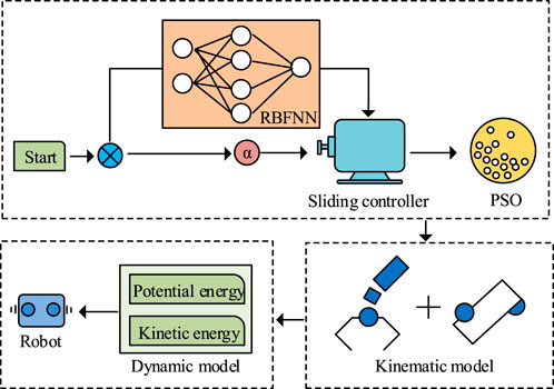
Figure 6. IFOSMC-DM-TTC trajectory control model process.

In Figure 6, the proposed PSO-RBF-FOSMC-based model mainly consists of FOSMC, kinematic modeling, and dynamic modeling. Initially, fractional-order differential operators undergo introduction into the sliding mode controller architecture for the purpose of determining the sliding surface and reaching law through computational processes. Then RBFNN adjusts the weights, followed by PSO optimizing the controller. The robot undergoes kinematic modeling of the mobile platform and manipulator based on the operating components. Finally, the Lagrangian is obtained from total kinetic and potential energy calculation for dynamic modeling, completing the robot trajectory tracking control.

4 Performance verification and analysis of robot trajectory tracking control model

4.1 Performance verification of improved controller based on PSO-RBF-FOSMC

To evaluate the performance of the PSO-RBF-FOSMC controller, this study conducted comparative validation using two control systems: the Nonlinear Disturbance Observer-Based Control (NDOBC) and the Fuzzy Proportion Integration Differentiation (Fuzzy PID). Through a stochastic search algorithm, we identified optimal parameter combinations by evaluating performance metrics across different configurations, ultimately determining the most effective parameters for the comparison algorithm. The experimental platform used Matlab software. The experimental object was a six-degree-of-freedom FVR6-6423 industrial robot, composed of a manipulator, conveyor belt, HD camera, and rotary cylinder. The camera was a web HD camera controlled by an industrial computer. The experiment was simulated by setting different parameters, as shown in Table 1.

Table 1

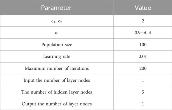
Table 1. Experimental parameter setting.

According to the above parameter setting, PSO-RBF-FOSMC controller is constructed for experiment. In order to verify the effectiveness of PSO and RBF algorithms in PSO-RBF-FOSMC controller, ablation experiments were set up. Taking FOSMC as the benchmark algorithm, the feedback error of the controller was compared and analyzed under three conditions: adding PSO algorithm only, adding RBF algorithm only, and adding PSO and RBF algorithm at the same time. The comparison results are shown in Figure 7.

Figure 7

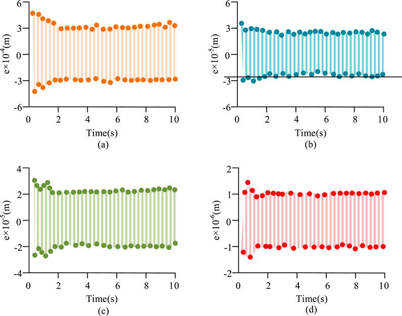
Figure 7. Shows the results of the ablation experiment. (a) The feedback error curve of FOSMC. (b) The feedback error curve of PSO-FOSMC. (c) The feedback error curve of RBF-FOSMC. (d) The feedback error curve of PSO-RBF- FOSMC.

As can be seen from Figure 7a, the oscillation range of the feedback error curve of the FOSMC controller in the stable state is [−3.0 × 10⁻⁴, 3.0 × 10⁻⁴]. It can be seen from Figures 7b,c that after adding the PSO algorithm for parameter tuning, the oscillation range of the controller feedback error curve in the stable state has decreased to [−2.7 × 10⁻⁵, 2.7 × 10⁻⁵]. After adding the RBF algorithm for parameter tuning, The oscillation range of the controller feedback error curve in a stable state has decreased to [−2.1 × 10⁻⁵, 2.1 × 10⁻⁵]. This result indicates that both the PSO algorithm and the RBF algorithm can effectively enhance the control performance of the model. As can be seen from Figure 7d, after the combination of the PSO algorithm and the RBF algorithm, the oscillation range of the controller in the stable state has decreased to [−1.1 × 10⁻⁵, 1.1 × 10⁻⁵], which is significantly lower than the feedback error after only adding the RBF algorithm and only adding the PSO algorithm. This further verifies the effectiveness of the PSO and RBF algorithms. It is also indicated that after the PSO-RBF-FOSMC controller is improved by combining the PSO algorithm and the RBF algorithm, the control performance has been significantly enhanced. To verify the control effect, the feedback errors of each algorithm were compared. The results are shown in Figure 8.

Figure 8

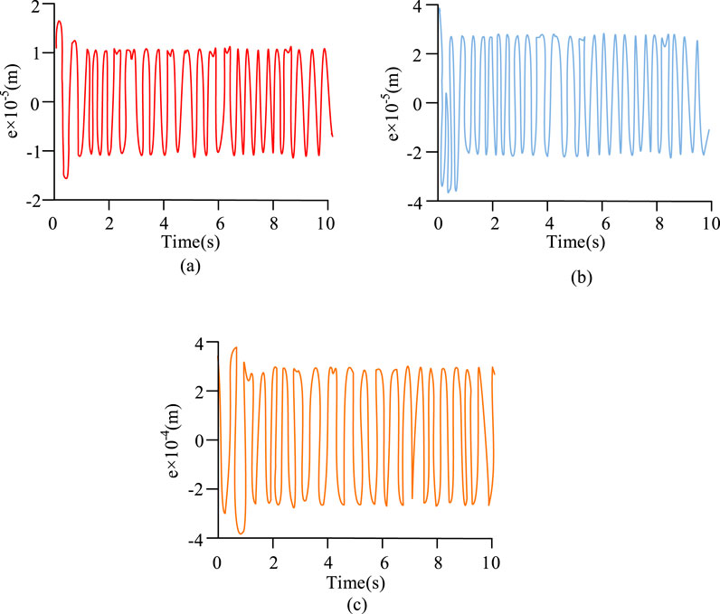
Figure 8. Feedback error graphs of each control algorithm. (a) The feedback error curve of PSO-RBF-FOSMC. (b) The feedback error curve of NDOBC. (c) The feedback error curve of NDOBC.

As shown in Figure 8, the error range of Fuzzy PID oscillated between [−2.3 × 10⁻⁴, 2.3 × 10⁻⁴], the largest among all algorithms, indicating a higher error deviation. In contrast, the feedback error of PSO-RBF-FOSMC remained within [−1 × 10^-5, 1 × 10⁻⁵], lower than other algorithms, showing higher accuracy. Furthermore, Fuzzy PID and NDOBC reached steady states around 0.6 s and 0.8 s, respectively, while PSO-RBF-FOSMC reached a steady state after 0.3 s. This indicated that PSO-RBF-FOSMC adapted more quickly and had faster adjustment speed. To further verify trajectory tracking, the position tracking trajectories of each algorithm were compared. The results are shown in Figure 9.

Figure 9

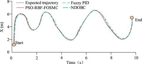
Figure 9. Position tracking curves of different algorithms.

Figure 9 shows that Fuzzy PID completed adaptive adjustment after 0.8 s, which was slower. PSO-RBF-FOSMC completed adaptive adjustment after 0.3 s, indicating faster convergence. Moreover, the position tracking trajectory of Fuzzy PID after adjustment still deviated noticeably from the desired trajectory, while the trajectory of PSO-RBF-FOSMC coincided with the desired trajectory much better, demonstrating higher accuracy. For further performance analysis, the tracking speed along the X-axis was calculated and compared, as shown in Figure 10.

Figure 10

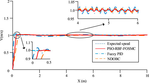
Figure 10. Tracking speed comparison along X-axis.

Figure 10 shows that the speed curve of PSO-RBF-FOSMC coincided with the desired speed more closely than other algorithms, showing better control. The left zoomed view indicated that the PSO-RBF-FOSMC control speed along the X-axis nearly matched the desired speed at around 0.25 s, stabilizing at 1 m/s, showing fast convergence and high precision. The right zoomed view shows that the PSO-RBF-FOSMC speed curve was the closest to the desired speed, smooth, and with minimal deviation. In summary, PSO-RBF-FOSMC demonstrated superior stability and convergence speed compared to the other algorithms.

4.2 Analysis of practical application effect of trajectory tracking control model

Based on the performance analysis of PSO-RBF-FOSMC, the proposed IFOSMC-DM-TTC trajectory tracking control model was evaluated. The same experimental environment was used, and Sparrow Search Algorithm-PID (SSA-PID), Adaptive Untraceable Kalman Filter-Nonlinear Model Predictive Control (AUKF-NMPC), and Model Predictive Control-Sliding Mode Control (MPC-SMC) were selected for comparison. In order to ensure the fairness of the experiment and the reliability of the results, the parameters of each model are adjusted to the best practice parameters to ensure that each model is in the optimal working state. To ensure experimental fairness and result reliability, all model parameters were adjusted to best practice levels to maintain optimal operational states. For robustness verification, the study generated 5 m/s gust wind using variable-frequency fans, creating a wind interference scenario. The robot traveled along a continuous path from tile floor to carpet to sandy ground, simulating abrupt friction changes across surfaces. Each surface segment (tile, carpet, sand) measured 5 m in length. Sensor noise interference was introduced by injecting Gaussian white noise, while a 300g mass block was attached to the robotic arm’s end for load testing. Comparative analysis of lateral root mean square errors across scenarios yielded results shown in Table 2.

Table 2

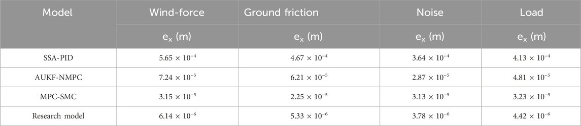
Table 2. Comparison of experimental error in robustness test.

As shown in Table 1, the proposed IFOSMC-DM-TTC model demonstrates the lowest lateral error of 6.14 × 10^-6 m in wind interference scenarios, showing superior accuracy compared to benchmark algorithms. In ground friction abrupt change scenarios, the model achieves a lateral error of 5.33 × 10^-6 m, significantly lower than competing models and demonstrating enhanced stability. Under noise interference and load interference conditions, the model’s lateral errors measure 3.78 × 10^-6 m and 4.42 × 10^-6 m respectively, both outperforming comparison models. This indicates the model’s robust adaptability across diverse scenarios. Overall, the proposed model maintains minimal errors across various interference conditions while exhibiting strong anti-interference capabilities. To further verify performance, the rise time and overshoot of each model were calculated and compared, as shown in Figure 11.

Figure 11

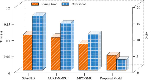
Figure 11. Rise time and overshoot comparison.

Figure 11 shows that IFOSMC-DM-TTC had a rise time of 0.06 s, 0.015 s faster than the fastest comparison model, MPC-SMC, indicating faster stabilization and better control. The overshoot of IFOSMC-DM-TTC was 5%, significantly lower than the comparison models, demonstrating effective vibration suppression. Overall, the proposed model combined rapid response, stability, and strong anti-disturbance ability. To evaluate application performance, the X-axis tracking speed of each model was calculated and analyzed, as shown in Figure 12.

Figure 12

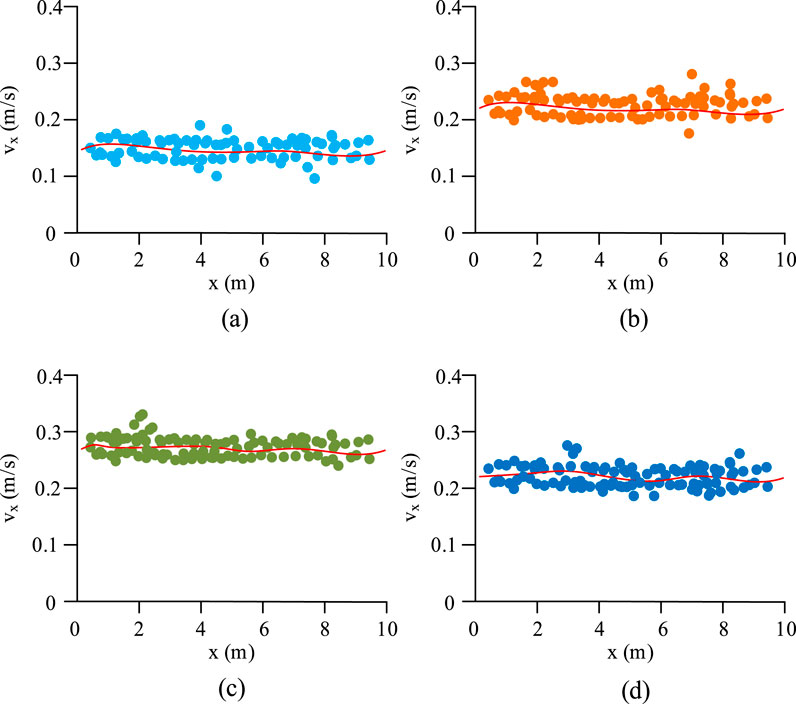
Figure 12. Tracking speed comparison along X-axis. (a) The velocity in the X-axis direction of SSA-PID. (b) The velocity in the X-axis direction of AUKF-NMPC. (c) The velocity in the X-axis direction of proposed model. (d) The velocity in the X-axis direction of MPC-SMC.

Figure 12c shows that IFOSMC-DM-TTC achieved an average X-axis tracking speed of 0.26 m/s, with uniform speed distribution and smooth trend, showing good vibration resistance. Overall, IFOSMC-DM-TTC exhibited significantly faster X-axis tracking speed than other models, indicating better control. In conclusion, IFOSMC-DM-TTC outperformed other models in speed, stability, and accuracy, demonstrating superior control performance and supporting efficient and safe robot operation.

5 Summary

This study addressed the issues of vibration sensitivity and high uncertainty in mobile robot trajectory tracking by constructing a trajectory tracking control model based on the PSO-RBF-FOSMC algorithm and dynamic modeling to improve robot control capability. The trajectory tracking controller was designed based on FOSMC and optimized using PSO and RBFNN. Then, kinematic modeling analysis and dynamic modeling were applied to the robot’s main operating components to enhance the accuracy of reference tracking control. To evaluate the performance of the reference tracking control model, simulation experiments were conducted to analyze its practical application. In the experiments, the position error of the PSO-RBF-FOSMC algorithm remained stable within the range of [−1 × 10^-5, 1 × 10⁻⁵], lower than the comparison algorithms. The control speed along the X-axis nearly coincided with the desired speed curve at around 0.25 s, demonstrating high precision. The proposed trajectory tracking control model achieved an X-axis tracking speed of 0.26 m/s, with a smooth speed trend curve and good vibration suppression. The rise time of the proposed model was 0.06 s, faster than the comparison models, indicating rapid convergence. These results showed that the proposed trajectory tracking control model achieved good performance in terms of accuracy, stability, and rise speed. Although the proposed model demonstrated strong control performance, it still exhibited some deviation from the desired trajectory, and the dynamic adjustment effect of the model was not analyzed. In the future, the accuracy and adaptive dynamic adjustment capability of the model will be analyzed and improved to enhance its practical application performance.

Data availability statement

The original contributions presented in the study are included in the article/supplementary material, further inquiries can be directed to the corresponding author.

Author contributions

NN: Conceptualization, Data curation, Formal Analysis, Investigation, Methodology, Writing – original draft, Writing – review and editing.

Funding

The author(s) declare that no financial support was received for the research and/or publication of this article.

Conflict of interest

The author declares that the research was conducted in the absence of any commercial or financial relationships that could be construed as a potential conflict of interest.

Generative AI statement

The author(s) declare that no Generative AI was used in the creation of this manuscript.

Any alternative text (alt text) provided alongside figures in this article has been generated by Frontiers with the support of artificial intelligence and reasonable efforts have been made to ensure accuracy, including review by the authors wherever possible. If you identify any issues, please contact us.

Publisher’s note

All claims expressed in this article are solely those of the authors and do not necessarily represent those of their affiliated organizations, or those of the publisher, the editors and the reviewers. Any product that may be evaluated in this article, or claim that may be made by its manufacturer, is not guaranteed or endorsed by the publisher.

References

Benzaouia, M., Benzaouia, S., Rabhi, A., Hajji, B., and Elgharib, A. O. (2024). Direct-driven PMSG wind turbines: adaptive super twisting algorithm Control approach. IFAC-PapersOnLine 58 (13), 757–762. doi:10.1016/j.ifacol.2024.07.573

CrossRef Full Text | Google Scholar

Bhat, A., Rao, V. S., and Jayalakshmi, N. S. (2025). Dynamic modeling of magnetorheological damper based three-link model for human lower limb. Int. J. Control 23 (3), 840–851. doi:10.1007/s12555-024-0323-4

CrossRef Full Text | Google Scholar

Butler, A. G., Bassi, J. K., Connelly, A. A., Melo, M. R., Allen, A. M., and Mcdougall, S. J. (2025). Vagal nerve stimulation dynamically alters anxiety-like behavior in rats. Brain Stimul. 18 (2), 158–170. doi:10.1016/j.brs.2025.01.018

PubMed Abstract | CrossRef Full Text | Google Scholar

Chen, A. N., Zhou, J., and Wang, K. (2024). Adaptive state-constrained/model-free iterative sliding mode control for aerial robot trajectory tracking. Appl. Math. Mech. Ed. 45 (4), 603–618. doi:10.1007/s10483-024-3103-8

CrossRef Full Text | Google Scholar

Demir, S., and Sahin, E. K. (2023). Predicting occurrence of liquefaction-induced lateral spreading using gradient boosting algorithms integrated with particle swarm optimization: pso-xgboost, PSO-LightGBM, and PSO-CatBoost. Acta Geotech. 18 (6), 3403–3419. doi:10.1007/s11440-022-01777-1

CrossRef Full Text | Google Scholar

Ece, Y., and Nizami, A. (2023). Dynamic modeling and nonlinear free vibration analysis of a rotating 3D beam induced by adjacent two revolute joints. Multibody Syst. Dyn. 59 (4), 429–446. doi:10.1007/s11044-023-09891-y

CrossRef Full Text | Google Scholar

Huang, H., Tang, G., Chen, H., Wang, J., Han, L., and Xie, D. (2025). Full-order sliding mode control of underwater flexible manipulators with echo state network disturbance compensation. Trans. Can. Soc. Mech. Eng. 49 (2), 249–263. doi:10.1139/tcsme-2023-0209

CrossRef Full Text | Google Scholar

Hamad, S. A., Xu, W., Junejo, A. K., Xiao, H., Tang, Y., Ghalib, M. A., et al. (2025). Improved full-order sliding mode based on model predictive flux control for LIM applied to urban transit. IEEE Trans. Transp. Electrification 11 (1), 2556–2570. doi:10.1109/tte.2024.3424496

CrossRef Full Text | Google Scholar

Kolahi, M. R. S., Moeinkhah, H., Rahmani, H., and Mohammadzadeh, A. (2024). Dynamic modeling and multi-objective optimization of a 3DOF reconfigurable parallel robot. Mech. Solids 59 (3), 1689–1706. doi:10.1134/s0025654424603483

CrossRef Full Text | Google Scholar

Luan, S., Sun, Y., Gong, L., and Zhang, K. (2024). Trajectory tracking method of agricultural machinery MultiRobot Formation operation based on MPC delay compensator. Smart Agric. 6 (3), 69–81. doi:10.12133/j.smartag.SA202306013

CrossRef Full Text | Google Scholar

Moran-Armenta, M., Aguilar-Avelar, C., Gandarilla, I., Meza-Sánchez, M., and Moreno-Valenzuela, J. (2025). Solving trajectory tracking of robot manipulators via PID control with neural network compensation. Soft Comput. 29 (2), 1227–1241. doi:10.1007/s00500-025-10439-9

CrossRef Full Text | Google Scholar

Ruqiang, M., and Le, L. (2024). Research on design and trajectory tracking control of a variable size lower limb exoskeleton rehabilitation robot. J. Mech. Sci. Technol. 38 (1), 389–400. doi:10.1007/s12206-023-1232-9

CrossRef Full Text | Google Scholar

Sandoval, J., Cervantes-Perez, L., Santibanez, J. K. R., Moreno-Valenzuela, J., and Kelly, R. (2024). A GES joint position trajectory tracking smooth controller of torque-driven robot manipulators affected by disturbances. Int. J. Robust Nonlinear Control 34 (2), 1032–1053. doi:10.1002/rnc.7015

CrossRef Full Text | Google Scholar

Tuan, N. T., Tien, V. H., and Van Minh, D. (2024). Synthesis of parameter Recognition Algorithm and State evaluation for separating target. Archives Adv. Eng. Sci. 2 (2), 100–107. doi:10.47852/bonviewaaes32021333

CrossRef Full Text | Google Scholar

Wang, G., Xie, C., Liu, C., and Cheng, J. (2024). Dynamic modeling of a hypersonic vehicle with structure, aerodynamic and propulsion coupling. Acta Aerodyn. Sin. 42 (10), 19–29. doi:10.7638/kqdlxxb-2023.0180

CrossRef Full Text | Google Scholar

Yunlong, Y., Xiaocheng, B., Guangen, H. Z., Zhang, H., and Zhou, G. (2024). Dynamic modeling and crawling gait control of six-strut spherical tensegrity robot. Adv. Robotics Int. J. Robotics Soc. Jpn. 38 (5), 323–342. doi:10.1080/01691864.2024.2321177

CrossRef Full Text | Google Scholar

Zhang, Q., Jiang, Y., Guo, G., and Zhang, Y. (2024). Finite time trajectory tracking control for partial actuator failure of underwater salvage robot. Chin. J. Ship Res. 19 (5), 57–64. doi:10.19693/j.issn.1673-3185.03430

CrossRef Full Text | Google Scholar

Zhu, W., and Wang, L. (2024). Adaptive finite-time fault-tolerant control for Robot trajectory tracking systems under a novel smooth event-triggered mechanism. J. Syst. Control Eng. 238 (2), 288–303. doi:10.1177/09596518231188495

CrossRef Full Text | Google Scholar

Zhu, M., Cao, Y., He, Z., Wu, Q., Ma, J., Qiu, B., et al. (2024). Research on fractional-order sliding mode PMSM speed regulation based on load observer. J. Electr. Eng. and Technol. 19 (5), 3429–3438. doi:10.1007/s42835-023-01661-2

CrossRef Full Text | Google Scholar

Znidi, A., Khlif, R. J., Nouri, S. D. N., and Derbel, N. (2024). Discrete second order sliding mode control for fractional order hammerstein System. ifac Pap. 58 (12), 347–352. doi:10.1016/j.ifacol.2024.08.214

CrossRef Full Text | Google Scholar