Fault diagnosis method for HVAC sensors based on improved 1-D CNN model and wavelet clustering analysis

Introduction: Heating, Ventilation and Air Conditioning (HVAC) sensor fault diagnosis is essential for ensuring the reliability and energy efficiency of intelligent building systems. However, existing diagnostic methods suffer from insufficient adaptability to multi-scale features, weak temporal dependency modeling, and poor generalization under small samples, and are highly sensitive to Gaussian noise.

Method: To address these limitations, this study proposes a fault diagnosis method that integrates an improved one-dimensional convolutional neural network (1-D CNN) with wavelet packet clustering. First, a multi-scale convolution module is designed using parallel 3/5/7 convolution kernels and residual connections to extract temporal features across different receptive fields. Then, wavelet packet decomposition is used to divide the original signal into eight frequency bands and construct energy feature vectors. K-means clustering is performed in an unsupervised manner, and Softmax-based weight fusion is used to realize end-to-end diagnosis with low computational overhead.

Results: Experimental results show that the proposed method achieves a diagnostic accuracy of 97.84% and an F1-score of 0.97. Under 30% Gaussian white noise, the area under the curve decreases by only 4%, and the instantaneous robustness drop increases by 0.01 within the 10%-30% noise range, demonstrating strong noise resistance and generalized learning capability.

Discussion and Conclusion: The proposed method effectively balances feature-scale adaptability, temporal modeling, and robustness under noisy and small-sample conditions. With low inference complexity and high diagnostic stability, it provides a feasible paradigm for real-time fault detection and reliable operation and maintenance in intelligent building HVAC systems.

1 Introduction

Heating, Ventilation and Air Conditioning (HVAC) systems exert a crucial role in modern buildings. It regulates the temperature, humidity, and air quality of indoor environments, which directly affects energy consumption, comfort, and equipment stability (Abrazeh et al., 2022; Huang and Liao, 2022). With the widespread application of smart buildings, the operational efficiency and reliability of HVAC systems are increasingly valued. As the core sensor of HVAC system, its accuracy and reliability directly determine the normal operation (Sousan et al., 2022). However, with prolonged use, sensors may malfunction, leading to abnormal data and ultimately affecting the overall efficiency. Timely diagnosing sensor faults is significant for the normal operation of HVAC systems. Al-Aomar et al. developed a joint predictive maintenance method that integrated building management system data and computerized maintenance management data to deal with the lack of real-time data-driven fault prediction for air handling units in hospital HVAC. This method combined support vector machine, decision tree, proximity algorithm, predictive prediction, and seasonal autoregressive integrated moving average model to achieve accurate fault prediction and effectively reduce maintenance costs (Al-Aomar et al., 2024). Patil et al. systematically reviewed HVAC fault characterization, classification, detection, and diagnosis to address the difficulty of identifying multi-source faults in HVAC and electrical systems. They proposed an intelligent monitoring and pre-maintenance strategy (Patil and Malwatkar, 2024). Wang et al. built an FDD relying on optimized Transformer-dual-decoder and adapter-based parameter efficient transfer learning to address the poor generalization of Fault Detection and Diagnosis (FDD) models in HVAC systems due to their diversity and high data acquisition costs. It migrated the source domain model to the new system with only a small amount of target domain data (Wang et al., 2024).

Deep learning has achieved significant progress in various fields, especially in fault diagnosis and prediction. Convolutional Neural Network (CNN) has achieved excellent results in image processing and speech recognition (Song et al., 2022). Zhao Z and Jiao Y proposed a hybrid information CNN architecture to solve the information loss caused by downsampling in rotating machinery fault diagnosis. The deep convolution was utilized to enhance the discriminative ability of spatial position. Traditional convolution achieved cross-channel interaction of information, thereby reducing the information loss of convolutional layers (Zhao and Jiao, 2022). Zhang Q and Deng L proposed a rolling bearing fault diagnosis method that combined Short-Time Fourier Transform (STFT) with CNN to solve the weak features when CNN directly processed raw vibration signals. STFT converted One-Dimensional (1D) vibration signals into time-frequency maps and inputted them into a two-layer CNN, improving the model fault diagnosis efficiency (Zhang and Deng, 2023). To solve the poor feature extraction accuracy in traditional HVAC chillers, Yan K and Zhou X proposed a CNN integrated feature extraction classification framework, which achieved FDD of chillers without feature engineering (Yan and Zhou, 2022). Iqbal M and Madan A K proposed an intelligent fault diagnosis method relying on vibration to detect bearing faults. CNN was taken to diagnose faults in CNC machine tools and STFT was utilized to convert raw signals like vibration and acoustic signals into time-frequency, achieving 100% accuracy (Iqbal and Madan, 2022).

In summary, although existing research on HVAC system fault diagnosis has achieved certain results, there are still problems such as insufficient model generalization ability, low feature extraction accuracy, and low efficiency of multi-source signal fusion. Although CNN performs well in fault feature extraction, it originates from the image field and is difficult to effectively model temporal dependencies. It is also not robust enough to feature scale changes, with multiple parameters and complex training, which limits its application in sensor fault diagnosis. Therefore, the study proposes to improve the 1-D CNN and introduces wavelet clustering analysis to construct a sensor fault diagnosis method, aiming to demonstrating theoretical and technical support for the efficient maintenance and safe operation of HVAC systems in intelligent buildings.

The innovation of this study lies in the deep integration of multi-scale time–frequency feature modeling and diagnostic strategies, which overcomes the limitations of traditional CNN-based or wavelet hybrid models. First, in the time-domain modeling stage, a Multi-Scale Convolution Module (MSCM) and residual connection structure are introduced, enabling the framework to simultaneously capture short-term local features and long-term global features within a single model, thereby achieving adaptive representation of fault signals at different temporal scales. Second, in the frequency-domain analysis stage, Wavelet Packet Transform (WPT) is employed to perform fine-grained signal decomposition and energy vector construction, offering higher frequency resolution compared to traditional wavelet transform that only decomposes the low-frequency components. Finally, in the decision-making mechanism, the fusion of Softmax outputs and clustering labels breaks the limitation of single time-domain decision-making in existing CNN models, enhances noise resistance and generalization capability, and achieves high-accuracy fault identification through time–frequency integration with unsupervised assistance.

2 Methods and materials

Firstly, an improved network is proposed that integrates MSCM, residual connections, and Class-Weighted Cross-Entropy (CWCE) loss function. Secondly, to explore the discriminative information of fault signals in the frequency domain, WPT is introduced to decompose the original sequence into eight refined frequency bands and construct normalized energy vectors. Subsequently, K-means unsupervised clustering is used to obtain frequency domain structural labels, thereby forming a robust diagnostic framework that is end-to-end and complementary in time-frequency.

2.1 Improved 1-D CNN model

CNN, as a typical deep learning structure, has been extensively applied in image recognition, speech processing, and fault diagnosis. To process 1D temporal signals, 1-D CNN has become one of the mainstream methods for sensor fault identification in HVAC systems due to its lightweight structure and high computational efficiency. Its structure is shown in Figure 1.

Figure 1

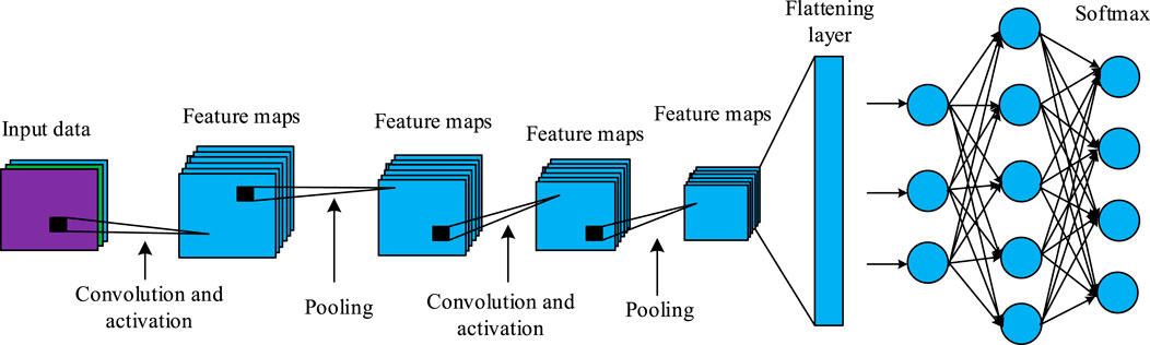
Figure 1. The traditional 1-D CNN.

In Figure 1, the traditional 1-D CNN mainly has an input layer, a convolutional layer, a pooling layer, a fully connected layer, and an output layer. In the feature extraction process, 1-D CNN first extracts local temporal features through convolutional layers, compresses dimensions through pooling layers, and inputs them into fully connected networks for classification (Groumpos, 2023; Ahmadzadeh et al., 2025). Although 1-D CNN has advantages such as high efficiency and simple structure in processing temporal signals, its convolutional kernel scale is fixed and cannot effectively extract multi-scale features, resulting in poor performance in dealing with fault signals of different frequencies or durations. As the depth of the network increases, 1-D CNN is prone to gradient vanishing or degradation, leading to unstable training. In addition, traditional structures lack the ability to jointly model low-level local features and high-level abstract features, which affects the comprehensiveness and refinement of fault pattern recognition. The research proposes an improved 1-D CNN model (Multi-Scale Residual 1-D CNN, MSR-1DCNN) depending on MSCM and residual connection mechanism. Firstly, MSCM is introduced to enhance the perception ability of different scale features in the model (Gao et al., 2022). The input sequence is $X\in {\mathbb{R}}^L$. $L$ represents the length of the input signal and the data comes from various HVAC sensors like temperature, humidity, and pressure. Therefore, the feature map corresponding to the $i$-th convolution kernel $W_i$ is shown in Equation 1.

$\begin{array}{cc}{F}_i=\text{ReLU}\left(\text{BN}\left(W_i*X+b_i\right)\right),& i\in \left\{1,2,3\right\}\end{array}(1)$

In Equation 1, $F_i$ signifies the feature map. $\text{ReLU}$ signifies the activation function of the linear rectification unit, used to enhance nonlinear modeling capabilities. $\text{BN}$ represents batch normalization operation. $b_i$ represents the bias term. $*$ represents 1D convolution operation. Three sets of convolution kernels ($k_1$ = 3, $k_2$ = 5, and $k_3$ = 7) are introduced for feature extraction, extracting potential abnormal behavior features from those exceeding the local, intermediate, and global scales, respectively, to avoid single scale models ignoring certain types of faults (Niu et al., 2021). After MSCM output, the features of the three channels are concatenated to form a unified representation, as shown in Equation 2.

$F_{\text{multi}}=\text{Concat}\left(F_1,F_2,F_3\right)(2)$

In Equation 2, $F_{\text{multi}}$ represents the concatenated multi-scale feature combination. $\text{Concat}$ represents merging multiple feature maps along the channel direction to form a joint feature representation. To maintain the underlying information of the original input and the stability of gradient propagation, a residual jump connection mechanism is introduced, as shown in Equation 3.

$F_{\text{res}}=F_{\text{multi}}+\mathbb{Q}\left(X\right)(3)$

In Equation 3, $F_{\text{res}}$ represents the feature representation after residual fusion. $\mathbb{Q}\left(X\right)$ represents the mapping function after dimension matching for input $X$, using identity mapping. The feature $F_{\text{res}}$ after residual fusion is unfolded through Flatten layers, input into a two-layer fully connected network, and connected to Softmax for output. The specific mathematical expression is shown in Equation 4.

$\begin{array}{cc}{\widehat{y}}_k=\frac{\exp \left(z_k\right)}{{\displaystyle {\sum }_{j=1}^C}\exp \left(z_k\right)},& k=1,2,...,C\end{array}(4)$

In Equation 4, ${\widehat{y}}_k$ signifies the prediction probability of the $k$-class fault. $z_k$ signifies the score value of the $k$-th output neuron. $C$ signifies the total fault classes. $\exp \left(·\right)$ represents an exponential function, primarily responsible for normalizing the output to probability (Qiu et al., 2023). Considering the class imbalance in actual fault data, this study adopts CWCE to enhance the model’s classification fairness and small sample fault recognition ability (Arkin et al., 2023), as shown in Equation 5.

$Loss=-{\displaystyle \sum _{k=1}^C}{w}_k·y_k\log \left({\widehat{y}}_k\right)(5)$

In Equation 5, $Loss$ represents the overall loss function value. $y_k$ represents the $k$-th dimension of the true label, with a value of 0 or 1. $w_k$ represents the class weight coefficient, defined as $w_k=\frac{1}{N_k}$. $N_k$ signifies the quantity of samples in the $k$-th class to avoid training bias caused by imbalanced categories. Based on the above, the proposed MSR-1DCNN structure is shown in Figure 2.

Figure 2

Figure 2. Improved MSR-1DCNN structure.

In Figure 2, the study first introduces a MSCM, which parallelly configures convolution layers with different receptive fields to enable the model to simultaneously model short-term fluctuations and long-term trends, thereby effectively improving the ability to extract multiple fault features. Secondly, the residual connection mechanism introduces an identity mapping path of input information in the convolution module, enhancing the trainability of deep networks, alleviating gradient vanishing, and synergistically modeling shallow and deep features. Normalization and regularization mechanisms are introduced, and Batch Normalization and Dropout layers are added after each convolution unit to optimize the convergence speed and generalization performance and suppress overfitting. In addition, the output layer adopts the Softmax function and combines it with the CWCE strategy to enable the model to still have good fault discrimination ability in scenarios with imbalanced sample sizes. Overall, the MSR-1DCNN structure optimizes the recognition accuracy and robustness in complex working conditions and diverse fault types by constructing a learning framework that integrates multi-scale, multi-path, and deep shallow features.

2.2 Design of fault diagnosis method

On the basis of completing multi-scale feature extraction and deep feature fusion in the improved MSR-1DCNN model, the wavelet clustering analysis mechanism is introduced to achieve high-precision discrimination and automatic classification of fault modes. This method employs the multi-resolution characteristics of WPT, which can unfold complex temporal signals in different frequency bands and quantify their energy distribution characteristics. To ensure the accuracy of time-frequency decomposition and the stability of feature extraction, the study selected db4 from the Daubechies wavelet family as the basis function in the WPT decomposition and set a three-layer decomposition depth to obtain eight frequency band energy features. The db4 wavelet has good time-frequency localization and smoothness in the field of signal analysis and is suitable for typical HVAC sensor signal characteristics such as non-stationary and transient disturbances (Huang et al., 2024). The determination of the number of decomposition layers comprehensively considers the sampling frequency, the main frequency band distribution, and the coverage of the characteristic frequency: on the one hand, the power spectrum estimation shows that the signal is mainly concentrated in the low to medium frequency band; on the other hand, although too deep decomposition can improve the resolution, it will cause energy dispersion and increase the computational burden (Moumene and Ouelaa, 2022). Therefore, the signal is divided into eight equal-width sub-bands, which not only ensures the frequency resolution but also facilitates the fault feature identification. WPT decomposes signal $f\left(t\right)$ in the $J$-layer to obtain $2^J$ sub-signals $U_j\left(t\right)$ in different frequency bands, each corresponding to specific frequency range information. Figure 3 presents the specific structure.

Figure 3

Figure 3. Three-layer WPT structure.

In Figure 3, the original signal is first decomposed into low-frequency sub-bands (Approximation) and high-frequency sub-bands (Detail), and then each sub-band continues the same binary decomposition in the next layer until it realizes the set three-layer depth. After three layers of decomposition, the signal is divided into 2³ sub-nodes in different frequency bands, representing the energy distribution from the lowest frequency band to the highest frequency band. Each node corresponds to a sub-signal within a fixed frequency range. By calculating the energy of each node, it can comprehensively reflect the changing trend of the original signal in different frequency domains. This structure can capture the spectral changes caused by sensor faults in detail, providing high-resolution frequency domain feature support for subsequent energy vector construction and clustering analysis. Compared to traditional wavelet decomposition that only iterates on the low-frequency part, WPT has stronger frequency resolution and is suitable for processing non-stationary and nonlinear fault signals in HVAC systems. Based on the transformation results, extracting the energy features of each frequency band is expressed as Equation 6.

$\begin{array}{cc}{E}_j={\displaystyle \sum _{m=1}^M}{\left|U_j\left(m\right)\right|}^2,& j=1,2,...,\end{array}{2}^J(6)$

In Equation 6, $E_j$ signifies the energy of the $j$-th wavelet packet frequency band. $U_j\left(m\right)$ signifies the amplitude coefficient of the $j$-th frequency band at the $m$-th time. $M$ represents the total samples in each frequency band. To eliminate the influence of signal amplitude and sampling duration on energy indicators, energy normalization is used to construct a normalized energy vector. The specific mathematical expression is shown in Equation 7.

$\begin{array}{cc}\mathbf{E}=\left[\frac{E_1}{E_T},\frac{E_2}{E_T},...,\frac{E_{2^J}}{E_T}\right],& E_T={\displaystyle \sum _{j=1}^{2^J}}{E}_j\end{array}(7)$

In Equation 7, $\mathbf{E}\in {\mathbb{R}}^{2^J}$ represents the normalized energy feature vector as the frequency domain expression for each segment of the signal. $E_T$ represents the total energy, with a standardized denominator. $\frac{E_j}{E_T}$ represents the energy proportion of frequency band $j$. After obtaining the energy features of all samples, the K-means clusters and analyzes the energy vectors to discover the inherent differences in frequency energy distribution of different signals and assist in distinguishing fault modes. The optimization objective of K-means is to minimize the sum of squared distances from a sample to its cluster center, as presented in Equation 8.

$\underset{G,\mu }{\min }{{\displaystyle \sum _{k=1}^K}{\displaystyle \sum _{{\mathbf{E}}^{\left(i\right)}\in G_k}}‖{\mathbf{E}}^{\left(i\right)}-{\mu }_k‖}^2(8)$

In Equation 8, $G_k$ represents the $k$-th cluster. $K$ represents the number of clusters, determined by the actual fault type or selected through contour coefficients. ${\mathbf{E}}^{\left(i\right)}$ signifies the energy feature vector of the $i$-th sample. ${\mu }_k$ signifies the center vector of class $k$. $‖·‖$ represents the Euclidean distance function. Based on the above equation, structural classification of different fault signals can be completed without relying on tag information. However, relying solely on clustering results for fault identification still has certain limitations, such as sensitivity to noise and strong dependence on initial clustering centers. Therefore, the probability distribution output by the improved MSR-1DCNN model is further fused with wavelet clustering label information to construct a fusion discrimination mechanism, which enhances the stability and accuracy of the final diagnosis. Assuming that the $i$-th sample is calculated by the MSR-1DCNN model, the Softmax output is ${\widehat{y}}_c^{\left(i\right)}$, where $c=1,2,...,C$ is the fault class number. Meanwhile, the sample is subjected to wavelet energy vector ${\mathbf{E}}^{\left(i\right)}$ to calculate the clustering label $c_{\text{cluster}}^{\left(i\right)}$. The final fusion discrimination result can be determined by Equation 9.

$y^{\left(i\right)}=\underset{c}{\mathrm{argmax}}\left(\alpha ·{\widehat{y}}_c^{\left(i\right)}+\left(1-\alpha \right)·\delta \left(c,c_{\text{cluster}}^{\left(i\right)}\right)\right)(9)$

In Equation 9, $y^{\left(i\right)}$ represents the final identified fault class label. ${\widehat{y}}_c^{\left(i\right)}$ represents the prediction probability that sample $i$ belongs to class $c$ by MSR-1DCNN. $c_{\text{cluster}}^{\left(i\right)}$ represents the analysis result of K-means clustering. $\alpha$ represents the fusion weight factor, mainly used to control the proportion of the impact of two types of information on the final output. $\delta \left(c,c_{\text{cluster}}^{\left(i\right)}\right)$ represents an exponential function used to determine whether categories $c$ and $c_{\text{cluster}}^{\left(i\right)}$ are equal and return a Boolean result (equal is 1, and unequal is 0). In the fusion discrimination mechanism, the Softmax output reflects the confidence of time-domain features, while the WPT cluster labels characterize the energy structure in the frequency domain. By setting the fusion weight, the two are linearly weighted: when the results are consistent, the confidence is enhanced, and when they are inconsistent, complementary corrections are made, thereby improving the stability and robustness of the classification. Based on the above, the HVAC sensor fault diagnosis process using the improved MSR-1DCNN model and WPT is shown in Figure 4.

Figure 4

Figure 4. HVAC sensor fault diagnosis process based on MSR-1DCNN and wavelet cluster analysis.

In Figure 4, time-series data from multiple sensor channels are input into the MSR-1DCNN model. After multi-scale convolution, residual connection, and normalization, high-dimensional and deep time-domain feature representations are extracted, and the corresponding Softmax fault probability distribution is output. The original signal is synchronously input into the WPT module, which performs multi-layer decomposition to extract energy features of each frequency band and construct energy vectors. Softmax outputs are trained through supervised training based on time-domain features, providing classification probabilities. K-means clustering, based on frequency-domain energy distribution, can identify spectral structural patterns without labels. By setting weights, confidence is enhanced when the two results are consistent, while clustering information is used to correct the predicted distribution when they are inconsistent. This allows the frequency-domain structure to complement and optimize the time-domain decision boundary, improving diagnostic robustness and generalization capabilities.

3 Results

Firstly, based on the measured data of a certain intelligent building HVAC sub-system, a balanced dataset is constructed. The experimental software and hardware configurations, as well as training hyperparameter settings are provided. Secondly, the contribution of each module in MSR-1DCNN is verified through ablation experiments, and the purity and consistency of feature clustering are compared among different methods. The influence of Softmax probability and clustering label fusion weight $\alpha$ on diagnostic performance is explored.

3.1 Experimental setup

To verify the HVAC sensor fault diagnosis method, a systematic simulation experiment and performance evaluation are conducted. The data is collected from the HVAC sub-system of a building’s intelligent control platform, which includes real-time operational data from different sensors like temperature, humidity, and pressure. By manually injecting five types of typical faults, including sensor drift, mutation, gradual change, signal interruption, and oscillation, into the actual system, a fault dataset with labeled information is constructed. The dataset is proportionally divided into training, validation, and test sets at 70%:15%:15% while maintaining class balance. All channel data is normalized and preprocessed. Table 1 presents the detailed information of each fault class.

Table 1

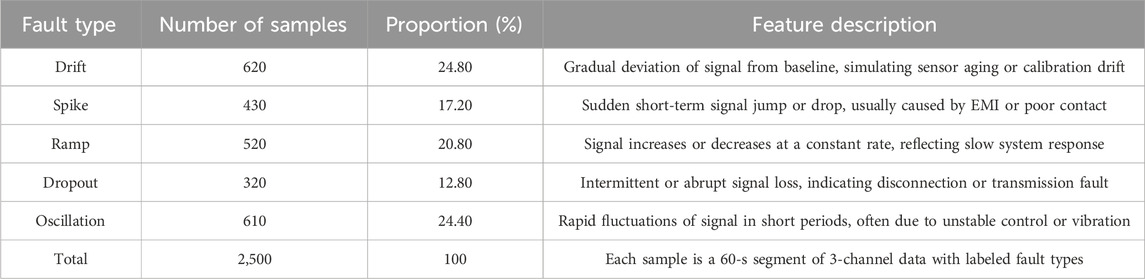
Table 1. Classification statistics and feature description of HVAC sensor fault dataset.

According to Table 1, the performance verification is conducted. Table 2 presents the software and hardware environment information.

Table 2

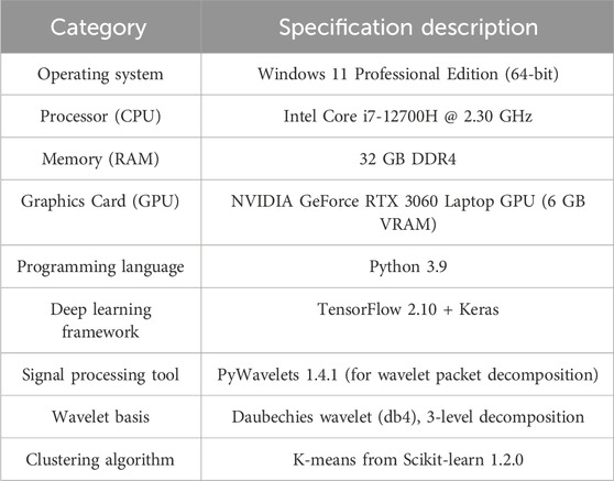
Table 2. Experimental environment and software configuration.

All training and inference processes are completed in a single machine configuration. In the feature modeling stage, the MSR-1DCNN, adopts multi-scale convolutional kernels (sizes 3, 5, and 7) to extract time-domain features. The training rounds are 200, the initial learning rate is 0.001, and the Adam optimizer automatically adjusts the learning step size. In the frequency domain analysis stage, the WPT, uses the db4 basis function from the Daubechies wavelet family for three-layer decomposition to obtain eight sub-band energy features as inputs for K-means clustering analysis.

3.2 Ablation experiment and feasibility verification

To further validate the effectiveness of the proposed MSR-1DCNN model architecture and the contributions of its key modules, we conducted ablation experiments to verify the independent contribution of each structural module to model performance. Using a baseline model without any additional modules as a control group, we added the MSCM, residual connections (Res), and CWCE modules individually or in combination to the model, evaluating their impact on diagnostic performance, as shown in Table 3.

Table 3

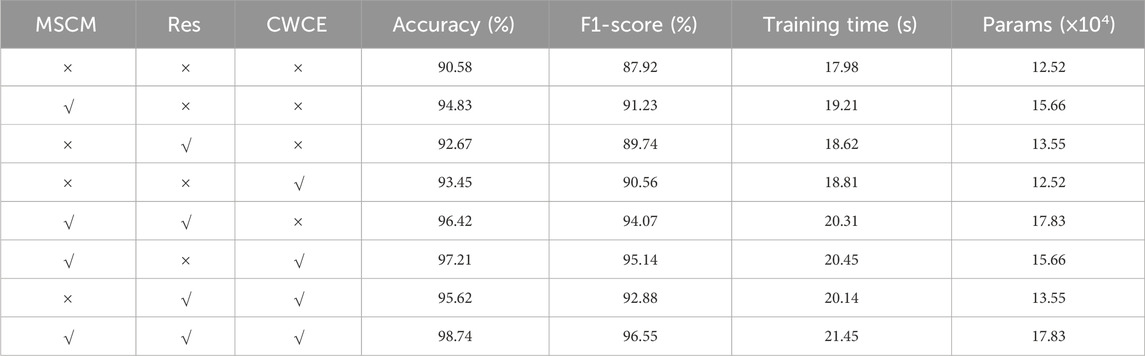
Table 3. Incremental addition ablation experiments of each module.

As shown in Table 3, the baseline model without any additional modules achieved only 90.58% accuracy and 87.92% F1-score, respectively. It had a parameter count of 12.52 × 10⁴ and the shortest training time. With the incremental introduction of each module, model performance improved significantly. The most significant gain was achieved with the MSCM module alone, increasing accuracy by 4.25% and F1-score by 3.31%, demonstrating the positive effects of multi-scale convolution on extracting fault features at different time scales. The Res module alone improved accuracy and F1-score by 2.09% and 1.82%, respectively, primarily due to its role in optimizing gradient transfer and stabilizing network training. While CWCE does not change the number of parameters, it improves classification stability in class imbalance scenarios, increasing accuracy and F1-score by 2.87% and 2.64%, respectively. Combining multiple modules further enhances model performance. The MSCM + CWCE combination approaches the full model in accuracy and F1 score, with only 15.66 × 10⁴ parameters, demonstrating high cost-effectiveness. The MSCM + Res combination performs slightly worse than the MSCM + CWCE combination, but still outperforms the single module. The Res + CWCE combination also shows steady improvement over the baseline. When all three modules are enabled, the model achieves the highest accuracy of 98.74% and an F1 score of 96.55% with 17.83 × 10⁴ parameters. This demonstrates that MSCM provides the strongest feature extraction capabilities and is the core source of performance improvement. CWCE, through class weighting, improves the model’s adaptability to imbalanced samples without increasing the number of parameters. The Res structure enhances gradient propagation and training stability. The rational combination of these three modules achieves an optimal balance between diagnostic accuracy and computational cost.

The performance of different signal modeling methods in fault diagnosis tasks is compared from the perspective of feature extraction. Feature spaces based on the frequency domain features of Raw signal, Fast Fourier Transform (FFT), and WPT are constructed. Three typical clustering algorithms, namely, K-means, Density-Based Spatial Clustering of Applications with Noise (DBSCAN) and Spectral Clustering, are analyzed, as presented in Figure 5.

Figure 5

Figure 5. Feasibility verification of time domain and frequency domain modeling methods. (a) Purity and silhouette coefficient of K-means clustering under different frequency domain features. (b) Diagnostic accuracy and NMI of different clustering methods

According to the clustering results based on K-means algorithm in Figure 5a, WPT performed the best in frequency domain features, with Purity and Silhouette coefficients of 0.9017 and 0.7012, respectively. The clustering accuracy and stability were better than those of FFT and the raw signal. Figure 5b further compares the diagnostic accuracy and Normalized Mutual Information (NMI) of different feature + cluster combinations. The WPT + K-means had the highest accuracy of 92.37% and NMI of 0.853, followed by FFT + K-means and WPT + DBSCAN, while the raw signal + K-means had the worst effect, only 81.24% and 0.622. This indicates that WPT frequency domain features can improve clustering performance and fault recognition performance, and K-means algorithm has more advantages in structured data. Finally, the study further analyzes the fusion effect of MSR-1DCNN model and WPT clustering, as shown in Figure 6.

Figure 6

Figure 6. Fusion analysis of Softmax output and clustering results. (a) Changes in accuracy and Kappa coefficient under different fusion weights α. (b) Comparison of F1-scores between single prediction and fusion prediction for each fault category

From Figure 6a, as $\alpha$ gradually increased from 0.0, the overall performance improved. The best performance was achieved at $\alpha$ = 0.6, with an accuracy of 96.73% and a Kappa coefficient of 0.92. Moderately integrating time-domain Softmax output with frequency-domain clustering results can help suppress noise interference and enhance diagnostic robustness. When $\alpha$ exceeded 0.6, both indicators slightly decreased, indicating that excessive reliance on information from a single source may introduce redundancy or misjudgment. Figure 6b further compares the F1-score performance of single prediction and fusion prediction for different fault types when $\alpha$ = 0.6. The fusion method has the most significant effect on sudden and periodic faults such as Oscillation, Dropout, and Spike, with F1-scores increased by 6.67%, 9.64%, and 6.90%, respectively. Ramp, Drift, and other slowly changing faults, also showed an improvement of 4.40%–5.62%, demonstrating the universality of the fusion strategy.

3.3 Method comparison and performance analysis

To demonstrate the effectiveness of the HVAC fault diagnosis method, performance comparisons are conducted by introducing unimproved 1-D CNN, Bidirectional Long Short-Term Memory (BiLSTM), and Gated Recurrent Unit (GRU) network. Firstly, the diagnostic accuracy and F1-score of four methods are analyzed under different training set ratios, as shown in Figure 7.

Figure 7

Figure 7. Performance comparison of different methods. (a) Comparison of the accuracy of different models in the training set. (b) Comparison of theF1-score of different models in the training set

Figure 7 displays the accuracy and Kappa coefficient of MSR-1DCNN, 1-D CNN, BiLSTM, and GRU at different training ratios. As shown in Figure 7a, MSR-1DCNN consistently maintained optimal accuracy across the entire range, with improvements of 8.71%, 11.97%, and 14.09% compared to 1-D CNN, BiLSTM, and GRU, respectively, at 20% of samples. Under 100% sample conditions, MSR-1DCNN still led by 4.56%–7.67%, indicating its good generalization ability under both small sample and full data conditions. Figure 7b further demonstrates the Kappa coefficient consistency advantage of MSR-1DCNN. The study also evaluated the Receiver Operating Characteristic (ROC) curves of the four methods under Gaussian white noise perturbations with standard deviations of 0%, 10%, 20%, and 30% of the signal amplitude. Noise was superimposed on the original signal to simulate electromagnetic interference, sensor drift, and sampling errors commonly found in HVAC systems. Different amplitudes corresponded to interference scenarios of varying intensities. This is shown in Figure 8.

Figure 8

Figure 8. Robustness verification of different methods. (a) ROC curves of different models under 0% noise. (b) ROC curves of different models under 0% noise. (c) ROC curves of different models under 20% noise. (d) ROC curves of different models under 30% noise.

Figures 8a-d show the changes in fault diagnosis performance under different Gaussian white noise interference (0%, 10%, 20%, and 30%). MSR-1DCNN exhibited the highest true positive rate and area under the curve under all noise conditions. Even when the noise intensity reached 30%, MSR-1DCNN still maintained a high level. In contrast, the performance of 1-D CNN, BiLSTM, and GRU significantly decreased after noise enhancement, and the GRU model performed the worst in the low true positive rate range, indicating its sensitivity to interference signals. Figure 9 presents the inference time and Instantaneous Robustness Drop (IRD) at various noise levels.

Figure 9

Figure 9. Comparative analysis of model inference efficiency and robustness degradation under different noise levels. (a) Comparison of inference time under different noise levels. (b) Comparison of IRD under different noise levels.

In Figure 9a, as the proportion of Gaussian white noise increased, the inference time of MSR-1DCNN increased from 3.12 ms to 3.48 ms, with an increase of 11.5%. In contrast, BiLSTM increased from 5.78 ms to 9.86 ms, with a growth rate of 70.6%, significantly higher than that of MSR-1DCNN. The amplification rates of GRU and 1-D CNN were 17.7% and 13.9%, respectively, both higher than that of MSR-1DCNN, indicating that BiLSTM, GRU, and unimproved 1-D CNN structures are more susceptible to noise interference and affect operational efficiency. In Figure 9b, the IRD value of MSR-1DCNN only increased by 0.010 under 10%–30% noise, while 1-D CNN, BiLSTM, and GRU increased by 0.060, 0.070, and 0.060, respectively. MSR-1DCNN has a stronger anti degradation ability than that of BiLSTM. This indicates that the MSR-1DCNN model has the lowest inference latency among all methods, demonstrating its low computational cost and feasibility for real-time deployment in actual HVAC systems. Furthermore, it demonstrates that the MSR-1DCNN model exhibits superior robustness to interference while maintaining a low computational burden. To further verify the effectiveness and stability of the proposed method, 10 repeated experiments were conducted on four models: MSR-1DCNN, 1-D CNN, BiLSTM, and GRU under the same test set conditions. The experimental results were statistically analyzed using the mean and 95% confidence interval (CI). Details are shown in Table 4.

Table 4

Table 4. Comparison of test set performance of different methods.

Table 4 shows that the MSR-1DCNN achieved a test set accuracy of 97.84%, a significant improvement over the other three methods. MSR-1DCNN also maintained the highest F1 score, precision, and recall, demonstrating that the model has low false positive and false negative rates. Furthermore, the MSR-1DCNN achieved the smallest 95% CI, indicating more stable and reliable results. Beyond the numerical improvements in accuracy, robustness, and computational efficiency, the proposed method has strong practical significance. Its low inference latency and noise resistance make it suitable for real-time HVAC monitoring and fault diagnosis, supporting energy management and equipment maintenance in intelligent buildings. In terms of computational complexity, the MSR-1DCNN has only 17.83×10⁴ parameters and 0.34 G Floating Point Operations (FLOPs), significantly lower than BiLSTM and GRU, and comparable to 1-D CNN, but with higher performance. This demonstrates that the model maintains high accuracy while maintaining low computational cost, making it suitable for deployment in resource-constrained scenarios.

3.4 Extended validation

To further verify the applicability of the proposed MSR-1DCNN method in real-world noise scenarios, four typical noise fault categories were constructed based on noisy HVAC sensor data collected on-site: drift, spike, dropout, and oscillation. Furthermore, the study introduced HVAC machine learning (ML) from Reference (Al-Aomar et al., 2024) and HVAC FDD-Tree from Reference (Patil and Malwatkar, 2024) to compare their performance with the MSR-1DCNN. The results are shown in Table 5.

Table 5

Table 5. Comparison of classification accuracy under real noisy fault data.

Table 5 shows that for drift faults, the MSR-1DCNN achieves an accuracy of 95.83%, an improvement of 9.69% and 7.54% over HVAC-ML and HVAC-FDD-Tree, respectively. The MSR-1DCNN also demonstrates superior performance in noise fault categories such as spike, dropout, and oscillation. This demonstrates that the MSR-1DCNN possesses superior fault identification capabilities and stability in real-world noise environments, particularly in spike and dropout noise scenarios characterized by strong randomness and localized perturbations. This is likely due to the multi-scale feature extraction and WPT band enhancement mechanism employed by the MSR-1DCNN, which effectively suppresses noise interference and improves signal discrimination, thereby enhancing model robustness and accuracy.

4 Conclusion

An MSR-1DCNN-wavelet clustering joint model was constructed to address the poor generalization of small samples, weak noise resistance, and high inference delay in HVAC sensor fault diagnosis. Experiments showed that in extreme scenarios where the training set only accounted for 20%, the accuracy of MSR-1DCNN still reached 85.47%, with an average improvement of 9.18% compared to the baseline. Under 30% Gaussian noise, the IRD index was superior to BiLSTM, and the inference time increase was only 1/6 of BiLSTM, demonstrating excellent robustness and real-time performance. The HVAC diagnosis method can maintain a low computational burden and has superior anti-interference robustness. However, the research is still limited to offline batch processing scenarios and has not yet been verified in an online incremental learning environment. Furthermore, cross-building migration testing has not been introduced, and the generalization boundaries of the model still need to be further clarified. Future work will be directed towards edge GPU deployment, enabling lightweight inference and exploring online continuous learning and cross-scenario adaptability. In terms of online incremental learning, a sliding window and small-batch dynamic update mechanism will be adopted to enable the model to adapt to new data and failure modes without repeated training. In terms of domain adaptation, feature alignment and transfer learning will be used to reduce the differences in data distribution across different buildings, and a cross-building migration benchmark will be constructed to explore domain adaptive fine-tuning strategies to improve the generalization and practicality of HVAC sensor fault detection.

Data availability statement

The original contributions presented in the study are included in the article/supplementary material, further inquiries can be directed to the corresponding author.

Author contributions

LW: Conceptualization, Data curation, Formal Analysis, Writing – original draft, Writing – review and editing. RH: Investigation, Methodology, Writing – original draft, Writing – review and editing. JL: Software, Supervision, Writing – original draft, Writing – review and editing.

Funding

The author(s) declare that no financial support was received for the research and/or publication of this article.

Conflict of interest

The authors declare that the research was conducted in the absence of any commercial or financial relationships that could be construed as a potential conflict of interest.

Generative AI statement

The author(s) declare that no Generative AI was used in the creation of this manuscript.

Any alternative text (alt text) provided alongside figures in this article has been generated by Frontiers with the support of artificial intelligence and reasonable efforts have been made to ensure accuracy, including review by the authors wherever possible. If you identify any issues, please contact us.

Publisher’s note

All claims expressed in this article are solely those of the authors and do not necessarily represent those of their affiliated organizations, or those of the publisher, the editors and the reviewers. Any product that may be evaluated in this article, or claim that may be made by its manufacturer, is not guaranteed or endorsed by the publisher.

References

Abrazeh, S., Mohseni, S. R., Zeitouni, M. J., Parvaresh, A., Fathollahi, A., Gheisarnejad, M., et al. (2022). Virtual hardware-in-the-loop FMU co-simulation based digital twins for heating, ventilation, and air-conditioning (HVAC) systems. IEEE Trans. Emerg. Top. Comput. Intell. 7 (1), 65–75. doi:10.1109/TETCI.2022.3168507

CrossRef Full Text | Google Scholar

Ahmadzadeh, M., Zahrai, S. M., and Bitaraf, M. (2025). An integrated deep neural network model combining 1D CNN and LSTM for structural health monitoring utilizing multisensor time-series data. Struct. Health Monit. 24 (1), 447–465. doi:10.1177/14759217241239041

CrossRef Full Text | Google Scholar

Al-Aomar, R., AlTal, M., and Abel, J. (2024). A data-driven predictive maintenance model for hospital HVAC system with machine learning. Build. Res. and Inf. 52 (1-2), 207–224. doi:10.1080/09613218.2023.2206989

CrossRef Full Text | Google Scholar

Arkin, E., Yadikar, N., Xu, X., Aysa, A., and Ubul, K. (2023). A survey: object detection methods from CNN to transformer. Multimedia Tools Appl. 82 (14), 21353–21383. doi:10.1007/s11042-022-13801-3

CrossRef Full Text | Google Scholar

Gao, W., Yu, L., Tan, Y., and Yang, P. (2022). MSIMCNN: multi-scale inception module convolutional neural network for multi-focus image fusion. Appl. Intell. 52 (12), 14085–14100. doi:10.1007/s10489-022-03160-9

CrossRef Full Text | Google Scholar

Groumpos, P. P. (2023). A critical historic overview of artificial intelligence: issues, challenges, opportunities, and threats. Artif. Intell. Appl. 1 (4), 181–197. doi:10.47852/bonviewAIA3202689

CrossRef Full Text | Google Scholar

Huang, M., and Liao, Y. (2022). Development of an indoor environment evaluation model for heating, ventilation and air-conditioning control system of office buildings in subtropical region considering indoor health and thermal comfort. Indoor Built Environ. 31 (3), 807–819. doi:10.1177/1420326X211035550

CrossRef Full Text | Google Scholar

Huang, H., Li, L., Liu, S., Hao, B., and Ye, D. (2024). Wavelet packet transform and deep learning-based fusion of audio-visual signals: a novel approach for enhancing laser cleaning effect evaluation. Int. J. Precis. Eng. Manufacturing-Green Technol. 11 (4), 1263–1278. doi:10.1007/s40684-023-00589-2

CrossRef Full Text | Google Scholar

Iqbal, M., and Madan, A. K. (2022). CNC machine-bearing fault detection based on convolutional neural network using vibration and Acoustic signal. J. Vib. Eng. and Technol. 10 (5), 1613–1621. doi:10.1007/s42417-022-00468-1

CrossRef Full Text | Google Scholar

Moumene, I., and Ouelaa, N. (2022). Gears and bearings combined faults detection using optimized wavelet packet transform and pattern recognition neural networks. Int. J. Adv. Manuf. Technol. 120 (7), 4335–4354. doi:10.1007/s00170-022-08792-2

CrossRef Full Text | Google Scholar

Niu, J., Li, H., Zhang, C., and Li, D. (2021). Multi-scale attention-based convolutional neural network for classification of breast masses in mammograms. Med. Phys. 48 (7), 3878–3892. doi:10.1002/mp.14942

PubMed Abstract | CrossRef Full Text | Google Scholar

Patil, M. S., and Malwatkar, G. M. (2024). A compressive study on fault detection and diagnosis for reliable operation of HVAC, energy buildings and machineries. Reliab. Theory and Appl. 19 (1), 631–649. doi:10.24412/1932-2321-2024-177-631-649

CrossRef Full Text | Google Scholar

Qiu, S., Cheng, X., Lu, H., Zhang, H., Wan, R., Xue, X., et al. (2023). Subclassified loss: rethinking data imbalance from subclass perspective for semantic segmentation. IEEE Trans. Intelligent Veh. 9 (1), 1547–1558. doi:10.1109/TIV.2023.3325343

CrossRef Full Text | Google Scholar

Song, X., Cong, Y., Song, Y., Chen, Y., and Liang, P. (2022). A bearing fault diagnosis model based on CNN with wide convolution kernels. J. Ambient Intell. Humaniz. Comput. 13 (8), 4041–4056. doi:10.1007/s12652-021-03177-x

CrossRef Full Text | Google Scholar

Sousan, S., Fan, M., Outlaw, K., Williams, S., and Roper, R. L. (2022). SARS-CoV-2 detection in air samples from inside heating, ventilation, and air conditioning (HVAC) systems—Covid surveillance in student dorms. Am. J. Infect. Control 50 (3), 330–335. doi:10.1016/j.ajic.2021.10.009

PubMed Abstract | CrossRef Full Text | Google Scholar

Wang, Z. C., Li, D., Cao, Z. W., Gao, F., and Li, M. J. (2024). A modified transformer and adapter-based transfer learning for fault detection and diagnosis in HVAC systems. Energy Storage Sav. 3 (2), 96–105. doi:10.1016/j.enss.2024.02.004

CrossRef Full Text | Google Scholar

Yan, K., and Zhou, X. (2022). Chiller faults detection and diagnosis with sensor network and adaptive 1D CNN. Digital Commun. Netw. 8 (4), 531–539. doi:10.1016/j.dcan.2022.03.023

CrossRef Full Text | Google Scholar

Zhang, Q., and Deng, L. (2023). An intelligent fault diagnosis method of rolling bearings based on short-time fourier transform and convolutional neural network. J. Fail. Analysis Prev. 23 (2), 795–811. doi:10.1007/s11668-023-01616-9

CrossRef Full Text | Google Scholar

Zhao, Z., and Jiao, Y. (2022). A fault diagnosis method for rotating machinery based on CNN with mixed information. IEEE Trans. Industrial Inf. 19 (8), 9091–9101. doi:10.1109/TII.2022.3224979

CrossRef Full Text | Google Scholar