Investigating the impact of imperfections around a wellbore on liner deformation during hydraulic fracturing

It is essential to maintain the integrity of liner–cement–formation in the well completion and production stages. However, large liner deformations have been extensively experienced during hydraulic fracturing operations in carbonate formations. This work reveals that local collapse and burst may cause the liner to deform during hydraulic fracturing operations. The stressing and deformation of liners are investigated using numerical simulation at two levels. First, a stand-alone liner is compressed from the outside or expanded from the inside to calibrate the plastic parameters by matching the collapse and burst pressures in the liner’s technical specifications. The influence of the non-uniformity of loads and confinement on the liner’s bearing capacity is then investigated. Second, the influence of imperfections in the cement or cavities in the formation on liner deformation in a liner–cement–formation system is explored. Simulation results indicate that the hydraulic communication between the cavities, vugs, or other imperfections in formation or cementing around a liner and hydraulic fractures can introduce an uneven load on the liner, subsequently threatening the integrity of the liner–cement–formation system and causing a large deformation in the liner. This mechanism has not received much attention in the practical hydraulic fracturing operation design.

1 Introduction

Hydraulic fracturing is an important technology in the extraction of resources and energy from subsurface in oil and gas, mining, and geothermal industries (Wang et al., 2014; Montgomery and Smith, 2010; Moska et al., 2021). In the oil and gas industry, multistage hydraulic fracturing and horizontal drilling are the critical technologies that have made it economically feasible to produce hydrocarbons from unconventional source rocks (Waters et al., 2009). Liner deformation is frequently experienced during hydraulic fracturing in unconventional source rocks, which in many cases can result in serious downhole issues, such as restricted access for interventions, loss of well integrity, or even premature well abandonment. Maintenance of wellbore integrity is essential at every stage of well life, including drilling, completion, and production (Han et al., 2015; Li et al., 2024). To prevent or mitigate the large liner deformation issues, it is necessary to understand the dominant mechanisms behind the liner deformation in various engineering scenarios.

In general, a liner can deform and fail in buckling, axial compression collapse, and radial compression collapse. Both buckling and axial compression collapse are caused by axial load and poor radial constraint (Vudovich et al., 1988). Naturally existing fractures, vugs, and cavities in carbonate formations will relax the radial support on the liner. Low-efficiency cement placement in the annulus can result in a weakened cement sheath, reducing support from the formation (Furui et al., 2010; Yousuf et al., 2021). For example, a casing string without continuous cementing throughout its length can easily run into axial buckling during reservoir compaction. The lateral support may also be relaxed by enlarged cavities created by cluster perforation, high-volume acid treatment, sand production, and reservoir compaction (Vudovich et al., 1988; Kiran et al., 2017). The radial compression collapse is caused by high stress transferred from the formation after the cement hardens or the formation depletes (Wilson et al., 1979; Peng et al., 2007; Zhang et al., 2019; Li et al., 2023).

Debonding and crack development along the liner–cement and cement–formation interfaces can be caused by shrinkage of the cement sheath due to its curing process or deterioration of the cement under downhole conditions (Wang and Taleghani, 2014; De Andrade and Sangesland, 2016; Guo et al., 2018). They may also be induced by differential stress between the liner and cement during stimulation or temperature cycles (e.g., in an enhanced geothermal system), and many other factors, such as poor cementing, thermal stress, wellbore inclination, liner eccentricity, or mud cake formed on the wellbore wall during drilling (Dusseault et al., 2001). Due to delamination, an annular fracture may develop along the cement–formation interface during hydraulic fracturing (Wang and Taleghani, 2014; Kiran et al., 2017). The cracks along the liner–cement and cement–formation interfaces provide pathways for fluid migration, leading to a great risk of liner deformation and collapse (De Andrade and Sangesland, 2016).

Cement plays an important role in maintaining wellbore integrity. Cement can fail in both the completion (e.g., hydraulic fracturing) and production stages (Mou et al., 2023). The failure mode can be radial cracking or compressive shear yielding. The failure can be induced by environmental change, strength reduction over time, or chemical degradation (Wang and Taleghani, 2014; Guo et al., 2018).

In this study, we investigate the possibility of imperfections around the wellbore in a deforming and failing liner during hydraulic fracturing (e.g., in carbonate formations). The cavities can be introduced by a poor-quality cementing job or simply be pre-existing vugs in the carbonate formation (Zhang et al., 2019). It is further assumed that the cavities can hydraulically communicate with fractures through natural fractures during a hydraulic fracturing operation. To our best knowledge, this mechanism has rarely been studied in the literature. The investigations are conducted using numerical simulation, which can consider the drilling, construction, and production phases step by step. The problem of liner–cement–formation interaction is modeled in plane strain mode, and the liner–cement and cement–formation interfaces are modeled as elastoplastic contacts.

This article is organized as follows: in Section 2, we build a set of stand-alone liner models for calibrating the mechanical properties of a liner material with a liner’s technical specifications and test the behaviors of the liner under several idealized loading modes. In Section 3, we construct a liner–cement–formation interaction model and experiment with the responses of the system in several hypothesized scenarios of cavities. Summary comments are provided in Section 4.

2 Stand-alone liner models

In this work, the commercial computational software FLAC version 7.0 is adopted to perform the numerical simulations. FLAC is a two-dimensional explicit finite volume method-based computational geomechanics software program distributed by Itasca (2011). This program simulates the mechanical behaviors of structures built of soil, rock, and other materials that may experience plastic flow when their yielding limits are reached. In FLAC, each calculation step solves the equation of motion at all grid points and constitutive laws at all elements. The equations are solved explicitly, and numerical stability is ensured by rigorously setting the timestep following the principle that the wave propagating distance over one timestep will be less than the size of the smallest element in the model. One unique feature of FLAC is the dynamic relaxation method, which solves full dynamic equations even for static problems; the kinetic energy is dissipated by damping. One salient advantage of this approach is that it can model engineering problems that include large deformation (Liu and Han, 2005).

Four stand-alone liner models are presented in this section. The first and second models (see Figure 1) have a uniform compressive pressure applied on the inside and outside surfaces of the stand-alone liner, respectively. In the third model, the liner is loaded by a compressive pressure unidirectionally, while in the fourth model, the liner has a non-uniform compressive pressure on the external boundary, as illustrated in Figure 2.

Figure 1

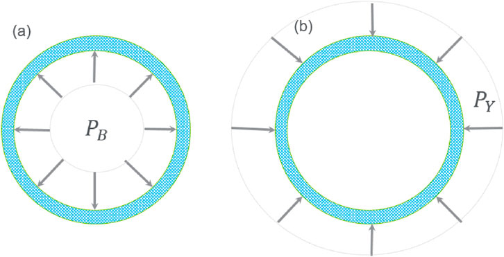
Figure 1. Stand-alone ring structure liner model with (a) uniform internal compressive load, ${\mathit{P}}_{\mathit{B}}$, acting outward inside the pipe, and (b) uniform external compressive load, ${\mathit{P}}_{\mathit{Y}}$, acting inward on the outside of the pipe.

Figure 2

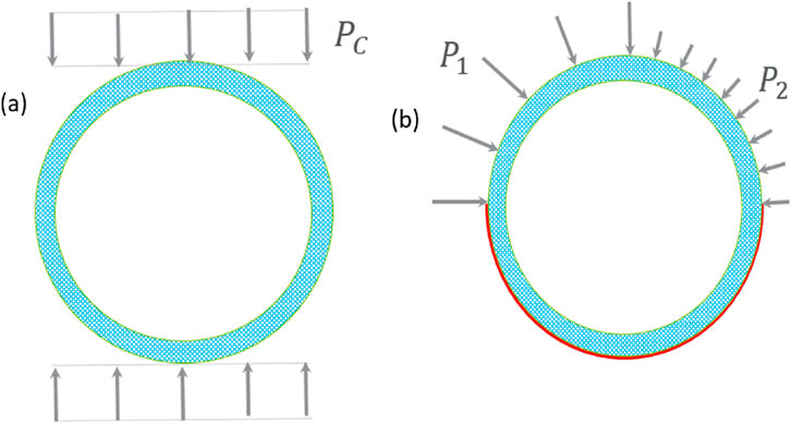
Figure 2. Stand-alone ring structure liner model with (a) unidirectional compressive load, ${\mathit{P}}_{\mathit{C}}$, acting downward on the top of the pipe, and (b) non-uniform external compressive loads, ${\mathit{P}}_1$ and ${\mathit{P}}_2$, acting radially and inward on the outside of the pipe.

The loading conditions in the first two models correspond to the testing configurations in the technical specifications of the liner pipe, so they can be used to calibrate the mechanical properties of the liner material. The calibrated material properties and model are then used to predict the bearing capacity of the liner under different loading conditions, such as those in the third and fourth models.

2.1 Model calibration

The outer diameter (OD), inner diameter (ID), Young’s modulus, Poisson’s ratio, burst, and compressive yield pressures of a typical steel liner are provided in Table 1. It should be noted that the buckling external pressure of the liner (pipe) can be estimated using the following equation:

$P_{cr}=\frac{E}{4\left(1-v^2\right)}{\left(\frac{t}{r}\right)}^3,(1)$

where $r$ is the pipe radius, $t$ is the pipe thickness, $E$ is the Young’s modulus, and v is the Poisson’s ratio of the material. Substituting values for these variables into Equation 1 gives 240 MPa, which is close to the yield pressure given in the pipe specifications.

Table 1

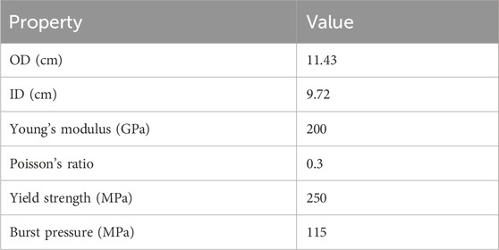
Table 1. Geometric and mechanical properties of the liner.

We built a ring solid element model to determine the tensile and compressive strengths of the liner material through performing numerical simulations of burst and yield tests, that is, Model 1a and Model 1b in Figure 1. The computational mesh of the stand-alone liner model is displayed in Figure 3. The uniform mesh has 10 elements in the radial direction and 120 elements in the tangential direction. Note, the resolution of this mesh is fine enough to accurately capture the mechanical response of the pipe, as verified by comparing the numerical results with the analytical stress solution of a hollow cylinder in its elastic response range. Note also that more “advanced” models, like the von Mises model with strain hardening, can more accurately capture the detailed mechanical response of the steel material. However, in this work, we are only interested in capturing the loading capacity (but not the detailed stress–strain responses) of steel pipe in compressive and tensile failure modes. A simple model, such as Mohr–Coulomb and Drucker–Prager, that can capture the compressive and tensile loading limits of steel pipe through calibration, shall be sufficient to serve the intended modeling purpose. Here, the liner is modeled as a frictionless Mohr–Coulomb type material with limited cohesion and tensile strength. The elastic properties listed in Table 1 are assigned to the model directly. The cohesive and tensile strengths of the steel material are to be determined by calibration. Note, these two models also test whether the resolution of the selected mesh in the stand-alone model is fine enough to capture the mechanical responses of the liner structure.

Figure 3

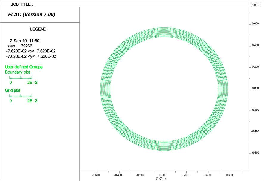
Figure 3. Computational mesh of the stand-alone ring structure liner model.

2.1.1 Burst test

In this simulation, a 100 MPa pressure is applied on the inside surface of the liner, and then the model is run to equilibrium. Figure 4a shows that the compressive radial stress decreases radially, and the maximum value occurs at the inner boundary, which is equivalent to an internal loading pressure of 100 MPa. Figure 4b indicates that the tangential stress is in tension everywhere in the liner, and the element on the inner boundary has a maximum value of approximately 620 MPa. Note that in FLAC, stress is positive in tension and negative in compression.

Figure 4

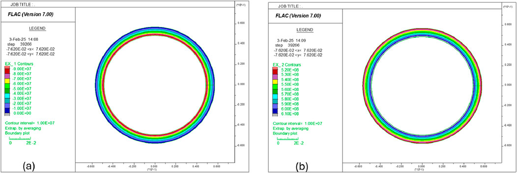
Figure 4. Distribution of (a) radial stress and (b) tangential stress in the liner under internal pressure of 100 MPa.

Next, the pressure inside the liner is increased gradually while the simulation is progressing. Figure 5 displays the plastic yielding occurring at the internal pressure of 113 MPa in Figure 5a and the monitored unbalanced force in the system versus the applied inside pressure in Figure 5b. The response of the system is quiet; that is, the unbalanced force is very low at the beginning. The first spike of the unbalanced force appears when the internal pressure reaches approximately 113 MPa, which corresponds to a sudden release of kinetic energy induced by newly generated tensile cracks initiating in the elements (Han et al., 2022). This pressure is very close to the burst pressure of 115 MPa provided in Table 1. Note, for this simulation, the tensile strength of the liner is set to 700 MPa, which gives a very accurate prediction of its burst pressure.

Figure 5

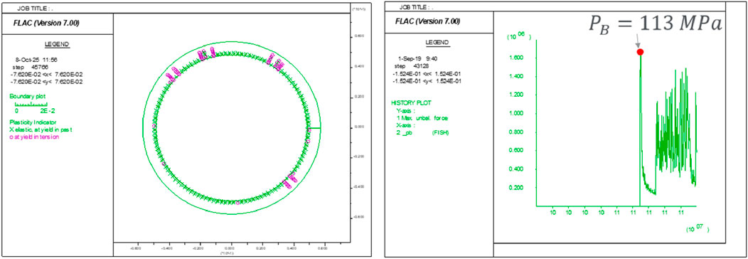
Figure 5. (a) Plastic yielding status at the internal pressure of 113 MPa and (b) the history of unbalanced force in the system versus applied internal pressure.

2.1.2 Radial collapse test

The magnitude of the compressive strength of a steel material could be close to its tensile strength. In the external pressure test model, the computational mesh and mechanical properties of the liner are the same as those of the internal pressure test model described above. The cohesive strength of the liner is set to 700 MPa. The simulation is also performed over two stages. In the first stage, a 100 MPa pressure is applied at the outer boundary of the liner, and the model is run to equilibrium. The resulting radial stress and tangential stress distributions in the liner are presented in Figure 6. The radial stress is in compression everywhere, and its magnitude increases radially and reaches a maximum value of 100 MPa at the outer boundary. The tangential stress is also in compression everywhere, but its magnitude decreases radially, and its maximum value (approximately 720 MPa) occurs at the inner boundary.

Figure 6

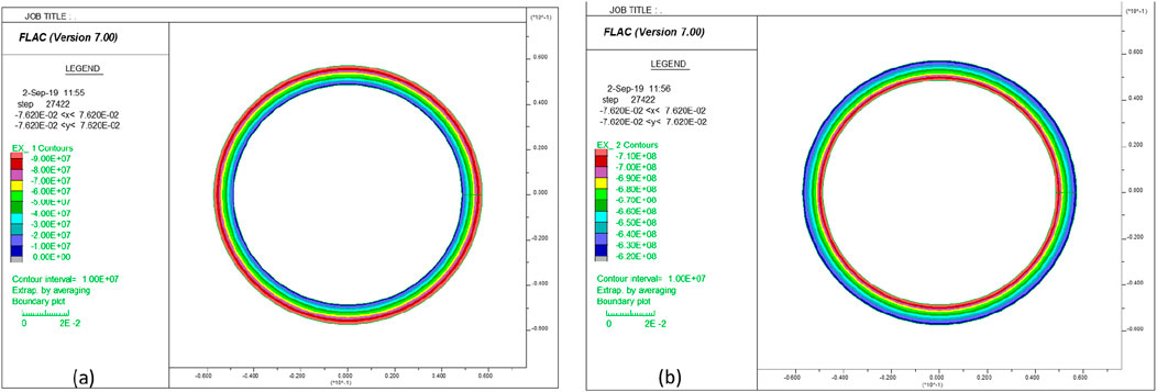
Figure 6. Distribution of (a) radial stress and (b) tangential stress in the liner under an external pressure of 100 MPa.

In the second stage, the applied pressure on the external boundary is increased gradually as the simulation progresses. The plastic yielding status at the external pressure of 220 MPa is displayed in Figure 7a. As seen, the compressive shear yielding initiates from the inner side, where the stress and progressively expands outward. The monitored histories of unbalanced force in the system and applied external pressure are presented in Figure 7b, which shows that, unlike the abrupt kinetic energy emitted by tensile cracking (see Figure 5), in the external compression test, the kinetic energy increases consistently and stably after the compressive shear yielding starts. The point where the kinetic energy starts to deviate from the horizontal line (i.e., the red dot in Figure 7) corresponds to the yield pressure of the liner. The yield pressure of 230 MPa predicted by the model is close enough to the provided yield pressure of 250 MPa listed in Table 1.

Figure 7

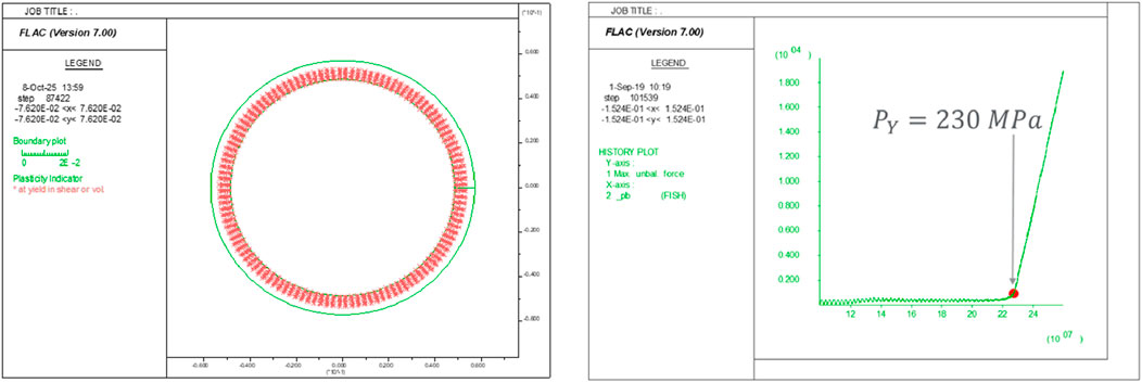
Figure 7. (a) Plastic yielding status at the external pressure of 220 MPa and (b) the history of the unbalanced force in the system versus applied external pressure.

2.2 Model prediction

The burst pressure and yield pressure of the liner are quite high. The integrity of this liner should not be a problem for most commonly encountered engineering conditions, such as borehole and completion depth, in situ stresses, etc. However, it must be kept in mind that both burst pressure and collapse yield pressure are measured under uniformly distributed radial loads, which is an extreme idealization. In the real downhole environment, because of heterogeneity, fractures and cavities in the formation, unequal in situ stresses, imperfect cementing jobs, and leakage of fluid in hydraulic fracturing stimulation, etc., the load on a liner is non-uniform in general. In the subsections below, we will experiment with how the non-uniformity of the load affects the bearing capacity of the liner in two situations.

2.2.1 Unidirectional compression test

The unidirectional compression test is conducted on the model that has been calibrated with burst and yield pressures as described above. The simulation procedure is similar to the yield test. The major difference is that the compressive external pressure is only applied in the y-direction, as illustrated in Figure 2a. Because it is not clear what the yield pressure will be in this loading configuration, the applied pressure starts from zero and increases gradually as the simulation progresses.

Figure 8a shows the history of the unbalanced force (kinetic energy) versus the applied compressive pressure monitored in the simulation. The first spike of kinetic energy is observed when the pressure reaches 52 MPa, which corresponds to the failure compressive pressure. It is interesting to observe that the liner actually fails in tensile crack mode, although a compressive load is applied in the y direction as an external pressure boundary condition. Figure 8b indicates that at a compressive pressure of 53 MPa, tensile cracks initiate from the crown and invert areas on the inner boundary and lateral areas on the outer boundary.

Figure 8

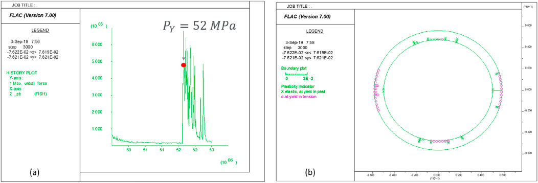
Figure 8. (a) History of unbalanced force in the system versus applied compression pressure and (b) plastic state in the liner under compression pressure of 56 MPa.

Figure 9a shows that the tangential stress is in tension in the crown and invert areas on the inner boundary and lateral areas on the outer boundary, which confirms the failure pattern in Figure 8b. Figure 9b demonstrates that the closure of the liner is approximately 2 mm at the compression pressure of 56 MPa. Clearly, as demonstrated in the unidirectional compression test simulation, the bearing capacity of the liner can be much lower than its yield stress when the liner is subjected to non-uniformly distributed external loads. Overall, this test shows that the failure pressure of the same liner (i.e., 52 MPa) under unidirectional compression loading conditions is less than 25% of its yield pressure (230 MPa) under uniform external compression loading.

Figure 9

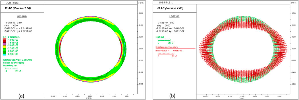
Figure 9. (a) Tangential stress distribution and (b) displacement vectors in the liner under a compression pressure of 56 MPa.

2.2.2 Bimodal compression test

In the scenario sketched in Figure 2b, the bottom half outer boundary of the liner is fixed so it cannot move in either direction; the left and right sides of its top half outer boundary are subjected to pressures with different magnitudes. This situation might be more representative of the loading condition that a liner is experiencing after a poor-quality cementing job is finished.

Taking the liner model created and calibrated above and assuming the magnitude of P₂ is equal to half of P₁ and fixing both x- and y- at the bottom half of the outer boundary, the simulation indicates that tensile cracks start to develop when P₁ reaches 77 MPa, as shown in Figure 10a. Figure 10b shows that the tensile yielding takes place near the crown area (where the applied pressure on the outer boundary transits) and the right lateral area along the inner boundary. Figure 11a confirms the tangential stress is in tension in these two areas. Figure 11b displays the deformation pattern of the liner in this non-uniform loading condition; that is, the upper left part deforms inward, and the upper right part deforms outward.

Figure 10

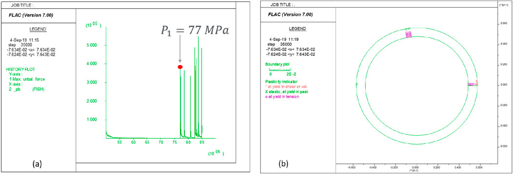
Figure 10. (a) History of unbalanced force in the system versus applied compression pressure P₁; (b) plastic state in the liner under compression of P₁ at 85 MPa.

Figure 11

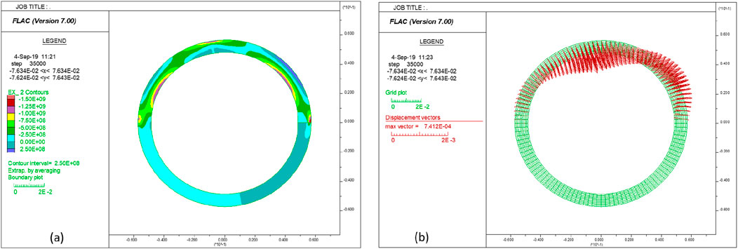
Figure 11. (a) Tangential stress distribution and (b) displacement vectors in the liner under the compression of P₁ at 85 MPa.

If the simulation continues with a gradual increase in the applied pressure on the top half of the liner, the deformation will continue to increase. Figure 12a shows the deformed liner when the left side pressure P₁ reaches 115 MPa (and P₂ is 57.5 MPa). The closure of the top liner is approximately 1.25 cm (0.5 inches). Figure 12b shows that the tensile yielding takes place at five locations at this stage.

Figure 12

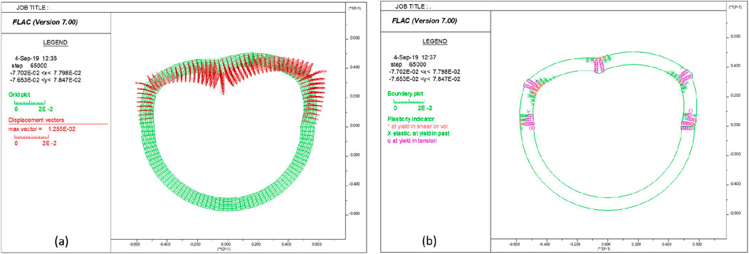
Figure 12. (a) Displacement vectors and (b) plastic state in the liner under the compression of P₁ at 115 MPa.

3 Liner–cement–formation models

In this section, we study the deformation and failure of a liner in a horizontal well. The borehole diameter is 14.92 cm (4.875 inches). The inner layer is the liner. Its geometric and mechanical properties are listed in Table 1. The annulus between the borehole wall and the liner is filled with cementing material. The mechanical properties of the cement and formation rock are listed in Table 2. The borehole is drilled in the minimum horizontal stress direction. The vertical stress (${\sigma }_V$) is $117$ MPa; the maximum horizontal stress (${\sigma }_H$) is $138$ MPa; the minimum horizontal stress (${\sigma }_h$) is $93.5$ MPa; the reservoir pore pressure ($P_p$) is $66.7$ MPa; the fluid pressure inside the borehole and liner is ($P_w$) is $47.8$ MPa; the maximum bottom-hole pressure during hydraulic fracturing ($P_{HF}$) is $138$ MPa.

Table 2

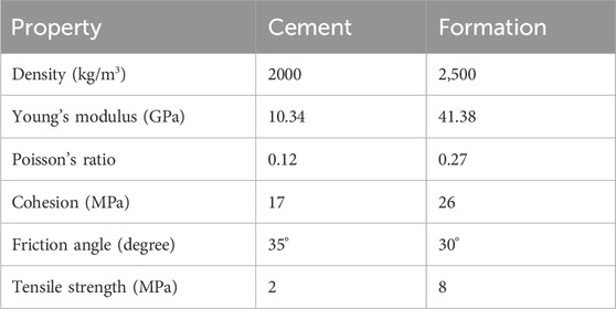
Table 2. Mechanical properties of the cement and formation.

In the downhole condition, the liner is loaded by both internal fluid pressure and mechanical and/or fluid pressure on the outer boundary. The higher the external confining pressure, the higher the burst pressure. In this studied case, an extreme situation is that the cement job is extremely poor and does not take any load, and then the outer boundary of the liner is loaded by fluid pressure in the annulus between the liner and the formation (see Figure 13a). To be conservative, the pressure in the annulus is assumed to be the same as the wellbore pressure, that is, P_o = 47.8 MPa.

Figure 13

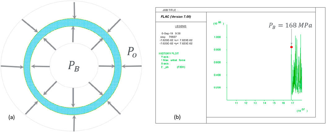
Figure 13. (a) Burst pressure under a confining stress P_o; (b) burst pressure of the liner under an external pressure of 47.8 MPa.

The burst test model in the first section is re-run with applied external confining pressure. The simulation predicted that the burst pressure of the liner under external confining stress of 47.8 MPa is approximately 168 MPa (see Figure 13b). This burst pressure is much higher than the maximum bottom-hole pressure (138 MPa) experienced by the liner during the hydraulic fracturing treatment. Therefore, the liner is not expected to fail in burst mode during hydraulic fracturing.

Model 1(b) indicated that the yield pressure (i.e., 230 MPa) of this liner is nearly 100 MPa higher than the maximum in situ stress and maximum bottom-hole pressure (i.e., 138 MPa). If there is fluid pressure acting inside the liner, the yield pressure is even higher than 230 MPa. For example, simulation indicated that, with a fluid pressure of 47.8 MPa inside the liner, the liner starts to collapse at a uniform external pressure of 275 MPa.

Therefore, for the stress and pressure that is experienced during the hydraulic fracturing in this borehole segment, the liner should not yield or collapse if the loads on its outer boundary are uniformly distributed. On the other hand, as predicted by stand-alone liner models with non-uniform loads, the yield stress of the liner can reduce very sharply if the loads on its outer boundary are non-uniform. For example, for the unidirectional compression test, the yield stress can drop to 52 MPa. In order to evaluate the deformation and integrity of the liner, it is critical to determine the load distributions on its outer boundary.

If the loads acting on the inner and outer boundaries of the liner pipe are known, the deformation and integrity of the liner can be evaluated directly using the liner model calibrated above. The liner is filled with fluid all the time, so the load acting on the inner boundary is a uniform fluid pressure, although its magnitude may change during completion, stimulation, and production. The magnitude and distribution of loads on the outer boundary of the liner, however, are extremely difficult to determine because of too many influential factors. For example, they can be affected by near-wellbore stresses and pore pressure, borehole drilling quality, the cementing procedure and quality, the mechanical response and status of cement, the connection between the cement and the liner, the connection between the cement and the formation, the stimulation operation, production progress (e.g., depletion), and other factors. To estimate loads and their distributions on the outer boundary with relative accuracy, it is necessary to build a liner–cement–formation interaction system and study the evolution of the stresses and deformation under the drive of operations at completion, stimulation, and production stages.

Considering the complexity and uncertainties in various downhole operations, it is challenging, if not impossible, to accurately mimic and capture the influence of so many affecting factors in all the operations. Instead, in the modeling work below, we choose to approximately capture the impact of major engineering processes on the load distribution around the liner in the model buildup and initialization stage, then investigate how voids in cement or formation layers, which are believed to play the primary role in deforming the liner, affect the liner deformation and integrity.

The computational mesh for modeling the liner–cement–formation system is displayed in Figure 14. Overall, the mesh has 80 elements in the radial direction and 120 elements in the circumferential direction. The inner layer is identical to the mesh calibrated in the stand-alone liner models in the previous section. The middle layer spans radially from 11.43 cm to 14.92 cm (i.e., the annulus between the liner and the borehole wall). The outer layer extends radially to 50.8 cm (i.e., 20 inches). In the radial direction, the liner layer has 10 elements, the cement has 10 elements, and the formation layer has 60 elements.

Figure 14

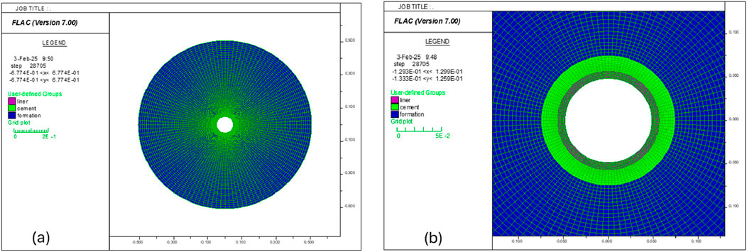
Figure 14. Computational mesh of liner–cement–formation model: (a) full view; (b) close-up view.

3.1 Model verification

3.1.1 Analytical solution

The exact stress solutions of a multi-layered elastic hollow cylinder subjected to uniform pressures on the inner and outer surfaces were analytically solved by Shi et al. (2007). The system is illustrated in Figure 15a, and the flowchart of implementing the analytical solutions in Mathematica is shown in Figure 15b. The hole radius is $r_0$. Arbitrarily, the ith layer is defined by its inner radius $r_{i-1}$, outer radius $r_i$, Young’s modulus $E_i$, and Poisson’s ratio $v$. $Q$ and $q$ are the pressure on the outer and inner surface, respectively.

Figure 15

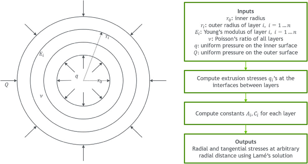
Figure 15. (a) A concentric multi-layer elastic medium subjected to uniform loads on the inside and outside surfaces, and (b) a flowchart to implement the analytical solutions of Shi et al. (2007) in Mathematica.

The liner–cement–formation is a three-layered hollow cylinder. In the elastic response range and under uniform pressure loading conditions, the stresses on the liner–cement and cement–formation interfaces can be evaluated using the analytical solutions of Shi et al. (2007) and Han et al. (2024). Referring to Figure 15, the geometric parameters of the liner–cement–formation system are:

$d_0$ = 9.72 cm (inner diameter of liner);

$d_1$ = 11.43 cm (outer diameter of the liner, also the inner diameter of the cement);

$d_2$ = 14.92 cm (outer diameter of the cement layer, also the inner diameter of the formation); and

$d_3$ = 50.8 cm (outer diameter of the formation layer).

The Young’s moduli and Poisson’s ratios of these layers are (see Tables 1, 2):

Liner layer: $E_1$ = 200 GPa; $v_1$ = 0.3;

Cement layer: $E_2$ = 10.34 GPa; $v_2$ = 0.3; and

Formation layer: $E_3$ = 41.38 GPa; $r_3$ = 0.3.

The uniform pressures on the inner and outer surfaces are:

$\mathit{q}$ = 50 MPa and

$\mathit{Q}$ = 140 MPa.

With the above input parameters, the analytical solutions report that the stress on the interface between the liner and cement (${\mathit{P}}_{\mathit{l}\mathit{c}}$) is 114.6 MPa, and the stress on the interface between the cement and formation (${\mathit{P}}_{\mathit{c}\mathit{f}}$) is 105.3 MPa, that is:

${\mathit{P}}_{\mathit{l}\mathit{c}-\mathit{a}\mathit{n}\mathit{a}}=114.6\text{\hspace{0.17em}MPa},$

${\mathit{P}}_{\mathit{c}\mathit{f}-\mathit{a}\mathit{n}\mathit{a}}=105.3\text{\hspace{0.17em}MPa}.$

3.1.2 Numerical simulation

After the computational mesh (see Figure 14) is generated, and the elastic materials of liner, cement, and formation are assigned to the corresponding regions in the mesh, a pressure of 50 MPa is applied on the inside surface of the liner, and a pressure of 140 MPa is applied on the outside surface of the formation layer. The model is then solved to equilibrium. The contours of the radial stress and the tangential stress are presented in Figure 16. Figure 17 shows the close-up views of radial and tangential stress contours. Clearly, both radial and tangential stresses are axisymmetric.

Figure 16

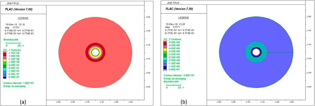
Figure 16. Contour of (a) radial stress and (b) tangential stress at equilibrium state (verification model).

Figure 17

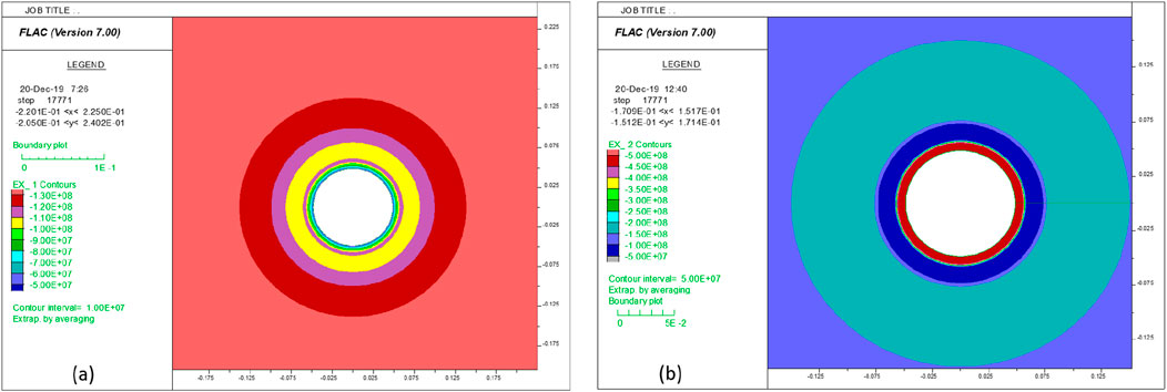
Figure 17. Contour of (a) radial stress and (b) tangential stress at the equilibrium state—a close-up view (verification model).

The simulation result shows that the radial stress on the interface between the liner layer and cement layers (${\mathit{P}}_{\mathit{l}\mathit{c}}$) and the stress on the interface between the cement layer and the formation layer (${\mathit{P}}_{\mathit{c}\mathit{f}}$) are:

${\mathit{P}}_{\mathit{l}\mathit{c}-\mathit{n}\mathit{u}\mathit{m}}=112.4\text{\hspace{0.17em}MPa},$

${\mathit{P}}_{\mathit{c}\mathit{f}-\mathit{n}\mathit{u}\mathit{m}}=105.6\text{\hspace{0.17em}MPa}.$

Because both the layers and loading conditions are axisymmetric, the stresses on the interfaces between layers are the same everywhere along the same interface. A comparison with their corresponding analytical solutions indicates that the differences between the numerical and analytical solutions are trivial at both locations. For example, at the interface between the liner and cement layers, the difference is less than 2%; at the interface between the cement and formation layers, the difference is less than 0.3%.

It may be concluded that the resolution of the selected computational mesh is sufficiently fine to capture the mechanical responses of this three-layered system, including the mechanical behaviors of each layer and the interactions among them.

3.2 Investigative studies

The model validated above may be used to study the liner integrity under various engineering scenarios. Compared with the verification model above, in this model the liner, cement, and formation are modeled as Mohr–Coulomb type elastoplastic materials; the stresses and pressures expected in the field condition are applied on the outer and inner surfaces. The wellbore radius (and outer radius of cement layer) is 7.46 cm; the inner radius of the cement layer (and outer radius of liner) is 5.72 cm; the inner radius of the liner is 4.86 cm. The radius of the outer boundary is set to 20 times the wellbore radius, that is, 1.39 m. The computational mesh has 80 elements in the radial direction and 120 elements in the circumferential direction.

It should be noted that liner-cement and cement–formation interfaces may be modeled as tightly bonded interfaces, or unbonded contacts with limited strength defined by the cohesive strength, frictional angle, and dilation angle; the strength properties can be constant or evolve with the development of plastic deformation (i.e., the strain-hardening or -softening behaviors may be implemented using FLAC’s built-in language, FISH).

3.2.1 Model initialization

To capture the loading effects of the wellbore drilling and completion on the liner, the model is initialized over two steps. In the first step, the model is built without liner and cement layers (see Figure 18); the in situ stresses and pore pressure are initialized; the vertical stress ${\sigma }_V$ ($117$ MPa) and the maximum horizontal stress ${\sigma }_H$ ($138$ MPa) are applied in the y and x directions on the outer boundary; the wellbore fluid pressure $P_w$ ($47.8$ MPa) is applied inside the borehole. Figures 19, 20 display the contours of SXX, SYY, SRR, and STT at the equilibrium state. In the second step, the boundary condition inside the borehole is removed; the layers of cement and liner are generated; the stresses inside the cement layer are initialized to $47.8$ MPa; the borehole pressure of $47.8$ MPa is applied on the inner boundary of the liner. Figure 21 shows the radial stress (SRR) and tangential stress (STT) after the model is solved to equilibrium.

Figure 18

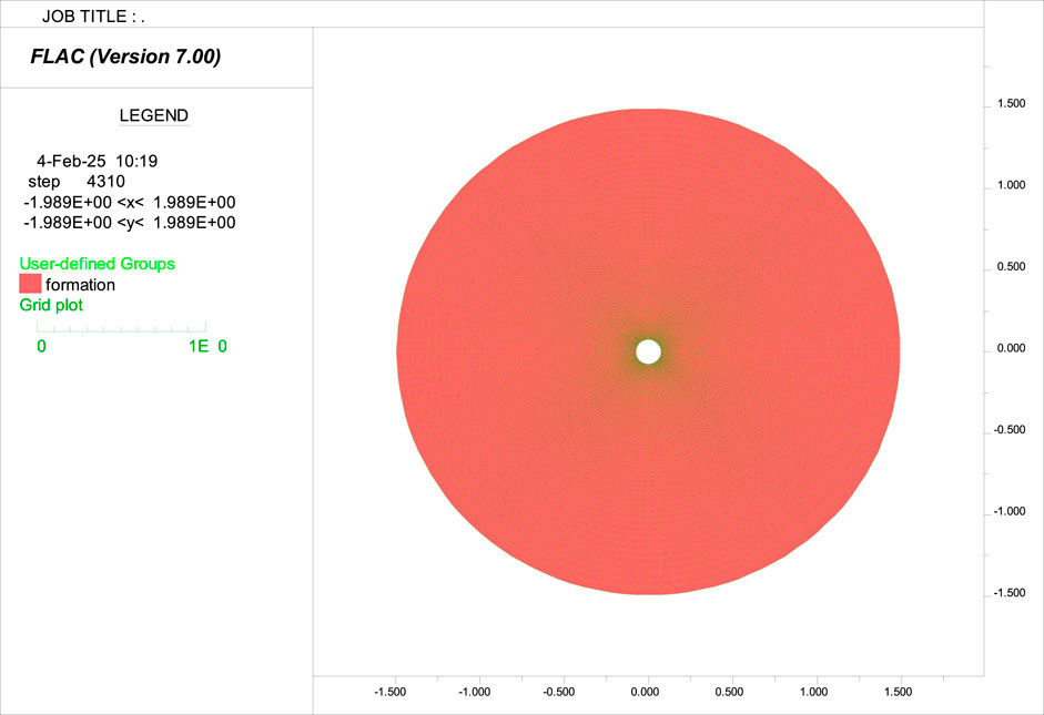
Figure 18. Computational mesh of the liner–cement–formation model without liner and cement layers.

Figure 19

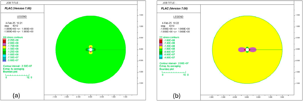
Figure 19. Contour of (a) SXX and (b) SYY in the formation layer before cementing.

Figure 20

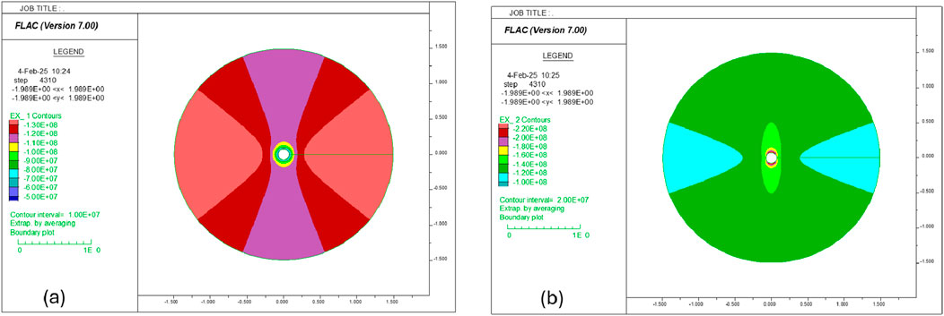
Figure 20. Contour of (a) SRR and (b) STT in the formation layer before cementing.

Figure 21

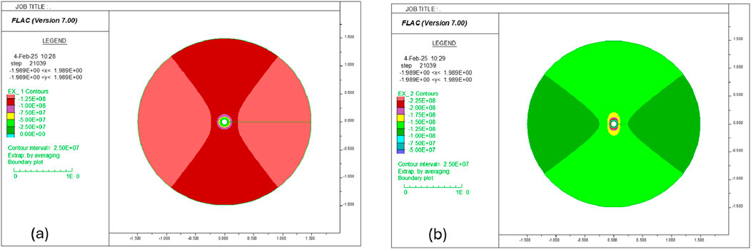
Figure 21. Contour of (a) SRR and (b) STT in the formation layer after cementing.

3.2.2 Investigating effects of voids

Extensive cavities may naturally exist in carbonate formations (Zhang et al., 2019). A poor-quality cementing job may also result in some voids in the cement layer. Considering the gravity effect, in horizontal wells, the upper part of the cement layer is more likely to contain extensive voids. The cavities and voids may hydraulically communicate with the hydraulic fractures through natural fractures or interlayer interfaces.

In the simulations below, we investigate two scenarios, as illustrated in Figure 22. In the first scenario, the major upper part of the cement layer is assumed to be filled with voids. In the second scenario, the upper part of the cement layer contains two cavitated zones, and they do not communicate with each other.

Figure 22

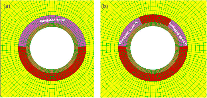
Figure 22. Investigated void scenarios: (a) a single cavitated zone with voids and (b) two cavitated zones with voids.

If there are fluid communication channels between a cavitated zone and hydraulic fractures (HF) (Wang et al., 2022), the maximum fluid pressure inside the voids should be close to the fluid pressure in the hydraulic fractures. If a zone with voids is isolated, its pressure is most likely close to the formation pressure. The size of cavitated zones also has an influence on the load development on the liner. Accordingly, the following four cases are investigated.

Case 1: The cavitated zone in Figure 22a takes formation pressure.

Case 2: The cavitated zone in Figure 22a takes HF pressure.

Case 3: The cavitated zones in Figure 22b take HF pressure in zone A and formation pressure in zone B.

Case 4: The cavitated zones in Figure 22b take HF pressure in zone A and formation pressure in zone B; the zones are smaller.

In the model, the change of the fluid pressure inside the cavitated zones can be simulated by directly adjusting the pore pressure in them. Alternatively, an easier modeling approach is to excavate the cavitated zones and then apply pressures on the boundaries of the excavated holes. These two approaches are equivalent. The second approach is used in this study.

Simulations indicate that, if the upper part of the cement layer is a single cavitated zone, the model can reach equilibrium, and there is no plastic yielding taking place in the liner. The contours of radial and tangential stress are presented in Figure 23 for the cavitated zone with a fluid pressure of 67.7 MPa and in Figures 24b, 25a for the cavitated zone with a fluid pressure of 138 MPa, which corresponds to the peak fracturing pressure during hydraulic fracturing operation. Note that the stress perturbation is expected to occur near the hydraulic fractures during a hydraulic fracturing operation. It will have a non-negligible effect on the fracture propagation and natural fracture reactivation. However, for the borehole segments outside of the fractured borehole segment (which is the target of this study), the perturbation should have only a negligible influence (per Saint-Venant’s principle), so it should be sufficiently conservative to only take the peak pressure in the hydraulic fracturing and impose it inside the cavities. Figures 24a, 25b provide the displacement vectors in the system at an equilibrium state. The magnitude of the maximum displacement vector is higher in the case with higher fluid pressure in the voids, but it is still only approximately 0.6 mm.

Figure 23

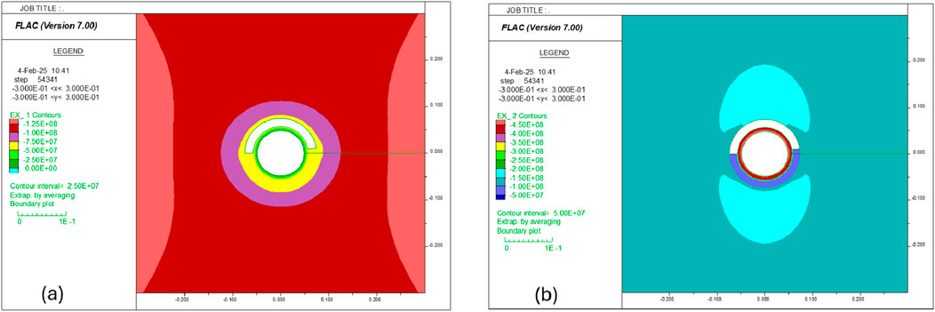
Figure 23. Contour of (a) SRR and (b) STT in Case 1: fluid pressure in voids is 66.7 MPa.

Figure 24

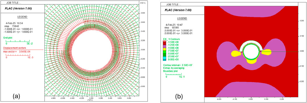
Figure 24. (a) Displacement vectors in Case 1: fluid pressure in voids is 66.7 MPa; (b) contour of SRR in Case 2: fluid pressure in voids is 138 MPa.

Figure 25

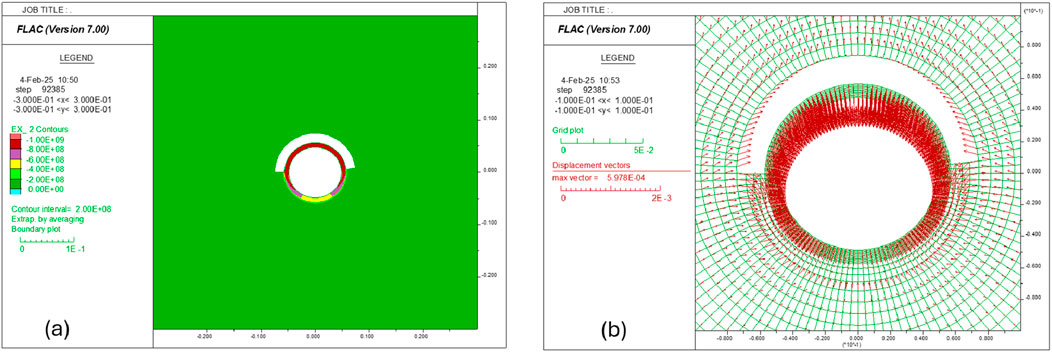
Figure 25. (a) Contour of STT and (b) displacement vectors in Case 2: fluid pressure in voids is 138 MPa.

Simulations show that the model cannot reach equilibrium in Case 3, where zone A has a fluid pressure of 138 MPa and zone B has a fluid pressure of 67.7 MPa. As shown in Figure 26a, the liner starts to yield plastically when the pressure in zone A reaches 130 MPa. If we keep increasing the pressure inside zone A, then fix it at 138 MPa after it reaches that magnitude but continue the simulation, the liner is observed to lose its integrity, as shown in Figures 26b–28a. Figures 26b, 27a present the distributions of radial and tangential stresses in the system when the maximum displacement on the liner reaches 1.88 cm (see Figure 27b). Figure 28a shows the corresponding plastic state in the system. Interestingly, the deformation and plastic patterns in this case look similar to those in the stand-alone liner with non-uniform loading conditions, for example, comparing Figure 12 with Figures 27, 28. However, this is actually as expected because the load distribution patterns on the liner are very similar in these two cases.

Figure 26

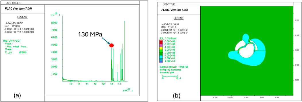
Figure 26. (a) Collapse pressure of the liner and (b) the contour of SRR in Case 3, where the fluid pressure is 138 MPa in zone A and 66.7 MPa in zone B.

Figure 27

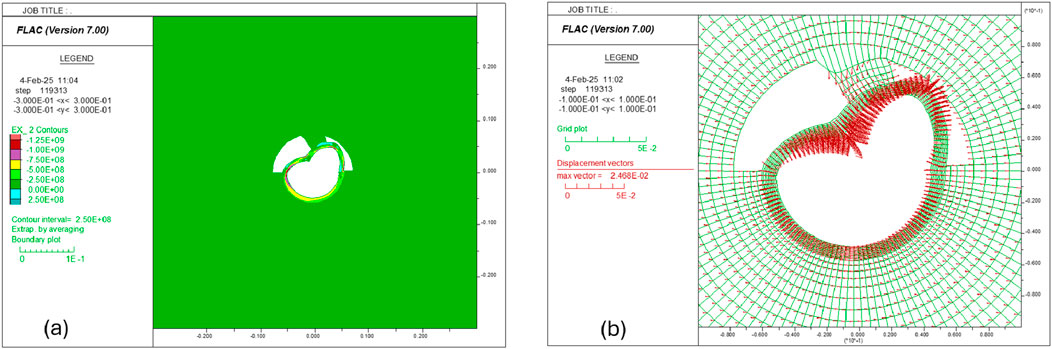
Figure 27. (a) Contour of STT and (b) displacement vectors in Case 3, where the fluid pressure is 138 MPa in zone A and 66.7 MPa in zone B.

Figure 28

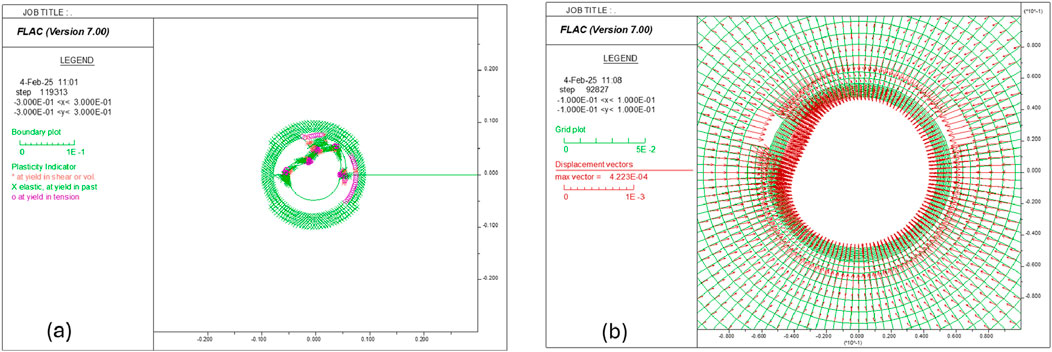
Figure 28. (a) Plastic state in Case 3, where the fluid pressure is 138 MPa in zone A and 66.7 MPa in zone B; (b) displacement vectors in Case 4, where the fluid pressure is 138 MPa in zone A and 66.7 MPa in zone B; the zones are smaller than in Case 3.

In Case 4, the extensions of two cavitated zones (in Case 3) are arbitrarily reduced, as shown in Figures 28b–29. The simulations report that the model can reach equilibrium, and there is no plastic yielding developed in the liner. At the equilibrium state, the maximum deformation on the liner is less than 0.5 mm (see Figure 28b). The radial and tangential stress contours at the equilibrium state are displayed in Figure 29.

Figure 29

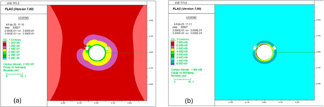
Figure 29. Contour of (a) SRR and (b) STT in Case 4, where the fluid pressure is 138 MPa in zone A and 66.7 MPa in zone B; the zones are smaller than in Case 3.

It should be noted that the extension, shape, and location of imperfections (cavities, vugs, and fractures) in the formation and cement will have a significant impact on the magnitude and distribution of stress on the liner. For example, cavities that are smaller and farther from the liner will have a reduced impact. In the scenarios investigated above, the cavities are chosen arbitrarily. Because the field data are lacking, we did not intend to make predictions for a real case but rather to provide a generic demonstration.

4 Conclusion

Large deformation and/or failure of the liner are often experienced during hydraulic fracturing operations in carbonate formations. While it is well understood that liner deformation can be caused by many mechanisms, this work explored the possibility of a poor quality cementing job and cavities in the formation causing liner deformation and failure through extensive numerical simulations.

We built both stand-alone liner models and liner–cement–formation interaction models. The stand-alone liner models showed that, if the loads are distributed uniformly inside and outside of the liner in the radial direction, the liner can retain its integrity in both burst and collapse modes. However, the collapse pressure can drop sharply if the distribution of the load on the outer boundary becomes non-uniform. The collapse pressure can decrease further if the confinement is removed. The liner–cement–formation models showed that, if the cement or the formation contains cavities where the pressure is much higher or lower than the pressure inside the liner during hydraulic fracturing treatment, the liner can deform largely and fail in burst or collapse modes.

The diagnostic models developed in this work can capture the primary behaviors of each component and the response of the liner–cement–formation system. The investigation indicates that the uniformity of load and confinement could be the most critical factors behind large liner deformation experienced during hydraulic fracturing operations in carbonate formations. The model developed in this work can be further refined to accommodate other factors and procedures when applied to support a specific hydraulic fracturing job. To generalize the findings in this study, more systematic parametric studies should be performed to study the liner stressing and integrity to the varying void size, distance, and cement strength.

It should be noted that the model predictions in this work are based on several assumptions and simplifications. The mechanical properties responses of the liner are calibrated on its burst pressure and yield pressure loading mode; both are uniform and axisymmetric. Its reliability and accuracy in predicting the deformation and loading capacity of the liner under non-uniform loading conditions must be validated with laboratory data of crushing liners under non-uniform loading conditions. If there is a significant discrepancy between the model prediction and the laboratory measurement, the liner model and properties must be further calibrated, and all the simulations in the work must be re-run to refine the analysis results. In the liner–cement–formation models, the fractured borehole segment is assumed to be horizontal and drilled in the minimum horizontal stress direction to simplify the model setup. The operational procedures should have a non-negligible influence on the load development on the liner, but they were only approximately simulated in this work. In addition, the effects of the fluid diffusion, thermal–mechanical interaction, and hydro-mechanical interaction were not considered. In many practical situations, the three-dimensional stress effect may have an important influence on the force development and distribution on the liner. All these factors should be accommodated if the developed models are adopted as an accurate predictive tool, for example, to optimize the injection pressure that can prevent plastic yielding and collapse of the liner during HF stimulation.

Data availability statement

The raw data supporting the conclusions of this article will be made available by the authors, without undue reservation.

Author contributions

YH: Writing – original draft, Project administration, Writing – review and editing, Funding acquisition, Formal Analysis, Supervision, Methodology, Investigation, Data curation, Software, Visualization, Conceptualization, Validation, Resources. DP: Writing – review and editing, Funding acquisition, Resources, Writing – original draft, Visualization, Software, Formal Analysis, Validation, Conceptualization, Data curation, Investigation, Supervision, Methodology, Project administration. YA: Software, Supervision, Funding acquisition, Formal Analysis, Writing – review and editing, Resources, Conceptualization, Project administration, Writing – original draft, Methodology, Data curation, Validation, Visualization, Investigation. KR: Funding acquisition, Resources, Visualization, Writing – original draft, Validation, Formal Analysis, Project administration, Writing – review and editing, Conceptualization, Investigation, Data curation, Supervision, Methodology, Software.

Funding

The authors declare that no financial support was received for the research and/or publication of this article.

Conflict of interest

Author KR was employed by the Saudi Arabian Oil Co., Authors YH, DP and YA were employed by Aramco Americas.

Generative AI statement

The authors declare that no Generative AI was used in the creation of this manuscript.

Any alternative text (alt text) provided alongside figures in this article has been generated by Frontiers with the support of artificial intelligence and reasonable efforts have been made to ensure accuracy, including review by the authors wherever possible. If you identify any issues, please contact us.

Publisher’s note

All claims expressed in this article are solely those of the authors and do not necessarily represent those of their affiliated organizations, or those of the publisher, the editors and the reviewers. Any product that may be evaluated in this article, or claim that may be made by its manufacturer, is not guaranteed or endorsed by the publisher.

References

De Andrade, J., and Sangesland, S. (2016). Cement sheath failure mechanisms: numerical estimates to design for long-term well integrity. J. Petroleum Sci. Eng. 147, 682–698. doi:10.1016/j.petrol.2016.08.032

CrossRef Full Text | Google Scholar

Dusseault, M. B., Bruno, M. S., and Barrera, J. (2001). Casing shear: causes, cases, cures. SPE Drill. and Complet. 16 (02), 98–107. doi:10.2118/72060-pa

CrossRef Full Text | Google Scholar

Furui, K., Fuh, G. F., Abdelmalek, N. A., and Morita, N. (2010). A comprehensive modeling analysis of borehole stability and production-liner deformation for inclined/horizontal wells completed in a highly compacting chalk formation. SPE Drill. and Complet. 25 (04), 530–543. doi:10.2118/123651-pa

CrossRef Full Text | Google Scholar

Guo, B., Shan, L., Jiang, S., Li, G., and Lee, J. (2018). The maximum permissible fracturing pressure in shale gas wells for wellbore cement sheath integrity. J. Nat. Gas Sci. Eng. 56, 324–332. doi:10.1016/j.jngse.2018.06.012

CrossRef Full Text | Google Scholar

Han, Y., Tallin, A. G., and Wong, G. K. (2015). “Impact of depletion on integrity of sand screen in depleted unconsolidated sandstone formation,” in 49th US rock mechanics/geomechanics symposium (American Rock Mechanics Association).

Google Scholar

Han, Y., Abousleiman, Y. N., and Alruwaili, K. M. M. (2022). Calibration and simulation of a wellbore liner. U.S. Patent No. 11,270,048. Washington, DC: U.S. Patent and Trademark Office.

Google Scholar

Han, Y., Phan, D., and AlRuwaili, K. (2024). Hybrid procedure for evaluating stress magnitude and distribution on a liner. U.S. Patent No. 11,940,592. Washington, DC: U.S. Patent and Trademark Office.

Google Scholar

ITASCA (2011). Fast lagrangian analysis of continua, version 7.0. Minneapolis, Minnesota: ITASCA.

Google Scholar

Kiran, R., Teodoriu, C., Dadmohammadi, Y., Nygaard, R., Wood, D., Mokhtari, M., et al. (2017). Identification and evaluation of well integrity and causes of failure of well integrity barriers (A review). J. Nat. Gas Sci. Eng. 45, 511–526. doi:10.1016/j.jngse.2017.05.009

CrossRef Full Text | Google Scholar

Li, Q., Zhao, D., Yin, J., Zhou, X., Li, Y., Chi, P., et al. (2023). Sediment instability caused by gas production from hydrate-bearing sediment in northern South China Sea by horizontal wellbore: evolution and mechanism. Nat. Resour. Res. 32 (4), 1595–1620. doi:10.1007/s11053-023-10202-7

CrossRef Full Text | Google Scholar

Li, Q., Liu, J., Wang, S., Guo, Y., Han, X., Li, Q., et al. (2024). Numerical insights into factors affecting collapse behavior of horizontal wellbore in clayey silt hydrate-bearing sediments and the accompanying control strategy. Ocean. Eng. 297, 117029. doi:10.1016/j.oceaneng.2024.117029

CrossRef Full Text | Google Scholar

Liu, B., and Han, Y. (2005). The theory, example and application guide of FLAC. China: China Communications Press.

Google Scholar

Montgomery, C. T., and Smith, M. B. (2010). Hydraulic fracturing: history of an enduring technology. J. Petroleum Technol. 62 (12), 26–40. doi:10.2118/1210-0026-jpt

CrossRef Full Text | Google Scholar

Moska, R., Labus, K., and Kasza, P. (2021). Hydraulic fracturing in enhanced geothermal systems—field, tectonic and rock mechanics conditions—a review. Energies 14 (18), 5725. doi:10.3390/en14185725

CrossRef Full Text | Google Scholar

Mou, Y., Zhao, H., Cui, J., Wang, Z., Wei, F., and Han, L. (2023). Failure analysis of casing in shale oil Wells under multistage fracturing conditions. Processes 11 (8), 2250. doi:10.3390/pr11082250

CrossRef Full Text | Google Scholar

Peng, S., Fu, J., and Zhang, J. (2007). Borehole casing failure analysis in unconsolidated formations: a case study. J. Petroleum Sci. Eng. 59 (3-4), 226–238. doi:10.1016/j.petrol.2007.04.010

CrossRef Full Text | Google Scholar

Shi, Z., Zhang, T., and Xiang, H. (2007). Exact solutions of heterogeneous elastic hollow cylinders. Compos. Struct. 79 (1), 140–147. doi:10.1016/j.compstruct.2005.11.058

CrossRef Full Text | Google Scholar

Vudovich, A., Chin, L. V., and Morgan, D. R. (1988). “Casing deformation in Ekofisk,” in Offshore technology conference.

Google Scholar

Wang, W., and Taleghani, A. D. (2014). Three-dimensional analysis of cement sheath integrity around wellbores. J. Petroleum Sci. Eng. 121, 38–51. doi:10.1016/j.petrol.2014.05.024

CrossRef Full Text | Google Scholar

Wang, T., Zhou, W., Chen, J., Xiao, X., Li, Y., and Zhao, X. (2014). Simulation of hydraulic fracturing using particle flow method and application in a coal mine. Int. J. Coal Geol. 121, 1–13. doi:10.1016/j.coal.2013.10.012

CrossRef Full Text | Google Scholar

Wang, L., Wu, X., Hou, L., Guo, Y., Bi, Z., and Yang, H. (2022). Experimental and numerical investigation on the interaction between hydraulic fractures and vugs in fracture-cavity carbonate reservoirs. Energies 15 (20), 7661. doi:10.3390/en15207661

CrossRef Full Text | Google Scholar

Waters, G., Dean, B., Downie, R., Kerrihard, K., Austbo, L., and McPherson, B. (2009). “Simultaneous hydraulic fracturing of adjacent horizontal wells in the Woodford Shale,” in SPE hydraulic fracturing technology conference and exhibition (SPE database Onepetro.org), 119635.

Google Scholar

Wilson, W. N., Perkins, T. K., and Striegler, J. H. (1979). “Axial buckling stability of cemented pipe,” in SPE annual technical conference and exhibition (SPE database Onepetro.org).

Google Scholar

Yousuf, N., Olayiwola, O., Guo, B., and Liu, N. (2021). A comprehensive review on the loss of wellbore integrity due to cement failure and available remedial methods. J. Petroleum Sci. Eng. 207, 109123. doi:10.1016/j.petrol.2021.109123

CrossRef Full Text | Google Scholar

Zhang, F., An, M., Yan, B., Wang, Y., and Han, Y. (2019). A novel hydro-mechanical coupled analysis for the fractured vuggy carbonate reservoirs. Comput. Geotechnics 106, 68–82. doi:10.1016/j.compgeo.2018.10.013

CrossRef Full Text | Google Scholar