Improved design of passive wireless sensor for ultra-high temperature environment and its back-end circuit measurement system

Introduction: An improved passive wireless sensor is presented for ultra-high temperature environments, utilizing a folded Complementary Split-Ring Resonator (CSRR) structure. A dedicated back-end circuit measurement system is also developed to support the improved sensor.

Methods: The sensor design was optimized with an aluminum nitride ceramic substrate and a platinum layer, incorporating distributed compensation to enhance thermal stability. A matching back-end circuit measurement system was designed for high-sensitivity signal reception and processing.

Results: Performance testing showed that at 1,000 °C, the quality factor was increased from 241 to 418, and the sensitivity was raised from 10.89 to 17.12. The temperature coefficient of frequency was significantly improved from –14.23 ppm/°C to –3.76 ppm/°C, demonstrating superior stability. Measurements showed that the back-end system achieved a mere 0.02 GHz error in resonant frequency compared to a network analyzer, with a total test error below 1%.

Discussion: The proposed sensor effectively minimizes performance degradation at high temperatures, achieving high-accuracy and stable wireless signal detection. This work provides a reliable passive sensing solution for real-time monitoring in ultra-high temperature conditions.

1 Introduction

With the rapid development of industrial automation, aerospace, energy and other fields, as well as the rise of digital twin technology, the demand for real-time monitoring of sensors in ultra-high temperature environments has been increasing (Dawn et al., 2024). Traditional contact thermocouples are difficult to serve for a long time due to lead aging, insulation failure, and electromagnetic interference. However, active wireless sensors cannot meet application requirements due to the rapid degradation of battery or energy harvesting module performance under ultra-high temperature conditions (Swarna and Kolluru, 2024). Passive wireless sensors have become a key technology for solving this problem due to their no external power supply, high temperature resistance, simple structure, and wireless signal transmission (Grosinger and Michalowska-Forsyth, 2022). However, existing passive wireless high-temperature sensors still have shortcomings in sensitivity, stability, and measurement range, and their performance needs to be improved through structural optimization and material improvement (Bandewad et al., 2023). Among numerous passive wireless sensing architectures, the Complementary Split-Ring Resonator (CSRR) is an efficient electromagnetic resonance structure, which is widely used in passive wireless sensors due to its unique frequency response characteristics and compact size (Kumar and Madhan, 2025).

Haq and Koziel proposed a fast optimization design and parameter adjustment method for microwave sensors based on CSRR. This method established an inverse proxy model and combined pre-optimized data to lock in frequency and improve Q-value. The results showed that the quality factor of the optimized sensor was significantly improved, and the inverse regression model could accurately invert the dielectric constant of the material (Haq and Koziel, 2022). Jiang et al. built a high-sensitivity microwave microfluidic sensor based on CSRR and forked electrodes. By optimizing the outer ring structure and utilizing a plastic microfluidic cavity with high-electric field strength to enhance electric field confinement, the measurement sensitivity of liquid complex dielectric constant was improved. The average sensitivity was 1.23%, which was superior to similar sensors (Jiang et al., 2023). Xiao et al. designed a compact planar sensor based on dual-band CSRR for synchronously measuring the microwave and dielectric properties of solid materials. This method utilized coplanar waveguides and waveguide probes to excite separately, achieving dual-scale independent detection with small sample sizes. The results showed that the sensor exhibited high-sensitivity (Xiao et al., 2022). Prakash and Gupta proposed a high-sensitivity chemical sensor based on groove type CSRR. Integrating hollow tube structures in high-field strength areas simplified the placement requirements of the liquid sample to be tested. This method utilized a composite left-right transmission line to excite and increase the width of the capacitor gap, improving electromagnetic coupling efficiency and sensitivity. It was found that the sensor had low-cost and real-time detection (Prakash and Gupta, 2022). Buragohain et al. proposed a low-cost microwave sensor based on a double split CSRR structure to meet the high-precision detection requirements of liquid dielectric constant. This method enhanced electric field coupling by designing orthogonal slit structures on the substrate, and utilized the principle of equivalent circuits to achieve efficient excitation in frequency bands. The results indicated that the measured error of the sensor was less than 5% (Buragohain et al., 2023). Han et al. built a highly integrated microwave microfluidic sensor based on hexagonal CSRR and substrate integrated waveguide structure. This method enhanced electric field constraint through metal via rings, combined microfluidic channels to achieve ultra-low sample size detection, and established a feature matrix model to analyze dielectric parameters. The results showed that the sensitivity of the sensor was 0.448% (Han et al., 2024). Das et al. proposed an anti-interference microwave sensor based on differential CSRR structure to address the susceptibility of liquid dielectric constant measurement to environmental interference. This method optimized the frequency band resonators and utilized the principle of differential measurement to eliminate the influence of environmental noise. The sensor could achieve high sensitivity detection on the substrate (Das et al., 2024). Vaidya et al. designed a novel compact RF sensor based on CSRR for detecting impurities in liquid samples. The sensor optimized the field distribution through a curved structure design and used changes in dielectric constant to measure impurity levels in ordinary liquids. The monitoring sensitivity of the sensor reached 39.36% (Vaidya et al., 2025). Zegadi et al. proposed a high-Q microstrip sensor based on offset CSRR structure to meet the high-precision dielectric detection requirements. This method enhanced field constraints through asymmetric microstrip feeding and resonator offset design, achieving high-resolution detection. The results showed that the sensor exhibited the minimum error measurement at a bandwidth of 330 MHz (Zegadi et al., 2025).

Numerous scholars conducting research on the sensor design of CSRR structures and achieving good results. However, in ultra-high temperature environments, the electromagnetic parameters of CSRR structures are still susceptible to temperature effects, leading to a decrease in sensor performance. Therefore, the research improves the passive wireless sensor in ultra-high temperature environments. A new sensor scheme based on CSRR structure optimization is proposed, and the supporting back-end circuit measurement system is designed. The research aims to enhance the stability, sensitivity, and measurement accuracy of the sensor under extreme temperature conditions, while achieving efficient and reliable passive wireless signal transmission and detection.

The innovation of the research lies in:

• Proposing a novel resonant structure based on folded CSRR, which suppresses frequency drift in ultra-high temperature environments through distributed compensation units and bending angle optimization.

• Designing a back-end circuit measurement system for the improved passive wireless high-temperature sensor matching to achieve passive wireless excitation, high-sensitivity reception, and high-precision demodulation of microwave signals.

2 Methods and materials

Firstly, an improved design method for passive wireless high-temperature sensors based on CSRR structure is built to enhance the performance of the sensor in ultra-high temperature environments. Then, the back-end circuit measurement system is designed to achieve high-sensitivity reception of microwave signals.

2.1 Material selection and electromagnetic parameter measurement of passive wireless high-temperature sensors

The performance of passive wireless sensors in ultra-high temperature environments highly depends on the selected materials and the precise measurement of their electromagnetic parameters. The study selects aluminum nitride ceramics as the substrate material, which has high thermal conductivity, low dielectric loss, and excellent high-temperature stability (Gu et al., 2022). The resonant structure adopts a platinum metal layer, which has strong oxidation resistance and small changes in conductivity at high temperatures, and has good processing performance. The transmission method and scattering parameter method, as the core methods for electromagnetic parameter measurement, can accurately characterize the dielectric properties of materials in the microwave frequency band (Ma et al., 2022). Therefore, the study adopts these two methods to systematically measure key material parameters. The study employs the transmission line theory. The complex dielectric constant is calculated through transmission coefficients to explore the dielectric properties of materials in the microwave frequency band. The expression is shown in Equation 1.

$\epsilon ={\left(\left(c·\ln \left(1-\left|S_{21}\right|\right)\right)/\left(j\omega d\right)\right)}^2(1)$

In Equation 1, $\epsilon$ represents the complex dielectric constant. $\left|S_{21}\right|$ represents the transmission coefficient. $c$ and $\omega$ respectively represent the propagation velocity (m/s) and angular frequency (rad/s) of electromagnetic waves in vacuum. $j$ and $d$ represent imaginary units and sample thickness (m), respectively. The relationship between reflection coefficient and impedance is crucial for analyzing material properties in scattering parameter measurement. The research takes a network analyzer to measure reflection coefficients and establishes the relationship between materials and features, as shown in Equation 2 (Han et al., 2022).

$\left|S_{11}\right|=\left(Z_{in}-Z_0\right)/\left(Z_{in}+Z_0\right)(2)$

In Equation 2, $\left|S_{11}\right|$ signifies the reflection coefficient. The magnitude of the reflection coefficient is between [0,1], and 0< $\left|S_{11}\right|$ <1. $Z_{in}$ and $Z_0$ represent the input impedance (Ω) and characteristic impedance (Ω), respectively. The material loss characteristics are quantitatively characterized. The quantitative relationship between resonance frequency shift and dielectric constant change is established to achieve temperature characteristic analysis of CRSS structures, as shown in Equation 3.

$\left\{\begin{array}{l}\tan \delta ={\epsilon }^{″}/{\epsilon }^{\prime }\\ \Delta f_r=\frac{f_r}{2}·\frac{\Delta {\epsilon }^{\prime }}{{\epsilon }^{\prime }}\end{array}\right.(3)$

In Equation 3, $\tan \delta$ represents the loss tangent. ${\epsilon }^{″}$ and ${\epsilon }^{\prime }$ represent the imaginary and real parts of the complex dielectric constant, respectively, reflecting energy dissipation and polarization ability. $\Delta f_r$ represents the resonant frequency offset (Hz). $f_r$ represents the resonant frequency. $\Delta {\epsilon }^{\prime }$ represents the change in the real part of the dielectric constant. To optimize sensor design, the electromagnetic coupling efficiency is accurately calculated and the resonator performance is evaluated through quality factor, as shown in Equation 4 (Li et al., 2024).

$\left\{\begin{array}{l}Q=f_r/\text{FWHM}\\ \eta =1-{\left|S_{11}\right|}^2-{\left|S_{21}\right|}^2\end{array}\right.(4)$

In Equation 4, $Q$ signifies the quality factor. A higher quality factor value indicates a sharper resonance peak, which translates to lower energy loss per cycle and higher frequency selectivity. This is crucial for the resolution and stability of sensors, especially in high-temperature environments where losses may increase. $\text{FWHM}$ represents the bandwidth of the resonance curve at half the peak. $\eta$ represents the electromagnetic coupling efficiency. This quantity directly influences the readability of the sensor. Higher coupling efficiency means a stronger sensor response signal for a given incident power, improving the signal-to-noise ratio and the maximum interrogation distance. Optimizing the sensor design, including the folded CSRR structure and the matching with the substrate-integrated waveguide, aims to maximize this efficiency. In high-temperature environments, frequency stability is crucial. It is evaluated by the temperature coefficient of the resonant frequency, as shown in Equation 5 (Nagmani and Behera, 2024).

$\alpha T_f=\frac{1}{f_r}·\frac{\mathrm{\partial }{f}_r}{\mathrm{\partial }{T}_e}(5)$

In Equation 5, $\alpha T_f$ represents the frequency temperature coefficient. $T_e$ represents the ambient temperature. The schematic diagram of the transmission method and scattering parameter signal flow is shown in Figure 1.

Figure 1

Figure 1. Schematic diagram of transmission method and scattering parameter signal flow. (a) Schematic diagram of transmission method. (b) Scattering parameter signal flow.

Figure 1a shows the transmission method model. Electromagnetic waves enter from Port 1 and exit from Port 2 after passing through the sample, reflecting the transmission process of electromagnetic waves in the medium. Scattering parameters describe the signal reflection and transmission between ports in a system characterized by a specific reference characteristic impedance. This parameter measures the degree of mismatch between the input impedance and the system reference characteristic impedance. Figure 1b shows the scattering parameter signal flow, describing the energy transfer and reflection relationship between the transmission coefficient and reflection coefficient among ports. It reflects the influence of the sample on the propagation characteristics of electromagnetic waves. The scattering parameter signal can be directly associated with the power flow. The square of the amplitude of the incident wave and the amplitude of the reflected wave are proportional to the incident power and reflected power of the corresponding port, respectively. Its representation is shown in Equation 6.

$\left\{\begin{array}{l}{b}_1=\left|S_{11}\right|a_1+\left|S_{12}\right|a_2\\ b_2=\left|S_{21}\right|a_1+\left|S_{22}\right|a_2\\ T_p=P_{\text{trans}}/P_{\text{incident}}={\left|S_{21}\right|}^2\\ {\mathrm{\Gamma }}_p=P_{\text{reflect}}/P_{\text{incident}}={\left|S_{11}\right|}^2\end{array}\right.(6)$

In Equation 6, $a_1$ and $a_2$ represent the amplitude of the incident wave. $b_1$ and $b_2$ represent the amplitude of the reflected wave. $\left|S_{12}\right|$ represents the forward transmission coefficient. $\left|S_{22}\right|$ represents the coefficient of retroreflection. $T_p$ represents the power transmission coefficient. ${\mathrm{\Gamma }}_p$ represents the power reflection coefficient. $P_{\text{incident}}$ represents the power incident on port 1. $P_{\text{trans}}$ represents the power transmitted from port 1 to port 2. $P_{\text{reflect}}$ represents the power reflected back from port 1.

2.2 Design of passive wireless high temperature sensor based on CSRR structure

After completing material selection and electromagnetic parameter measurement, the study further optimizes the sensor based on CSRR structure through High Frequency Structure Simulator (HFSS) (Shinde et al., 2024). A passive wireless high-temperature sensor based on folded CSRR and substrate integrated waveguide is proposed to enhance the performance of the sensor. To solve the high-temperature frequency deviation in traditional CSRR, a resonant frequency model of the folded structure is first built. The influence of the folding angle on the propagation path of electromagnetic waves is analyzed. And adopt the effective dielectric constant to explain the influence of non-uniform media on the electromagnetic wave propagation characteristics within the sensor structure. For the proposed folded CSRR structure, which is fundamentally based on a planar resonator fabricated on a substrate, the effective dielectric constant was calculated using the well-established analytical expression for a microstrip line. The calculation of resonance frequency and effective dielectric constant is shown in Equation 7.

$\left\{\begin{array}{l}{f}_r^{\prime }=\frac{c}{4L_{eff}\sqrt{{\epsilon }_{eff}}}·\frac{1}{1+\frac{1}{2}\left(1-\cos \theta \right)}\\ {\epsilon }_{eff}=\frac{{\epsilon }_r+1}{2}+\frac{{\epsilon }_r-1}{2}·\frac{1}{\sqrt{1+12\frac{H}{W}}}\end{array}\right.(7)$

In Equation 7, $f_r^{\prime }$ signifies the resonant frequency (Hz) of the folded structure. $L_{eff}$ signifies the effective path length (m). ${\epsilon }_{eff}$ represents the effective dielectric constant. $\theta$ represents the folding angle. ${\epsilon }_r$ represents the relative dielectric constant of the substrate material (the relative dielectric constant of aluminum nitride is about 8.8). $H$ represents the thickness of the substrate. $W$ represents the width of the conduction band. To achieve wide temperature range stability, distributed compensation units are designed at each bend of the folding structure, and their resonant frequency expression is shown in Equation 8.

$f_r^{″}=f_r^{\prime }·\underset{i=1}{\overset{n}{\mathrm{\Pi }}}\left[1+{\beta }_i\left(T-T_0\right)\right](8)$

In Equation 8, $f_r^{″}$ represents the compensated resonant frequency (Hz). ${\beta }_i$ signifies the temperature coefficient of the $i$-th compensation unit. $T_0$ signifies the reference temperature. $n$ signifies the total number of compensation units. Then, the study comprehensively considers the quality factors of each component to accurately evaluate the energy loss characteristics, as shown in Equation 9.

$Q_{total}={\left(\frac{1}{Q_{CSRR}}+\frac{1}{Q_{SIW}}\right)}^{-1}+Q_{coup}(9)$

In Equation 9, $Q_{total}$ represents the total quality factor. $Q_{CSRR}$ and $Q_{SIW}$ represent the quality factors of CSRR and substrate integrated waveguide, respectively. $Q_{coup}$ represents the quality factor of the coupled structure. To quantify the sensitivity enhancement effect brought by folding structures, a sensitivity superposition model with multiple hotspot regions is established, as shown in Equation 10 (Yan et al., 2023).

$S={\displaystyle \sum _{k=1}^m}\frac{\mathrm{\partial }{f}_r^{\prime }}{\mathrm{\partial }{\epsilon }_k}·\frac{A_k}{A_{total}}(10)$

In Equation 10, $S$ represents the total sensitivity. $m$ signifies the number of local regions in the folded structure where the electric field is enhanced. $\frac{\mathrm{\partial }{f}_r^{\prime }}{\mathrm{\partial }{\epsilon }_k}$ and $A_k$ respectively represent the sensitivity and equivalent active area (m²) of the $k$-th hotspot region. $A_{total}$ represents the total effective area (m²) of the folded structure. A frequency offset model for multi-physics field coupling is established to comprehensively evaluate performance changes in high-temperature environments, as shown in Equation 11.

$\Delta f=\sqrt{{\left(\Delta f_{thermal}\right)}^2+{\left(\Delta f_{stress}\right)}^2+{\left(\Delta f_{elec}\right)}^2}(11)$

In Equation 11, $\Delta f$ represents the total frequency offset (Hz). $\Delta f_{thermal}$ and $\Delta f_{stress}$ respectively represent thermally induced frequency deviation (Hz) and stress-induced frequency deviation (Hz). $\Delta f_{elec}$ represents the electrical frequency offset (Hz). To ensure the mechanical stability of the stacked structure at high temperatures, a deformation coefficient evaluation index is defined, as shown in Equation 12 (Athar et al., 2023).

$\gamma =\frac{\Delta L/L_0}{\Delta T·\Delta P}(12)$

In Equation 12, $\gamma$ represents the deformation coefficient. $\Delta L$ represents the change in structural length. $L_0$ signifies the length of the original structure. $\Delta P$ signifies the amount of pressure change. The schematic diagram of the passive wireless high-temperature sensor before and after improvement is shown in Figure 2.

Figure 2

Figure 2. Schematic diagram of passive wireless high-temperature sensor before and after improvement. (a) Structure diagram of sensor design before improvement. (b) Structure diagram of sensor design after improvement.

Figure 2a shows the sensor design before improvement, with key dimensional parameters of the sensor labeled, including length, pitch, main gap, first side gap, wiring back width, inner and outer widths, and distance. Figure 2b shows the improved sensor design, which has a more complex structure and adds multiple folding parts to improve the sensor performance. In Figure 2, L represents the base edge length, O_w represents the width of the outer resonant ring, I_w represents the width of the inner resonant ring, F_sg represents the width of the outer resonant ring, M_g represents the width of the inner resonant ring, P represents the distance between adjacent metalized vias, and D represents the diameter of the metalized vias. The initial size of the sensor is determined based on the basic resonance conditions of the target frequency band. The effective electrical length of the resonator was initially estimated based on the guided wave wavelength in the aluminum nitride substrate. The initial values of ring width and gap width are selected from typical CSRR designs reported in literature, and further refined through parameter scanning simulations in HFSS to ensure that fundamental resonance occurs within the desired frequency band. The determination of the final size takes into account the wavelength at the target resonant frequency. The total electrical length of the folded CSRR structure has been optimized and adjusted to reduce physical size while maintaining resonance. Optimized the folding angle and number of folds to achieve the required equivalent path length and electric field distribution. The optimization process adopts HFSS simulation platform, combined with parameterized scanning and iterative optimization. This method identifies sensitive parameters by sequentially changing individual variables and observing their impact on resonance frequency and performance indicators. Then, using the built-in optimizer in HFSS, multiple key variables are adjusted simultaneously to automatically find the optimal size combination that meets all optimization objectives. The optimizer will iterate based on the set objective function.

2.3 Design method of back-end circuit measurement system for improved passive wireless high temperature sensor

After designing the improved passive wireless high-temperature sensor based on CSRR structure, to ensure efficient signal acquisition and processing, and enable the sensor to operate reliably in actual working conditions, a matching back-end circuit measurement system is proposed to achieve stable transmission and high-precision measurement of wireless signals in ultra-high temperature environments. The back-end circuit measurement system for the improved passive wireless high-temperature sensor is displayed in Figure 3.

Figure 3

Figure 3. Schematic diagram of back-end circuit measurement system of improved passive wireless high-temperature sensor.

In Figure 3, the signal source module in the back-end circuit measurement system uses the LMX2595 chip and is configured through an STM32 micro-controller to provide stable high-frequency excitation signals. The power detection module is responsible for detecting the power of the RF signal returned by the sensor, including components such as resistors, enablement, and filters, to accurately measure the signal. To optimize frequency stability, a constant temperature crystal oscillator is taken as a reference clock source. The output frequency of the phase-locked loop chip is calculated, as shown in Equation 13 (Athar et al., 2023).

$f_{out}=\frac{N·f_{ref}}{R}(13)$

In Equation 13, $f_{out}$ represents the output frequency (Hz). $N$ represents the frequency division coefficient. $f_{ref}$ represents the reference frequency. $R$ represents the reference frequency division ratio. The signal source chip structure in the signal source module is shown in Figure 4.

Figure 4

Figure 4. Structure diagram of signal source chip in signal source module.

In Figure 4, the signal source chip is configured through a serial interface and integrates a charge pump, modulator, and N-divider to improve frequency stability and accuracy. The main function of the transmission channel conversion module is to optimize the signal transmission path and reduce reflection loss and noise interference. The study selects low loss RO4350B substrate as the printed circuit board material to ensure signal transmission efficiency (Rahim et al., 2023). This laminate possesses well-characterized high-frequency properties, with a dielectric constant of 3.66, a dissipation factor of 0.0037 at 10 GHz, and a typical thickness of 0.508 mm for the layer used in this design. The conductor thickness is 35 μm. Optimizing the transmission efficiency is the core goal of module design, and its computational model is shown in Equation 14.

${\eta }_{trans}=1-{\left|\frac{Z_{in}-Z_0}{Z_{in}+Z_0}\right|}^2(14)$

In Equation 14, ${\eta }_{trans}$ represents the transmission efficiency. Module integrated temperature compensation circuit adjusts matching network parameters through negative temperature coefficient resistors to offset impedance drift in high-temperature environments. The front-end of the module is designed with directional couplers to extract forward and reflected power signals for subsequent standing wave ratio analysis (Teo et al., 2022). The conversion relationship between power and voltage is the core characteristic of the detection module, as shown in Equation 15.

$V_{out}=l·{\log }_{10}\left(P_{in}/P_0\right)(15)$

In Equation 15, $V_{out}$ represents the output voltage. $l$ represents the slope coefficient. $P_{in}$ and $P_0$ represent input power and reference power, respectively. The test circuit structure of the power detector in the back-end circuit measurement system is shown in Figure 5.

Figure 5

Figure 5. Test circuit structure diagram of power detector of back-end circuit measurement system.

In Figure 5, the test circuit includes multiple key functional modules. The input part adopts differential signal design and is equipped with decoupling capacitors and filtering capacitors to stabilize the signal. The power supply is powered by voltage and coupled with decoupling pins to reduce noise. The output end is connected to a load resistor and an optional capacitor, supporting signal regulation. The study takes a high-precision analog-to-digital converter to convert the analog output voltage of the power detection module into a digital signal to meet the high-resolution acquisition requirements of weak signals. The calculation is shown in Equation 16 (April et al., 2023).

$R_{es}=V_{ref}/\left(2^u-1\right)(16)$

In Equation 16, $R_{es}$ represents the resolution of the analog-to-digital converter. $V_{ref}$ represents the reference voltage. $u$ represents the number of bits in the analog-to-digital converter. In summary, this study provides a detailed introduction to the back-end circuit measurement system for the improved passive wireless high-temperature sensor, ensuring efficient signal acquisition and processing.

3 Results

Firstly, the improved passive wireless high-temperature sensor is subjected to simulation experiments to verify its performance. Then, the test results of the designed circuit measurement system are analyzed.

3.1 Analysis of simulation results for the improved passive wireless high-temperature sensor

To verify the performance of the improved passive wireless high-temperature sensor in high-temperature environments, simulation experiments are conducted using a high-frequency structural simulator. The simulation environment is set as follows. The temperature range is between 25 °C and 1,000 °C, and the excitation signal frequency range is between 10 GHz and 20 GHz. The base material is aluminum nitride, with a dielectric constant of 8.8 and a loss tangent of 0.0003. The resonant structure uses a platinum metal layer with a conductivity of 9.43 × 10⁶ S/m. Radiation boundary conditions are used to simulate a free space environment. These boundary conditions are mathematically designed to absorb incident electromagnetic waves, mimicking the behavior of open space where waves propagate outward without reflection. Specifically, in HFSS, this is often implemented as a perfectly matched layer or similar absorbing boundary condition. The purpose is to ensure that the simulated environment is close to unbounded free space, so that the far-field radiation characteristics and resonance behavior of the sensor can be accurately analyzed without being affected by domain boundary effects. The experimental measurement device includes a data acquisition PRO fessional system, a high temperature vacuum pressure furnace, and a vector network analyzer. The physical images of the measuring device and sensors before and after optimization are shown in Figure 6.

Figure 6

Figure 6. Physical images of measuring devices and sensors before and after optimization.

The study first compares the simulated resonant frequencies of the high-temperature sensor before and after improvement. The linear variation of the dielectric constant is analyzed, as displayed in Figure 7. In Figure 7a, before the sensor improvement, the reflection coefficient reached its peak at a resonant frequency of 2.62 GHz, which was −21.37 dB. After the sensor improvement, the reflection coefficient reached its peak at a resonant frequency of 2.51 GHz, which was −27.15 dB. In Figure 7b, when the dielectric constant was 9.0, the resonance frequencies before and after the sensor improvement were 2.63 GHz and 2.45 GHz, respectively. When the dielectric constant increased to 13.0, the resonant frequencies were 2.17 GHz and 2.03 GHz, respectively. The results show that the improved sensor reduces frequency drift and improves the linearity of dielectric response.

Figure 7

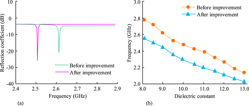
Figure 7. The variation linearity of simulated resonant frequency and dielectric constant of high-temperature sensor before and after improvement. (a) Simulation resonance frequency of high temperature sensor before and after improvement. (b) Linear change in dielectric constant of temperature sensor before and after improvement.

To verify the impedance matching performance and signal reflection stability of the improved sensor in different dielectric environments, a comparative analysis is conducted on the reflection coefficients of the high-temperature sensor before and after improvement under different dielectric constants. The dielectric constants are 9, 10, 11, and 12, respectively. The results are shown in Figure 8. In Figure 8a, before the sensor improvement, the reflection coefficients with dielectric constants of 9 and 10 reached their peak values when the resonant frequencies were 2.54 GHz and 2.50 GHz, respectively. When the resonant frequencies were 2.43 GHz and 2.28 GHz, the reflection coefficients with dielectric constants of 11 and 12 were −21.36 dB and −19.98 dB, respectively. In Figure 8b, after improving the sensor, the reflection coefficients with dielectric constants of 9 and 10 reached their peak values at 2.46 GHz and 2.35 GHz, respectively. When the resonant frequencies were 2.27 GHz and 2.17 GHz, the reflection coefficients with dielectric constants of 11 and 12 were −40.076 dB and −44.82 dB, respectively. The results show that the improved high-temperature sensor exhibits better impedance matching performance and signal reflection stability in different dielectric environments.

Figure 8

Figure 8. Reflection coefficients of high-temperature sensors before and after improvement under different dielectric constants. (a) Reflection coefficient of sensor improvement before improvement. (b) Reflection coefficient of sensor improvement after improvement.

The simulation results and test results of the improved sensor are compared at room temperature, and the reflection coefficient is analyzed at different temperatures, as displayed in Figure 9. Figure 9a shows the comparison between the simulated and tested reflection coefficients of the improved sensor at room temperature, with the sensor sample placed in the testing fixture during measurement. The results showed that when the resonant frequency was 2.34 GHz, the simulated reflection coefficient reached its peak at room temperature, which was −37.56 dB. When the resonant frequency was 2.32 GHz, the tested reflection coefficient reached its peak, at −37.62 dB. The minor frequency shift is primarily attributed to fabrication tolerances and subtle deviations in material properties between the ideal simulation model and the physically realized sensor. In Figure 9b, when the resonant frequencies were 2.43 GHz, 2.38 GHz, and 2.33 GHz, the reflection coefficients were −38.27 dB, −42.78 dB, and −40.15 dB, respectively. When the resonant frequencies were 2.28 GHz, 2.24 GHz, and 2.19 GHz, the reflection coefficients were −35.26 dB, −38.69 dB, and −36.13 dB, respectively. The results show that the improved sensor exhibits excellent performance in both room temperature and high-temperature environments.

Figure 9

Figure 9. Simulation results of improved sensors and analysis of reflection coefficient characteristics in high-temperature environments. (a) Comparison of simulation results and test results after sensor improvement. (b) Reflection coefficient results of improved sensors at different temperatures.

To verify the temperature stability and optimization effect of the resonant frequency of the sensor, the linear fitting curve of the resonant frequency before and after improving the temperature sensor at different temperatures is analyzed, and the frequency temperature coefficient is compared, as displayed in Figure 10. In Figure 10a, before the sensor improvement, when the temperature reached 1,000 °C, the resonant frequencies were 2.33 GHz and 2.35 GHz, respectively. After improving the sensor, the resonant frequencies of actual testing and data processing at 1,000 °C were 2.13 GHz and 2.14 GHz, respectively. In Figure 10b, before improving the sensor, when the temperature increased from 200 °C to 1,000 °C, the frequency temperature coefficient decreased from −12.48 ppm/°C to −14.23 ppm/°C. After improving the sensor, the frequency temperature coefficient increased from −5.25 ppm/°C to −3.76 ppm/°C. The results show that the improved sensor has less variation in resonant frequency at different temperatures, reduced sensitivity to temperature changes, and better frequency temperature stability.

Figure 10

Figure 10. Linear fitting curve of resonant frequency and frequency temperature coefficient before and after improvement of temperature sensor. (a) Linear fitting curve of resonant frequency before and after improvement of temperature sensor. (b) Comparison of frequency temperature coefficient before and after improvement of temperature sensor.

The quality factor, sensitivity, electromagnetic coupling efficiency, and deformation coefficient of the high-temperature sensor before and after improvement are compared at different temperatures to comprehensively evaluate the overall performance of the sensor in high-temperature environments, as displayed in Figure 11. In Figure 11a, at 1,000 °C, the quality factor and sensitivity of the sensor before improvement were 241 and 10.89 GHz, respectively, while the quality factor and sensitivity after improvement were 418 and 17.12 GHz, respectively. In Figure 11b, at 1,000 °C, the electromagnetic coupling efficiency and deformation coefficient of the sensor before improvement were 0.87 and 2.82 × 10⁻⁶ K⁻¹ Pa⁻¹, respectively, while the electromagnetic coupling efficiency and deformation coefficient after improvement were 418 and 17.12 × 10⁻⁶ K⁻¹ Pa⁻¹, respectively. The improved sensor has improved quality factor, sensitivity, electromagnetic coupling efficiency, and deformation coefficient at different temperatures.

Figure 11

Figure 11. Comparison results of comprehensive performance before and after temperature sensor improvement. (a) Quality factor and sensitivity of temperature sensors before and after improvement. (b) Electromagnetic coupling efficiency and deformation coefficient before and after temperature sensor improvement.

3.2 Analysis of high temperature test results for back-end circuit measurement system

To verify the performance of the back-end circuit measurement system in ultra-high temperature environments, the designed back-end circuit measurement system collects data from the improved temperature sensor and analyzes the error between the resonant frequency measured by the network analyzer and the measured data. The results are shown in Figure 12. In Figure 12a, when the resonant frequency was between 2.0 GH and 2.6 GHz, the collected voltage of the improved sensor was between 0.52 V and 2.27 V. In Figure 12b, when the resonant frequency was 2.32 GHz, the reflection coefficient tested by the network analyzer was −37.89 dB. When the resonant frequency was 2.30 GHz, the reflection coefficient tested by the proposed system was −37.72 dB. Its resonant frequency error was only 0.02 GHz. The results show that the back-end circuit measurement system can effectively collect data and has good consistency with the results tested by the network analyzer.

Figure 12

Figure 12. Comparative analysis of data acquisition between network analyzer and circuit measurement system. (a) Data acquisition results of improved temperature sensor. (b) Data acquisition results of network analyzer and circuit measurement system.

The circuit test results of the network analyzer and the designed system are compared at different temperatures. The error frequency and test error are analyzed, as displayed in Figure 13. In Figure 13a, at 200 °C, the resonant frequencies of the network analyzer and the proposed system were 2.39 GHz and 2.36 GHz, respectively. At 1,000 °C, their frequencies were 2.09 GHz and 2.10 GHz, respectively. In Figure 13b, at 200 °C, the frequency error and test error between the network analyzer and the proposed system were 0.021 GHz and 0.74%, respectively. At 600 °C, the frequency error and test error were 0.002 GHz and 0.08%, respectively. The measurement results of the proposed system at different temperatures have small errors compared to the results of the network analyzer, indicating that the system has excellent reliability in practical applications.

Figure 13

Figure 13. Error analysis between network analyzer and designed system at different temperatures. (a) Electromagnetic coupling efficiency and deformation coefficient before and after temperature sensor improvement. (b) Frequency error and test error between network analyzer and designed system.

4 Discussion and conclusion

A new sensor scheme based on CSRR structure optimization was proposed to address the performance deficiencies of passive wireless sensors in ultra-high temperature environments. A dedicated back-end circuit measurement system was developed to support the improved sensor. The simulation results showed that the quality factor of the improved sensor increased from 241 to 418 at different temperatures, the sensitivity increased from 10.89 to 17.12, the electromagnetic coupling efficiency increased from 0.87 to 1.23, and the deformation coefficient decreased from 2.82 to 1.56. The sensitivity to temperature changes was reduced, and the frequency temperature coefficient was optimized from −14.23 ppm/°C to −3.76 ppm/°C. The resonant frequency changed less, showing better temperature stability. The back-end circuit measurement system in ultra-high temperature environment showed good consistency with the test results of the network analyzer, with a resonance frequency error of only 0.02 GHz and a test error of less than 1%. While many existing studies have successfully demonstrated high sensitivity in liquid or microfluidic sensing at room temperature (Haq and Koziel, 2022; Han et al., 2024), their operational scope often does not extend to ultra-high temperature environments. In contrast, the sensor developed in this work is specifically designed and optimized for such extreme conditions. The proposed folded CSRR sensor exhibits a notably high quality factor of 418 and a significantly low-frequency temperature coefficient of −3.76 ppm/°C at 1,000 °C. These key metrics underscore a decisive advantage in thermal stability over previously reported designs. For instance, the high-Q microstrip sensor in (Zegadi et al., 2025), while excellent for high-resolution dielectric characterization at room temperature, lacks reported high-temperature performance data. Similarly, the optimized sensor in (Haq and Koziel, 2022) and the compact sensor in (Vaidya et al., 2025) focus primarily on sensitivity enhancement for specific applications but do not address the critical issue of frequency drift with temperature.

The results indicate that the improved passive wireless high-temperature sensor and its back-end circuit measurement system proposed in the study can effectively enhance the stability, sensitivity, and measurement accuracy in ultra-high temperature environments. The limitation of this study is that it does not take into account the long-term high-temperature aging effect of the sensor. In the future, material processes can be optimized and machine learning algorithms can be introduced to enhance the long-term stability and adaptability of sensors.

Data availability statement

The original contributions presented in the study are included in the article/supplementary material, further inquiries can be directed to the corresponding author.

Author contributions

DL: Software, Methodology, Data curation, Conceptualization, Writing – review and editing, Writing – original draft, Project administration, Supervision.

Funding

The authors declare that no financial support was received for the research and/or publication of this article.

Conflict of interest

The author declares that the research was conducted in the absence of any commercial or financial relationships that could be construed as a potential conflict of interest.

Generative AI statement

The authors declare that no Generative AI was used in the creation of this manuscript.

Any alternative text (alt text) provided alongside figures in this article has been generated by Frontiers with the support of artificial intelligence and reasonable efforts have been made to ensure accuracy, including review by the authors wherever possible. If you identify any issues, please contact us.

Publisher’s note

All claims expressed in this article are solely those of the authors and do not necessarily represent those of their affiliated organizations, or those of the publisher, the editors and the reviewers. Any product that may be evaluated in this article, or claim that may be made by its manufacturer, is not guaranteed or endorsed by the publisher.

References

Aprile, A., Folz, M., Gardino, D., Malcovati, P., and Bonizzoni, E. (2023). An area-efficient smart temperature sensor based on a fully current processing error-feedback noise-shaping SAR ADC in 180-nm CMOS. IEEE J. Solid-State Circuits 59 (3), 716–727. doi:10.1109/JSSC.2023.3342937

CrossRef Full Text | Google Scholar

Athar, S., Patel, G., Xu, Z., Qiu, Q., and She, Y. (2023). VisTac toward a unified multimodal sensing finger for robotic manipulation. IEEE Sensors J. 23 (20), 25440–25450. doi:10.1109/JSEN.2023.3310918

CrossRef Full Text | Google Scholar

Bandewad, G., Datta, K. P., Gawali, B. W., and Pawar, S. N. (2023). Review on discrimination of hazardous gases by smart sensing technology. Artif. Intell. Appl. 1 (2), 70–81. doi:10.47852/bonviewAIA3202434

CrossRef Full Text | Google Scholar

Buragohain, A., Das, G. S., Beria, Y., Kalita, P. P., and Mostako, A. T. T. (2023). Highly sensitive DS-CSRR based microwave sensor for permittivity measurement of liquids. Meas. Sci. Technol. 34 (12), 125134–125148. doi:10.1088/1361-6501/acf336

CrossRef Full Text | Google Scholar

Das, G. S., Buragohain, A., and Beria, Y. (2024). Microwave differential CSRR sensor for liquid permittivity measurement. J. Electron. Mater. 53 (7), 3541–3547. doi:10.1007/s11664-024-11060-6

CrossRef Full Text | Google Scholar

Dawn, N., Ghosh, S., Saha, A., Chatterjee, S., Ghosh, T., Guha, S., et al. (2024). A review on digital twins technology: a new frontier in agriculture. Artif. Intell. Appl. 2 (4), 250–262. doi:10.47852/bonviewAIA3202919

CrossRef Full Text | Google Scholar

Grosinger, J., and Michalowska-Forsyth, A. (2022). Space tags: ultra-low-power operation and radiation hardness for passive wireless sensor tags. IEEE Microw. Mag. 23 (3), 55–71. doi:10.1109/MMM.2021.3130686

CrossRef Full Text | Google Scholar

Gu, S., Sun, W., Li, M., Zhang, T., and Deng, M. (2022). Highly sensitive plasmonic refractive index sensor based on dual D-shaped photonic crystal fiber with aluminum nitride-silver films. Plasmonics 17 (3), 1129–1137. doi:10.1007/s11468-022-01609-8

CrossRef Full Text | Google Scholar

Han, C., Wang, Y., Li, Y., Chen, Y., Abbasi, N. A., Kuerner, T., et al. (2022). Terahertz wireless channels: a holistic survey on measurement, modeling, and analysis. IEEE Commun. Surv. and Tutorials 24 (3), 1670–1707. doi:10.1109/COMST.2022.3182539

CrossRef Full Text | Google Scholar

Han, X., Peng, P., Fu, C., Qiao, L., Ma, Z., Liu, K., et al. (2024). Highly integrated improved hexagonal CSRR-based fluid sensor for complex dielectric parameter detection. IEEE Sensors J. 24 (13), 20559–20570. doi:10.1109/JSEN.2024.3399454

CrossRef Full Text | Google Scholar

Haq, T., and Koziel, S. (2022). Inverse modeling and optimization of CSRR-based microwave sensors for industrial applications. IEEE Trans. Microw. Theory Tech. 70 (11), 4796–4804. doi:10.1109/TMTT.2022.3176886

CrossRef Full Text | Google Scholar

Jiang, S., Liu, G., Wang, M., Wu, Y., and Zhou, J. (2023). Design of high-sensitivity microfluidic sensor based on CSRR with interdigital structure. IEEE Sensors J. 23 (16), 17901–17909. doi:10.1109/JSEN.2023.3294243

CrossRef Full Text | Google Scholar

Kumar, K. S., and Madhan, M. G. (2025). Analysis of a CSRR-based S-Band microstrip patch structure for sensor and tunable antenna applications. Int. J. Appl. Electromagn. Mech. 77 (3), 202–214. doi:10.1177/13835416251318335

CrossRef Full Text | Google Scholar

Li, C., Zheng, S., Hui, X., and Zhang, X. (2024). Electromagnetic effective coupling and high spatial resolution theory in near-field cardiac sensing. IEEE Trans. Microw. Theory Tech. 72 (4), 2283–2297. doi:10.1109/TMTT.2023.3346680

CrossRef Full Text | Google Scholar

Ma, L., Lu, J., Gu, C., and Mao, J. (2022). A wideband dual-circularly polarized, simultaneous transmit and receive (STAR) antenna array for integrated sensing and communication in IoT. IEEE Internet Things J. 10 (7), 6367–6376. doi:10.1109/JIOT.2022.3225339

CrossRef Full Text | Google Scholar

Nagmani, A. K., and Behera, B. (2024). Design and performance analysis of a high-temperature sensor with a low-temperature coefficient of frequency. J. Electron. Mater. 53 (5), 2488–2497. doi:10.1007/s11664-024-10969-2

CrossRef Full Text | Google Scholar

Prakash, D., and Gupta, N. (2022). High-sensitivity grooved CSRR-based sensor for liquid chemical characterization. IEEE Sensors J. 22 (19), 18463–18470. doi:10.1109/JSEN.2022.3198837

CrossRef Full Text | Google Scholar

Rahim, M. K. A., Samsuri, N. A., Wijayanto, Y. N., and Yusuf Nur Wijayanto, (2023). Substrate comparison on multiband reflector performance for intelligent reflecting surfaces (IRSs). ELEKTRIKA-Journal Electr. Eng. 22 (2), 56–61. doi:10.11113/elektrika.v22n2.457

CrossRef Full Text | Google Scholar

Shinde, K. S., Shah, S. N., and Patel, P. N. (2024). Design and simulation of planar microwave sensor for food industry. J. Korean Phys. Soc. 85 (1), 35–46. doi:10.1007/s40042-024-01097-5

CrossRef Full Text | Google Scholar

Swarna, S., and Kolluru, V. R. (2024). Active channel selection by sensors using artificial neural networks. Int. J. Electr. Electron. Res. 12 (4), 1466–1473. doi:10.37391/IJEER.120441

CrossRef Full Text | Google Scholar

Teo, T. Y., Krbal, M., Mistrik, J., Prikryl, J., Lu, L., and Simpson, R. E. (2022). Comparison and analysis of phase change materials-based reconfigurable silicon photonic directional couplers. Opt. Mater. Express 12 (2), 606–621. doi:10.1364/OME.447289

CrossRef Full Text | Google Scholar

Vaidya, A., Tvsnd, K., Kalantari, A., and Sainkar, S. (2025). Compact CSRR based sensor for detection of impurities in liquid samples. Sens. Imaging 26 (1), 52–14. doi:10.1007/s11220-025-00583-9

CrossRef Full Text | Google Scholar

Xiao, H., Yan, S., Guo, C., and Chen, J. (2022). A dual-scale CSRRs-based sensor for dielectric characterization of solid materials. IEEE Sensors Lett. 6 (12), 1–4. doi:10.1109/LSENS.2022.3224445

CrossRef Full Text | Google Scholar

Yan, J., Cheng, Y., Zhang, L., Li, Z., Xu, T., Zhang, F., et al. (2023). Displacement field reconstruction technique for plate-like structures based on model superposition method. Meas. Control 56 (3-4), 654–667. doi:10.1177/00202940221095535

CrossRef Full Text | Google Scholar

Zegadi, R., Sayad, D., Mekki, S., Bouknia, M. L., Tighilt, Y., Alzuraiqi, E., et al. (2025). High Q-factor CSRR-loaded microstrip sensor for high-resolution complex permittivity characterization. Opt. Quantum Electron. 57 (6), 376–390. doi:10.1007/s11082-025-08284-z

CrossRef Full Text | Google Scholar