 Ryan W. Paerl1*
 Kenneth S. Johnson2
 Rory M. Welsh2 Alexandra Z. Worden2 Francisco P. Chavez2 and Jonathan P. Zehr1
- 1 Department of Ocean Sciences, University of California Santa Cruz, Santa Cruz, CA, USA
- 2 Monterey Bay Aquarium Research Institute, Moss Landing, CA, USA
Synechococcus is an abundant marine cyanobacterial genus composed of different populations that vary physiologically. Synechococcus narB gene sequences (encoding for nitrate reductase in cyanobacteria) obtained previously from isolates and the environment (e.g., North Pacific Gyre Station ALOHA, Hawaii or Monterey Bay, CA, USA) were used to develop quantitative PCR (qPCR) assays. These qPCR assays were used to quantify populations from specific narB phylogenetic clades across the California Current System (CCS), a region composed of dynamic zones between a coastal-upwelling zone and the oligotrophic Pacific Ocean. Targeted populations (narB subgroups) had different biogeographic patterns across the CCS, which appear to be driven by environmental conditions. Subgroups C_C1, D_C1, and D_C2 were abundant in coastal-upwelling to coastal-transition zone waters with relatively high to intermediate ammonium, nitrate, and chl. a concentrations. Subgroups A_C1 and F_C1 were most abundant in coastal-transition zone waters with intermediate nutrient concentrations. E_O1 and G_O1 were most abundant at different depths of oligotrophic open-ocean waters (either in the upper mixed layer or just below). E_O1, A_C1, and F_C1 distributions differed from other narB subgroups and likely possess unique ecologies enabling them to be most abundant in waters between coastal and open-ocean waters. Different CCS zones possessed distinct Synechococcus communities. Core California current water possessed low numbers of narB subgroups relative to counted Synechococcus cells, and coastal-transition waters contained high abundances of Synechococcus cells and total number of narB subgroups. The presented biogeographic data provides insight on the distributions and ecologies of Synechococcus present in an eastern boundary current system.
Introduction
The picocyanobacterial (unicellular cyanobacteria <2 μm in diameter) genus Synechococcus is considered to be cosmopolitan in the ocean, occurring at concentrations ranging from ∼102 to 106 cells ml−1 in open-ocean and coastal waters (Waterbury et al., 1979, 1986; Partensky et al., 1999). Multiple lineages of Synechococcus are present in the ocean (Herdman et al., 2001; Rocap et al., 2002; Dufresne et al., 2008) and isolates from these lineages vary physiologically in regards to their pigmentation, motility, responses to light, and ability to assimilate nitrogen (N) forms (Waterbury et al., 1985; Palenik, 2001; Moore et al., 2002; Fuller et al., 2003; Ahlgren and Rocap, 2006; Six et al., 2007).
Nitrate is one N form that can be assimilated by many, but not all, Synechococcus isolates (Moore et al., 2002; Fuller et al., 2003; Scanlan et al., 2009). Nitrate is important in the ocean because it fuels a significant amount of “new” production, particularly in upwelling influenced environments (Dugdale and Goering, 1967). The narB gene, which encodes for a cyanobacterial assimilatory nitrate reductase enzyme (Rubio et al., 1996), has been used to selectively study Synechococcus potentially capable of nitrate assimilation (Ahlgren and Rocap, 2006; Jenkins et al., 2006; Paerl et al., 2008). Some Synechococcus strains lack the narB gene (e.g., RS9917, Dufresne et al., 2008), therefore examining narB sequence diversity is complementary to the use of more common phylogenetic markers used for studying complete Synechococcus diversity (e.g., the 16S rRNA gene, 16S-23S ITS region, rpoC gene; Palenik, 1994; Rocap et al., 2002; Fuller et al., 2003). This approach of studying the narB gene can provide information on the diversity and gene expression of nitrate-assimilating Synechococcus populations.
The spatial distribution of different Synechococcus clades has not been studied across the transition zones of an upwelling-influenced, eastern-boundary current system such as the California Current System (CCS). Recently, abundances of 16S rRNA-defined Synechococcus clades have been tracked on a northwest Arabian Sea transect (Fuller et al., 2006) and on large-scale open-ocean transects (Zwirglmaier et al., 2007, 2008). In this study, we targeted populations (called narB subgroups) belonging to different narB clades that were initially found in either coastal or open-ocean habitats (Jenkins et al., 2006; Paerl et al., 2008). Subgroup abundances were tracked across distinct water masses of the CCS to further investigate their biogeography and how distributions are related to the dynamics of coastal systems. The CCS was an ideal system for examining Synechococcus biogeography because it possesses several chemically and biologically distinct regions (Chavez et al., 1991; Collins et al., 2003), all of which are anticipated to harbor Synechococcus populations (Collier and Palenik, 2003; Worden et al., 2004; Tai and Palenik, 2009). Multiple narB subgroup abundance profiles were obtained using newly developed narB quantitative PCR (qPCR) assays and applying them to depth profile samples from different regions of the CCS.
Materials and Methods
Sample Collection
Seawater samples were collected from depth using a SeaBird 12 PVC Niskin bottle conductivity–temperature–depth (CTD) rosette while onboard the R/V Western Flyer (October 1–10, 2007; cruise CN207). CTD profiles were conducted at six stations on CalCOFI line 67 (Lynn et al., 1982) and six cyclonic eddy stations (Figure 1). Core oceanographic CTD samplings (for nutrients, chl. a, etc.) were performed with greater frequency than nucleic acid filtrations. Light measurements were recorded directly from the CTD during rosette deployments.
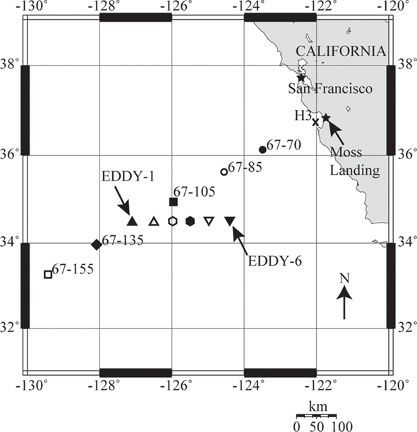
Figure 1. A map of nucleic acid sampling stations on cruise CN207, which follow CalCOFI line 67. The coastal-upwelling zone station H3 is marked by an X, coastal-transition zone stations 67–70 and 67–85 are marked with solid and hollow circles, core California Current (CC) station 67–105 is marked by a solid square, CC transition station 67–135 is marked with a solid diamond and oligotrophic open-ocean station 67–155 is marked with a hollow square. Upward and downward triangles and hexagons mark individual cyclonic eddy stations. The map was generated using OMC (http://www.aquarius.ifm-geomar.de/).
Core Oceanographic Measurements
Seawater samples collected for nitrate, nitrite, and phosphate analysis were frozen and stored at −20°C onboard immediately after collection from the CTD rosette. Nutrient concentrations in these samples were analyzed in the laboratory by automated chemical analysis using standard colorimetric methods (Sakamoto et al., 1990). Ammonium was determined onboard as described by Plant et al. (2009). Chl. a and phaeopigments were determined fluorometrically using a Turner Designs Model 10-005 R fluorometer that was calibrated with a commercial chl. a standard (Sigma, St. Louis, MO, USA). Samples for determination of pigments were filtered onto 25 mm GF/F glass fiber filters (Whatman, Piscataway, NJ, USA) and extracted in 90% (v/v) acetone in a −20°C freezer for between 24 and 30 h (Venrick and Hayward, 1984). Other than the modification of the extraction procedure, the method used is the conventional fluorometric procedure of Holm-Hansen et al. (1965) and Lorenzen (1966).
DNA Collection and Extraction
Environmental DNA was obtained using the collection and extraction methods described by Paerl et al. (2008). Briefly, seawater was collected from the CTD rosette and emptied into polycarbonate bottles. Collected seawater was filtered using a peristaltic pump with in-line 25 mm, 10 and 0.22 μm pore size filters. Filters were stored onboard in liquid nitrogen immediately after filtration. DNA was extracted from cells collected upon filters using a modified DNeasy Plant Kit (Qiagen, Valencia, CA, USA) procedure as detailed by Paerl et al. (2008).
Phylogenetic Analysis and narB qPCR Primer Probe Design
Prior to designing narB qPCR primer probe sets, narB gene sequences from Synechococcus cultures and uncultivated environmental populations were compiled into a database and aligned using the ARB software package (Ludwig et al., 2004) as described by Paerl et al. (2008). Sequences were exported from ARB and phylogenetic trees were constructed using the MEGA3 program (Kumar et al., 2004). Seven different qPCR primer-probe sets (with dual-labeled oligonucleotide probes) were designed using Primer Express 3.0 software (Applied Biosystems, Carlsbad, CA, USA) and sequences from different Synechococcus narB gene clades (Table 1; Figure 2). Target narB sequences for qPCR assays were considered to be narB sequences with less than three mismatches to the qPCR assay oligonucleotides (three total mismatches across primers and probe; listed in Table A1 in Appendix). Three mismatches were determined to be the appropriate cutoff based on previous qPCR amplification efficiency tests that showed three total mismatches between template and qPCR oligonucleotides results in approximately an order of magnitude underestimation of the template concentration (Short and Zehr, 2005). Two mismatches between template and qPCR oligonucleotides have no effect on the quantification of target concentrations (K. Turk and J. Zehr, unpublished). Names for each narB qPCR assay corresponds to a targeted narB clade (Paerl et al., 2008; Figure 2). The C (coastal) or O (open-ocean) designation in the assay name indicates whether targeted sequences for the assay include those originally obtained from coastal or open-ocean sites.
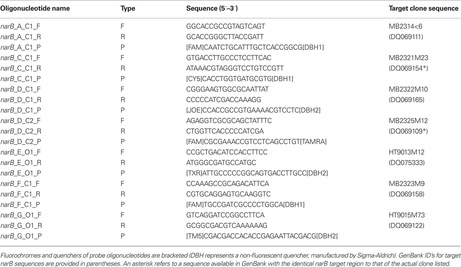
Table 1. Primers and probe components for each of the developed narB qPCR assays.
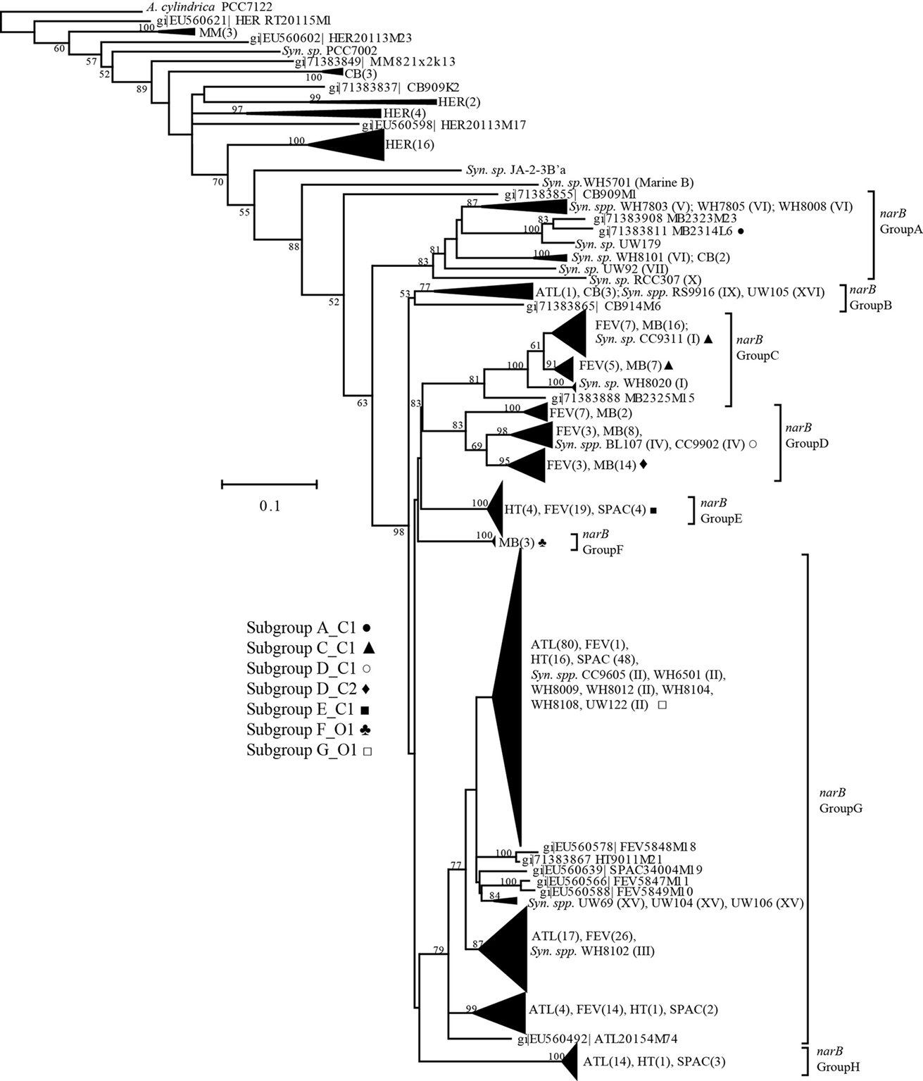
Figure 2. A phylogenetic tree of aligned narB sequences from Synechococcus isolates and environmental samples. The tree was constructed using a neighbor-joining, Jukes-Cantor corrected method in MEGA3 (Kumar et al., 2004). Bootstrap values were obtained from the generation of 1000 replicate trees initialized with a random seed. Bootstrap values <50 are not shown. Next to collapsed branches are abbreviated sequence names (unique to the sampling site, e.g., ATL, N. Atlantic) and the number of these sequences in branch. narB cluster names are from Paerl et al. (2008) and are next to bracketed regions of the tree. Synechococcus isolates that have been classified into a major Synechococcus clade (e.g., based on the 16S rRNA gene, ITS, rpoC) are marked with their respective clade numeral. GenBank accession numbers for sequences within narB clusters have been omitted for brevity, but are listed in Paerl et al. (2008). GenBank ID’s for the narB sequences of Synechococcus isolates are included in Table A2 in Appendix. narB qPCR assay names are in bold text next to identifier symbols, and corresponding symbols are next to targeted clusters of the narB tree.
narB qPCR Assays
Quantitative PCR reactions were performed using the plasmid standard curve approach described by Short and Zehr (2005) with modifications. Plasmid standards were synthesized by ligating a specific narB PCR product into a pGEM vector (Promega; Madison, WI, USA). The vector plus insert was used to transform JM109 (E. coli) competent cells following the protocol of the manufacturer (Promega). JM109 cells possessing a pGEM vector plus insert were screened from LB agar plates containing X-GAL, carbenicillin, and IPTG. White colonies were selected from plates and grown overnight in liquid SOC media plus carbenicillin at 37°C with shaking at 320 rpm. Purified plasmid was recovered from transformed cells using the QIAprep Spin Miniprep Kit (Qiagen).
In vitro primer probe cross-reactivity tests were conducted in duplicate using a dilution series (100–108 or 109 copies) of target and non-target plasmid standards (restriction digested pGEM vectors containing a known narB clone insert). Non-target plasmid standards used in these tests were the target standards for other narB qPCR assays and had a minimum of eight total mismatches to primer and probes of the tested narB qPCR assay.
The abundances of narB gene copies in environmental DNA samples were determined by analyzing CT values of triplicate reactions (with environmental DNA) with the linear regression of CT values from duplicate plasmid standard reactions. For each qPCR run, threshold and baseline values were automatically calculated using the 7500 software package (Applied Biosystems), treating each measurement as a unique run. narB qPCR assays were designed using different fluorophores (for future use in multiplex reactions). The narB subgroup E_O1 probe utilized a Texas Red fluorophore requiring ROX (a background dye in the Applied Biosystems MasterMix) detection to be disabled and the baseline to be set manually at the mid-exponential region of the amplification signal.
The qPCR quantification limits were calculated for environmental samples based on the sample volumes and amplification limits of plasmid standards. The theoretical limit of quantification for narB qPCR assays was 125 copies l−1, based on the detection of a single gene copy from 2 l of filtered seawater, a DNA elution volume of 50 μl, 1:10 dilution of the DNA extract to avoid inhibition and a 2-μl addition of diluted extracted to the qPCR reaction. The actual limit of quantification was higher because <10 plasmid standard copies was not consistently detected per qPCR reaction, making the actual limit of quantification 1250 gene copies l−1 (1.25 copies ml−1) of seawater. Template detected below this quantification limit (<10 copies per reaction) in ≥2 reactions was considered detected but not quantifiable (DNQ). Template was considered undetected when ≥2 reactions showed no amplification signal. Individual qPCR assay amplification efficiencies were calculated using the following formula,  where m is the slope of the linear regression between CT values of the linear plasmid standard curve (Table 2).
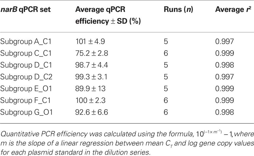
Table 2. Average reaction efficiency for each narB qPCR assay.
In this study we assumed abundance estimates from the narB qPCR assays (narB gene copies ml−1) equate to cells ml−1 since all complete cyanobacterial genomes sequenced to-date possess single copies of the narB gene. This assumption could lead to overestimation of narB subgroups if targeted narB genes are also on multiple genomes, plasmids, and/or viral genomes within a single Synechococcus cell.
Flow Cytometry Based Synechococcus Counts
Flow cytometry (FCM) samples were collected and fixed with glutaraldehyde (0.25%, final concentration) in parallel with collected nucleic acid samples at stations 67–70, 67–85, 67–105, 67–155, EDDY-2, EDDY-3, and EDDY-4. Additional FCM samples were collected from C1 (MBARI mooring), 67–65, 67–95, and 67–115 (data not shown). Samples were analyzed on a Becton Dickinson (Franklin Lakes, NJ, USA) InFlux flow cytometer (formerly Cytopeia) equipped with a 488-nm laser (200 mW output). Forward angle light scatter (FALS), right angle light scatter (RALS), orange fluorescence from phycoerythrin (527 ± 27 nm), and red fluorescence from chl. a (692 ± 40 nm) were measured after 488 nm laser excitation. Yellow Green fluorescent beads (0.75 μm diameter) were added to samples prior to analysis for later signal normalization. Samples were delivered at ∼25 μl min−1 for 2 min prior to data collection, to ensure equilibration of the sample line. The sample was then stopped, weighed, restarted along with data acquisition, and weighed again at the end of the run to precisely determine the volume run. Data acquisition was triggered on FALS. Data were analyzed using WinList (Verity Software House; Topsham, ME, USA). Synechococcus were identified and enumerated on the basis of light scatter and fluorescence signals as described previously (Olson et al., 1990), with orange-fluorescence being a defining characteristic of phycoerythrin containing Synechococcus. Small “green” Synechococcus-like cells were not used for comparisons with qPCR data in order to avoid including counts that potentially represented picoeukaryotes.
Correlation and Multi-Dimensional Scaling Analysis
All CN207 data was log (1 + x) transformed before generation of correlation matrices and multi-dimensional scaling (MDS) plots. Spearman correlation matrices and MDS plots were generated in XLSTAT (Addinsoft; New York, NY, USA). Spearman matrices were used because the majority of measured variables failed multiple normality tests. An absolute MDS model was run in XLSTAT using a Spearman proximity similarity matrix, and the MDS model utilized a random initial configuration, a 2–4 dimension evaluation and 500 cumulative iterations.
Results
qPCR Cross-Reactivity Tests
Quantitative PCR specificity tests with non-target standards (listed in Table 1) yielded either no amplification signal or an amplification signal at a CT number (the cycle in which amplification of template crosses the exponential amplification threshold) larger than the CT number obtained from amplification of a target standard (Figure 3). Non-target standards yielded equivalent CT numbers to target standards when the concentrations of non-target plasmid standards were ∼1000 times greater than target standards. For example, the narB subgroup D_C1 assay exhibited non-specific amplification (false positive) from 104 copies of the subgroup F_C1 target plasmid (a mean CT value of ∼37, equivalent to ∼10 narB gene copies of subgroup D_C1; Figure 3).
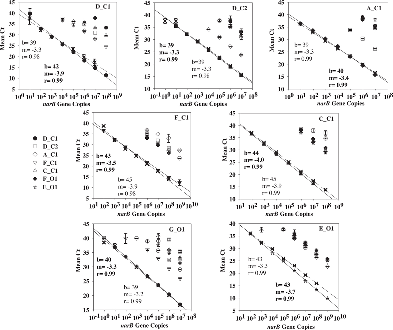
Figure 3. Cross-reactivity tests for each narB qPCR assay using target and non-target plasmid standards (listed in Table 1). Target standard data are the solid symbols (X’s are secondary qPCR runs) and include a linear fit line (solid line for solid symbols, dashed line for X’s). Linear fit data in bold corresponds to the solid linear fit line.
Hydrographic Conditions
Contrasting chemical and biological conditions were evident among sampling stations (Figure 4), all of which are generally consistent with prior oceanographic observations made along line 67 (Collins et al., 2003). Coastal-upwelling zone surface waters (station H3) had high concentrations of nitrate (∼10 μmol l−1) and chl. a (>2 μg l−1). Coastal-transition zone profiles (stations 67–70 and 67–85) possessed slightly lower chl. a concentrations (>0.50 μg l−1) in the upper surface layer and a more dramatic nitracline (where nitrate surpassed 1 μmol l−1) at ∼0–30 m. At stations 67–70 and 67–85 entrainment of higher salinity water from below was evident to a depth of 100 m (Figure 4), indicating these waters were likely part of a filament of previously upwelled seawater transported offshore. Open-ocean conditions were present at stations 67–105 to 67–155, as they possessed deep chl. a maxima and nitraclines (∼60–90 m) with very low chl. a (<0.20 μg l−1) and nitrate (<0.20 μmol l−1) concentrations in the upper ∼40 m (Figure 4). However, conditions varied among these open-ocean stations. Station 67–105 was located within the core of the California Current (CC), as seen by the low salinity (<33) feature in the upper 100 m, 300 to 600 km offshore (Figure 4). Station 67–135 was in a transition from CC conditions to N. Pacific gyre-like conditions, based on the increase in salinity in the upper 100 m and deepening of the chl. maximum (∼100 m) relative to station 67–105. Salinity in the upper 100 m of station 67–155 increased further and conditions are closest to those of oligotrophic N. Pacific water gyre water (Figure 4).
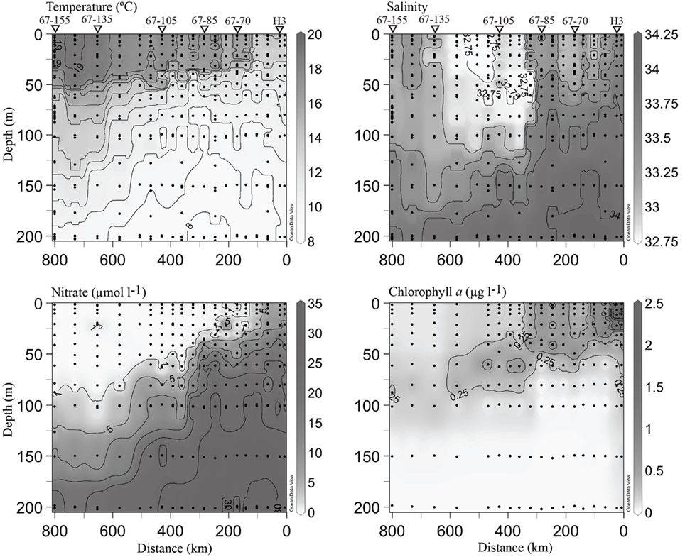
Figure 4. Hydrographic conditions along the line 67 transect from Moss Landing, CA (0 km) to station 67–155 (∼800 km from shore). Black circles indicate locations of discrete measurements collected via the CTD rosette. Contour lines are drawn on intervals of 1, 0.25, 5, and 0.25 for individual temperature, salinity, nitrate and chl. a plots. Values are included for maximal and minimal contours. A 1-μmol l−1 nitrate contour line has been drawn to emphasize the beginning of the nitracline. Triangles and station names at the top of the plot indicate where DNA samples were collected. All plots were generated using Ocean Data View (http://odv.awi.de).
Core cyclonic eddy waters (EDDY-3, EDDY-4) possessed physical and chemical conditions comparable to those observed in the coastal-transition zone (stations 67–85, 67–70), including a shallow nitracline (∼50 m), high chl. a (>0.5 μg l−1) in the upper 40 m, and high salinity water in the upper 60 m (Figure 5). Outside of the eddy core (stations EDDY-1, EDDY-2, EDDY-5, and EDDY-6), the halocline and nitracline were deeper (∼125 m) resembling conditions at open-ocean sites along the CN207 transect (e.g., 67–135 and 67–155; Figures 4 and 5).
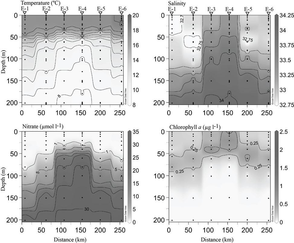
Figure 5. Hydrographic conditions across a cyclonic eddy. Black circles indicate locations of discrete sampling. Contouring was generated as in Figure 4. Triangles at the top of the plot indicate stations where DNA samples were collected. Eddy station names have been abbreviated with the letter E for clarity.
narB Subgroup Distributions
Abundances of subgroups E_O1 and G_O1 were highest at open-ocean station 67–155 (76 and 285 copies ml−1 respectively, Figure 7). These subgroups were also detected in at station 67–85 and core eddy profiles, but in concentrations below quantifiable limits (Figures 7 and 8). Abundance maxima of the open-ocean subgroups (called O subgroups herein) occurred at different depths, with subgroup G_O1 being most prominent in the upper mixed layer (upper 40 m) and subgroup E_O1 most abundant just below subgroup G_O1 (∼60 m; Figure 7). This distribution disparity was also evident in periphery cyclonic eddy profiles (Figure 8).
narB subgroups originally found in coastal habitats (those ending in C1 or C2, called C subgroups herein) were most abundant in euphotic waters of coastal-transition (67–70 and 67–85), coastal (H3) and core eddy stations (Figures 7 and 8). Maximalabundances of these subgroups (aside from subgroup D_C1) were an order of magnitude higher than the maxima of O subgroups, and occurred >100 km from the coast (stations 67–70, 67–85, EDDY-3, and EDDY-4; Figures 7 and 8). In some cases, C subgroup abundances decreased by three orders of magnitude (e.g., subgroup F_C1, 4.7 × 10³ copies ml−1 to DNQ) from the coastal-transition zone to more oligotrophic CC waters (station 67–105; Figure 7). C subgroups were detected in open-ocean profiles (67–105 and beyond) but in low abundances (e.g., <24 subgroup C_C1 narB gene copies ml−1 were present at stations 67–105, 67–135, and 67–155; Figure 7).
Subgroup D_C2 reached the highest abundance of all the narB subgroups examined (>8.0 × 10³ copies ml−1) and was quantifiable at all stations between depths of 0–50 m (Figures 7 and 8). Subgroup D_C1 and C_C1 were less abundant than D_C2, but exhibited similar distribution patterns (Figures 7 and 8). C_C1 reached maximum abundance at ∼50 m of station 67–70 (2.5 × 10³ copies ml−1). D_C1 abundances were notably low at all stations relative to other C subgroups (Figures 7 and 8). Cross reactivity of the subgroup D_C1 probe set with F_C1 and D_C2 targets may have contributed a false positive for this subgroup at stations 67–85, 67–70, and EDDY-2 where F_C1 and D_C2 target abundances were close to 104 copies ml−1 (Figures 7 and 8). Subgroup A_C1 and F_C1 distributions contrasted with those of D_C1, D_C2, and C_C1, as they were most abundant at <25 m of transitional stations 67–70 and 67–85. Of the two, F_C1 reached a higher maximum abundance (7.0 × 10³ versus 2.3 × 10³ copies ml−1) in profile samples and was present over a broader range of stations and depths (Figures 7 and 8).
MDS Analysis
Measured variables (triangles) clustered differently in the MDS coordinate space (Figure 9). The spacing of variables in the MDS plot is a visual representation of the Spearman correlation matrix (Table 3). Subgroup C_C1 clustered relatively close to chl a, ammonium, and nitrate, but was distant from temperature. Subgroups D_C1, D_C2 clustered close to subgroup C_C1, and one another while also being close to ammonium, nitrate, and chl. a. Subgroups A_C1 and F_C1 clustered with each other and with PAR (photosynthetically active radiation), but were more distant from ammonium, nitrate and chl. a than subgroups D_C1 and D_C2. Subgroups E_O1 and G_O1 both clustered distantly from inorganic nutrients and C subgroups, but differed in their spacing along dimension two in which depth was strongly positive (Figure 9A). Total narB subgroup abundances clustered with environmental variables in a similar fashion to D_C2 and F_C1, the two most abundant narB subgroups (Figure 9A).
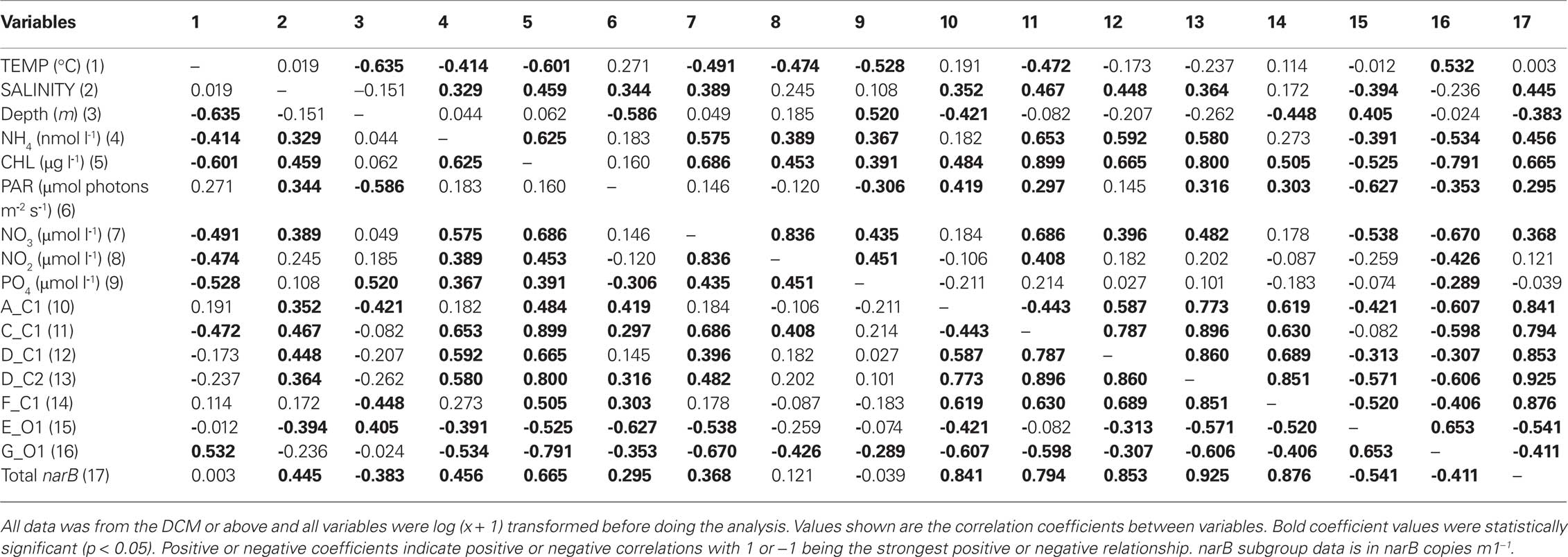
Table 3. A Spearman correlation matrix of subgroup abundances and environmental variables.
The relationship between nitrate, a nutrient found to significantly correlate with subgroup abundances (Table 3), was examined further with a second bubble MDS plot (Figure 9B), and in scatter plots (Figure 10). The bubble MDS plot (based on abundance data only) indicated narB subgroups were separated in the projection space as seen in the initial MDS plot (spacing is randomly initialized, so their coordinate placement differs), and that three different correlation types were evident: strongly positive, weakly positive, and strongly negative. Subgroups A_C1 and F_C1 had weak correlation coefficients of ∼0.18 that were not significant (p > 0.05; Figure 9B; Table 3). Scatter plots of subgroup abundance versus nitrate vary congruently with the MDS bubble plot (Figure 9B), and data points were either closer to being positively linear, negatively linear, or non-monotonic (Figure 10). Comparable results were seen when ammonium values were examined instead of nitrate, and when phosphate was compared, correlations and fits on the scatter plots (r2 values) were weaker (data not shown), which was expected based on the initial MDS plot and correlation matrix (Figure 9A; Table 3).
FCM Synechococcus Counts
Synechococcus cell abundances ranged from ∼103 to 105 cells ml−1 in the upper mixed layer of line 67 and cyclonic eddy station profiles. At all stations, maximal Synechococcus cell abundances occurred in the upper water column and decreased below 40–60 m (Figure 6). The highest abundance of Synechococcus cells in a single sample was observed at 0 m of station 67–85 (8.6 × 10⁴ cells ml−1). Synechococcus cell abundances in the upper water column were higher in coastal-upwelling and coastal-transition zones than in open-ocean waters (e.g., at 0 m of station 67–155, ∼2 × 10³ cells ml−1; Figure 6). Similarly, Synechococcus abundances were higher (5.2 × 10⁴ cells ml−1) in the surface waters of core cyclonic eddy stations EDDY-3 and -4 (0–20 m, Figure 6), and fewer in surface waters of outer eddy station EDDY-2 (0 m, 8.2 × 10³ cells ml−1; data not shown).
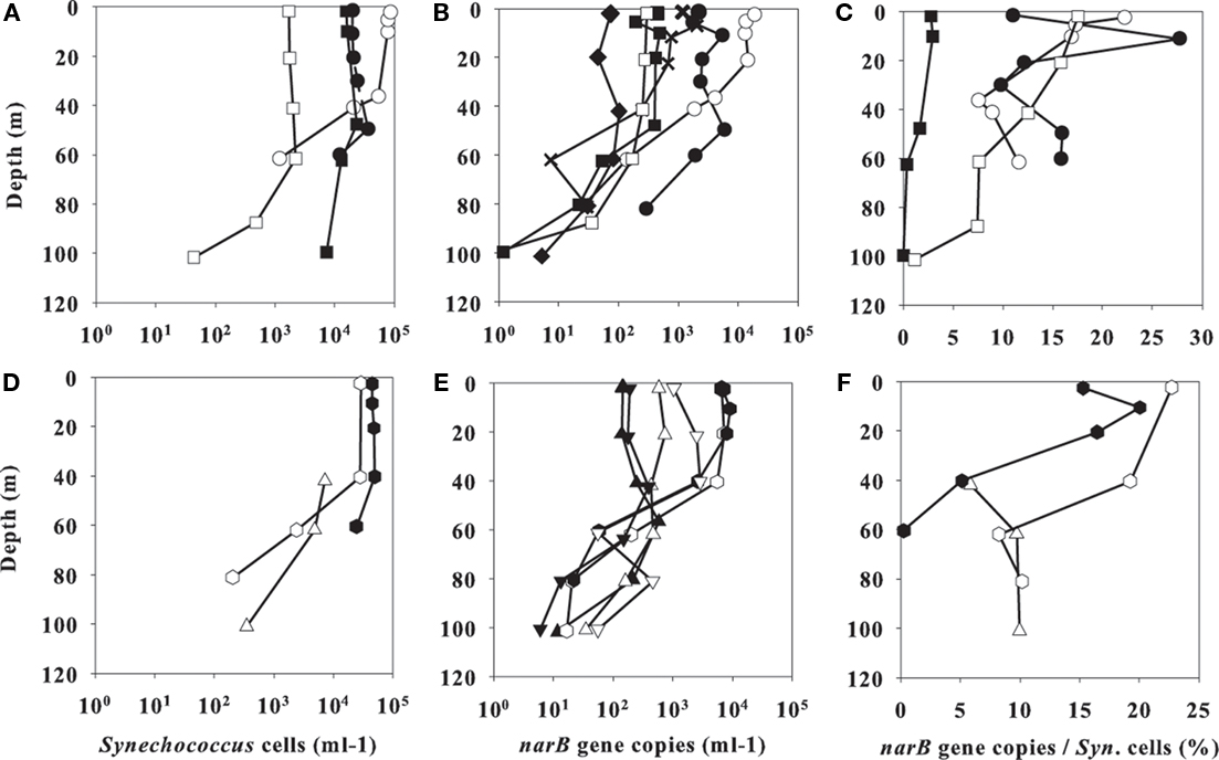
Figure 6. Profile data from line 67 stations (A–C) or cyclonic eddy stations (D–F). FCM-based Synechococcus cell counts are in (A,D), total abundances of examined narB subgroups are in (B,E), and percent total narB subgroup abundances/Synechococcus cell counts from the same samples are in (C,F). Station symbols are consistent with those in Figure 1. Note the linear scale on the x-axis of (C,F).
Discussion
Different Distributions of O and C Subgroups
Contour plots of abundance and environmental data indicate that narB subgroups inhabited different water masses along the CCS transect (Figures 7 and 8). Previous studies showed that Synechococcus narB sequence diversity differed between coastal and open-ocean sampling sites (Jenkins et al., 2006; Paerl et al., 2008). This is also seen in the data of this study as narB C and O subgroups co-occurred in samples but their abundances were not comparable (Figures 7 and 8). However, the qPCR data provides further biogeographic data that shows populations (subgroups) belonging to narB sequence clades initially related to coastal or open-ocean waters actually exhibit different distributions across multiple CCS water masses. C subgroups initially found within and just offshore of MB (Jenkins et al., 2006) inhabit the coastal-upwelling zone, but also the coastal-transition zone that extended roughly 200 km offshore (Figures 3 and 7). The O subgroups previously found in open-ocean sequence libraries, were most abundant at different depths of the euphotic zone in oligotrophic CCS waters (Figures 7 and 8). The qPCR data indicates that Synechococcus populations in the CCS do not simply increase with closer proximity to the coast, or with chl. a, which is more the case with eukaryotic phytoplankton, e.g., diatoms (Chavez et al., 1991). Instead, there appears to be a progression of different Synechococcus populations across the transition from coastal to open-ocean. Temporal change in narB subgroup distributions across the CCS or at a given site within the CCS was not examined in this study. Hydrographic conditions across the CCS change seasonally (Lynn et al., 1982; Lynn and Simpson, 1987) and as a result distributions of narB subgroups, particularly C subgroups, are also expected to seasonally vary.
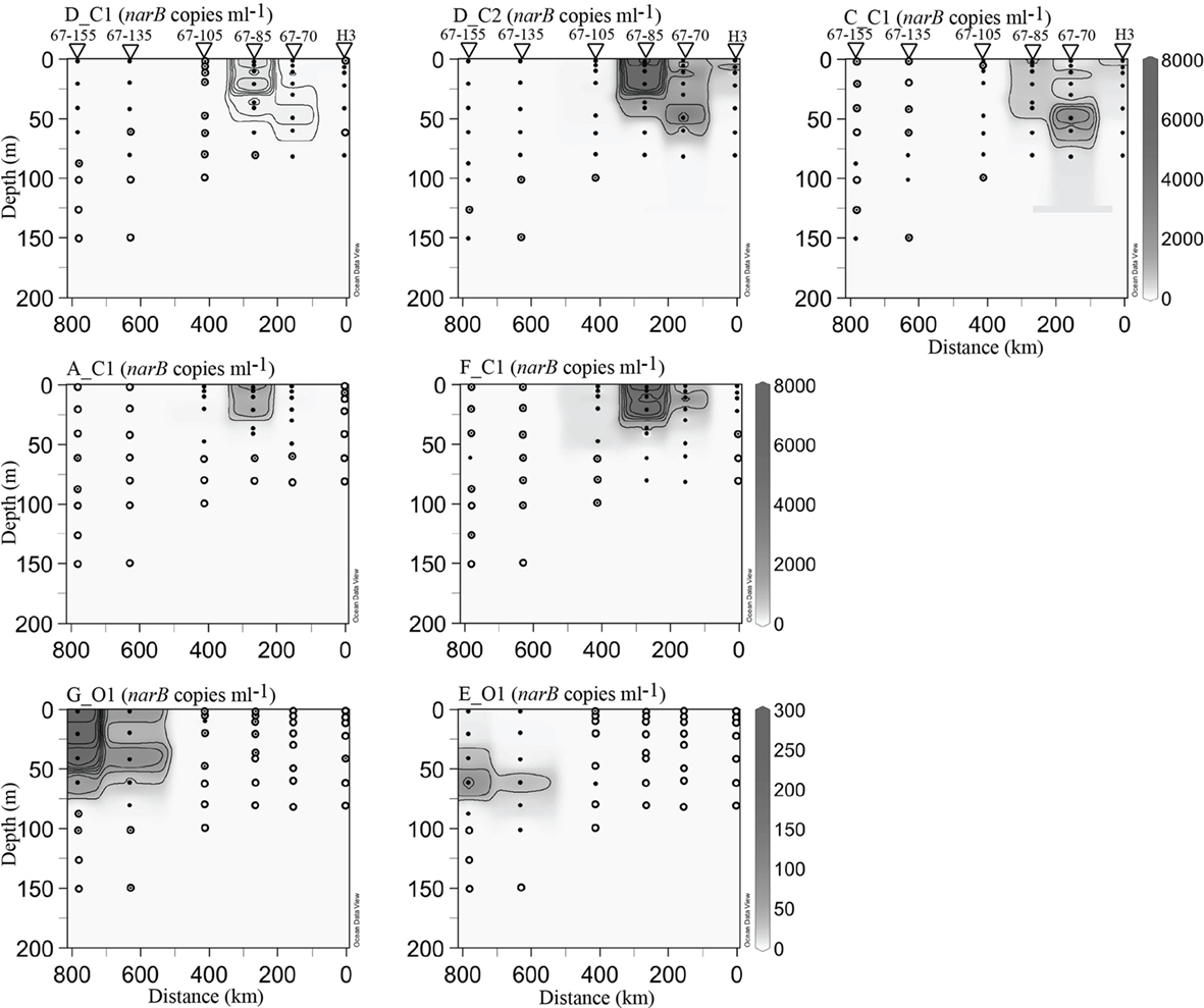
Figure 7. narB subgroup abundances along profiles from station H3 to station 67–155 (see Figure 1). The abundance scale (z-axis) is in gene copies ml−1. Black circles mark samples containing quantifiable amounts of narB subgroups, concentric circles mark locations where subgroups were detected but not quantifiable and hollow circles mark locations where narB subgroups were undetected. Note the different abundance scales used for coastal (C) and open-ocean (O) subgroups. Contour intervals vary based on the narB subgroup plot: E_O1 and, G_O1 25 narB copies ml−1; D_C1, 50 narB copies ml−1; A_C1 and C_C1, 500 narB copies ml−1; D_C2 and F_C1, narB 1000 copies ml−1.
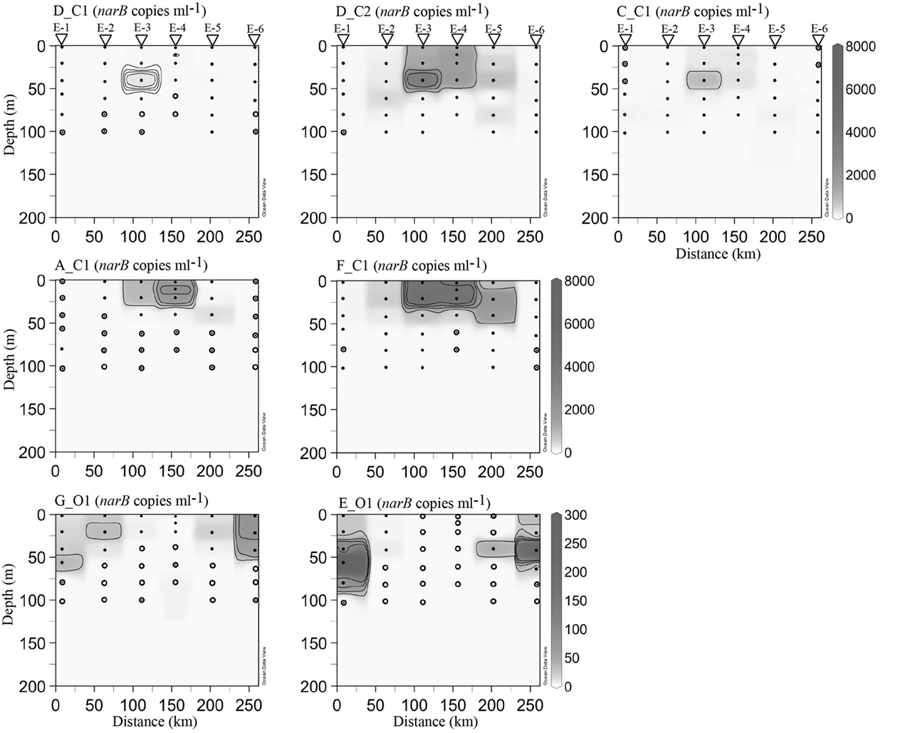
Figure 8. narB subgroup abundances in cyclonic eddy station profiles. Contouring and sample marks were done as described for Figure 7. Eddy station names have been abbreviated with the letter E for clarity.
Two large-scale flows within the central CCS, the CC and an inshore surface pole-ward flow, vary seasonally (Lynn and Simpson, 1987) and likely impact distributions of narB subgroups across the CCS. Also, the occurrence of strong seasonal upwelling (in the spring) is expected to affect narB subgroup distributions. Abundances of all narB subgroups were notably low in the core CC (around station 67–105) suggesting that they are unable to thrive in this water mass (Figure 7). During the late fall (as sampled in this study) and winter, the core CC narrows and migrates offshore. This potentially broadens the coastal-transition zone where multiple C subgroups appear able to thrive (Figure 7). Additionally during the fall, surface seawater temperatures are at their warmest and mixing is reduced (upwelling is at a minimum), which favors increased cyanobacterial growth. Therefore, C narB subgroups are anticipated to be most abundant and occupy the largest area of the CCS (the coastal-upwelling and coastal-transition zones) during the fall. In the late fall and winter, a pole-ward surface flow occurs off the CA coast (Lynn and Simpson, 1987). This flow is expected to lead to increased mixing in the coastal-upwelling zone (along with winter storms) and narrow the coastal-transition zone where subgroups A_C1 and F_C1 are present (and presumably adapted to conditions of the transitional waters, see Figure 7). Greatest narrowing of the coastal-transition zone is expected to occur during the spring, when the CC broadens and migrates toward the coast, and maximal upwelling occurs in the coastal-upwelling zone. Lastly, non-seasonal variation in C subgroup abundances is also expected in the region between core CC water and the coastal-upwelling zone due to the frequent occurrence of eddies (as seen in this study) and meanderings of the CC (Lynn and Simpson, 1987).
Distinct Distributions of narB Subgroups Suggest Differences in their Ecologies
The distinct distributions of narB subgroups across the CCS presumably result from selection by different environmental conditions. Subgroups D_C1, D_C2, and C_C1 are able to persist in coastal-upwelling and coastal-transition zone waters containing relatively high to intermediate nutrients, cooler temperatures, higher salinity, and elevated chl. a (Figures 4, 7, and 9). Based on narB gene sequences, these subgroups cluster with isolates belonging to clades I and IV (Figure 2), which are common clades in temperate, coastal waters (Zwirglmaier et al., 2008; Tai and Palenik, 2009). These subgroups varied in their abundances at depth within the coastal-transition zone, suggesting light or some other factor(s) related to depth may differentially affect their numbers. Also C_C1, D_C1, and D_C2 vary in their abundances within the coastal-upwelling and coastal-transition zone, suggesting they differ in their growth or mortality. For example, abundances of D_C1 were low relative to C_C1 and D_C2. It is unknown whether D_C1 reaches higher abundances at other times of the year or are more abundant in waters closer to the coast than station H3 (Figure 7).
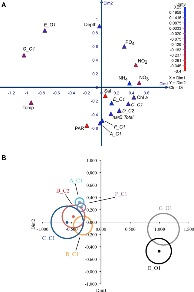
Figure 9. Multi-dimensional scaling plots of environmental variables and narB subgroup abundances from CN207 samples. Spearman similarity matrices were used to construct the MDS plots. All data used is from the DCM and above, and were log (x + 1) transformed before any analysis. narB subgroup abundance variables are italicized while environmental variables are not. (A) 3D plot of environmental and abundance variables, with the third dimension being represented by color (Kruskal’s stress = 0.08). (B) 2D MDS bubble plot of narB subgroup abundances (dots) and their respective correlation coefficients in relation to nitrate (bubbles; Kruskal’s stress = 0.04). A Spearman similarity matrix that contained only subgroup abundance data [same as in 9(A)] was used to construct the plot. Bubbles are scaled so that their width equates to the Spearman correlation coefficient value between the abundance of the respective subgroup and nitrate. All correlation coefficient values were significant (p < 0.05) except for subgroups A_C1 and F_C1 (small bubbles). Colored bubbles represent positive coefficients and grayscale bubbles are for negative values. The width of the largest bubble (C_C1) equates to 0.68, while the smallest bubbles equate to ∼0.18.
Subgroups A_C1 and F_C1 were most abundant in the upper water column (<25 m) of the coastal-transition zone where levels of nutrients, chl. a and/or covarying factors were lower than in coastal waters. Previous studies have associated increases of Synechococcus or a specific clade to increased nutrient concentrations in natural systems (Lindell and Post, 1995; DuRand et al., 2001; Fuller et al., 2006), but none have specifically linked increases in Synechococcus abundance with “intermediate” nutrient conditions, which appears to be the case with subgroups F_C1 and A_C1 (Figure 10). Subgroups F_C1 and A_C1 are not represented by an isolate based on current narB phylogeny (Figure 2). Potentially they fit as “opportunists,” as has been suggested for Synechococcus clades V, VI, and VII (Fuller et al., 2006; Zwirglmaier et al., 2008; Dufresne et al., 2008), but specifically these “opportunists” appear to reach highest numbers in waters with intermediate levels of nitrate, ammonium and/or covarying factors (Figures 4, 7, and 9). Subgroup F_C1 in particular may be ecologically important in the coastal-transition zone since its abundance was comparable to or greater than abundances of subgroups D_C2 and C_C1 in this zone (Figure 7).
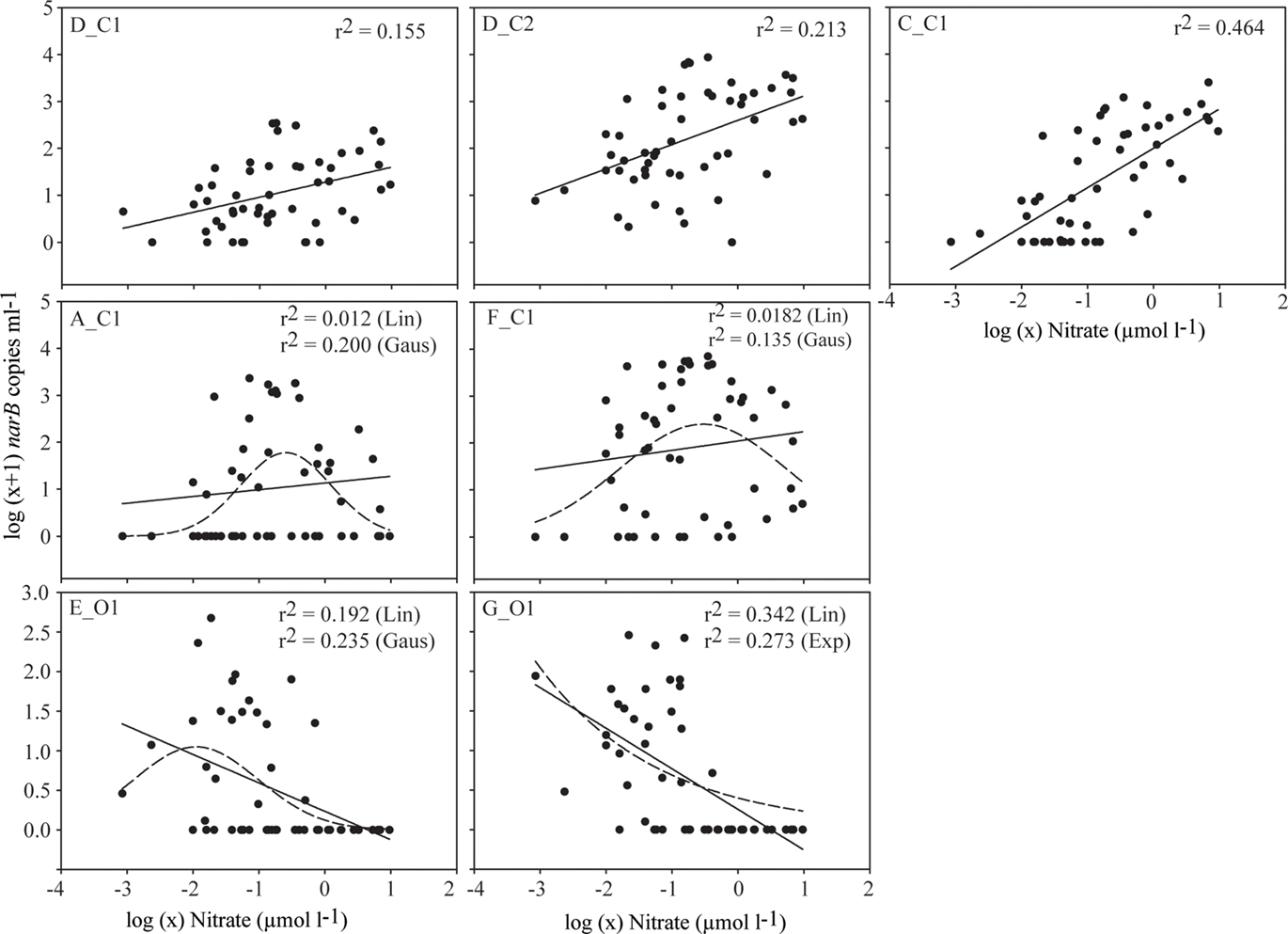
Figure 10. Scatter plots of narB subgroup abundance (log (x + 1) transformed) versus nitrate concentrations [log (x) transformed] in CN207 samples at the DCM or above. Fits are plotted to emphasize pattern differences in the data associated with each subgroup (e.g., changes in r2 and direction of the slope). Non-linear fits are plotted as dashed lines. The r2 values are provided for all plotted fits.
O subgroups persisted at different depths of N. Pacific gyre-like waters with low nutrients and low phytoplankton biomass (chl. a). Subgroup G_O1 was most abundant in the upper mixed layer (Figures 7 and 8) as has been previously described for clade II Synechococcus (Toledo and Palenik, 2003; Zwirglmaier et al., 2008). G_O1 also clusters with clade II isolates based on narB gene phylogeny (Figure 2). A factor or factors related to depth enables subgroup E_O1 to be most abundant in relatively deep euphotic waters just below the upper mixed layer (Figures 7 and 8). This distribution is consistent with additional observations from the subtropical N. Pacific station ALOHA and an oligotrophic open-ocean station (26.5°N, 110.3°W) off the coast of Baja, Mexico (R.W. Paerl, R.A. Foster and J.P. Zehr, unpublished). The E_O1 distribution pattern contrasts with that of G_O1 (Figures 7 and 8), but also the typical near-uniform abundances of Synechococcus cells in the upper mixed layer of open-ocean depth profiles (Waterbury et al., 1986; Partensky et al., 1999).
It is anticipated that the E_O1 subgroup is composed of Synechococcus, not Prochlorococcus. To our knowledge, no Synechococcus strain, clade, or ecotype is currently recognized to predominate below the upper mixed layer of oligotrophic open-ocean waters. Some Prochlorococcus populations appear to possess the narB gene (Martiny et al., 2009) and some also persist at depth (West and Scanlan, 1999; Johnson et al., 2006), but the majority of Prochlorococcus narB genes identified thus far resemble high light (HL) Prochlorococcus in their percentage G + C content (∼30–40%; Martiny et al., 2009), and a few linked to low light (LL) Prochlorococcus strains have percentage G + C ∼40%. All of these Prochlorococcus associated narB genes have lower percentage G + C than narB clade Group E sequences (∼60%; Paerl et al., 2008). We have constructed several amino acid phylogenetic trees based on clustalW aligned portions of NarB sequences from environmental samples (Jenkins et al., 2006; Paerl et al., 2008), Synechococcus genomes, and putative HL Prochlorococcus NarB sequences identified by Martiny et al. (2009). In these trees Prochlorococcus NarB sequences are clearly divergent from Synechococcus isolate sequences as reported by Martiny et al. (2009), but also narB clade E amino acid sequences (data not shown).
Other environmental conditions that were not measured could also influence the distribution of narB subgroups. Metal concentrations were not measured, yet metals such as Fe can be introduced into the euphotic zone via vertical mixing in waters off the coast of CA (Martin and Gordon, 1988) and the effects of metal species (e.g., Cu2+ and Ni) could be stimulatory or deleterious to Synechococcus growth (Brand et al., 1986; Dupont et al., 2008; Stuart et al., 2009). Zooplankton grazing and viral lysis were not measured at CN207 stations, but should be examined in future studies as they could also alter Synechococcus abundances in the CCS.
The Potential Role for NR Encoded by the narB Gene
The Synechococcus NR encoded by the narB gene could be used in nitrate assimilation or in the reduction of intracellular energy generated by photosynthesis (e.g., ferredoxin, ATP). Natural Synechococcus populations (off the FL coast) assimilated  in on-deck incubation experiments (Wawrik et al., 2009), so presumably narB is being expressed, translated, and the NR enzyme is reducing nitrate for the synthesis of macromolecules like DNA. However, it is still feasible that nitrate reduction could be used as mechanism to deplete intracellular energy from the photosystem, especially under conditions of high irradiance and high nitrate, as has been observed in coastal diatoms (Lomas and Glibert, 1999). In the open-ocean, it is unlikely that nitrate reduction is being used as a mechanism for dissipating energy from the photosystem, largely because concentrations of nitrate are very low and the complete assimilation of nitrate to glutamine would also be an effective sink of reductant and ATP while helping to alleviate N-based growth limitation. narB genes are present in the euphotic, oligotrophic open-ocean (Jenkins et al., 2006; Paerl et al., 2008; Martiny et al., 2009), and it is anticipated that the nitrate reductase encoded by these narB genes are used in the assimilation of nitrate, which may periodically become available via ammonia oxidation, eddies, or vertical mixing (McGillicuddy et al., 2007; Yool et al., 2007; Johnson et al., 2010). It does appear that the highest genetic potential for nitrate reduction by narB subgroups is in coastal-transition and coastal-upwelling zones of the CCS containing relatively intermediate to high concentrations of nitrate (Figure 6). Total narB subgroup abundance also clustered close to ammonium (and somewhat with nitrite) in the MDS analysis (Figure 8), which emphasizes that there is also a greater potential for these Synechococcus to assimilate N forms other than nitrate as well (Figure 8).
Comparisons of narB Subgroup Abundance and FCM-Based Synechococcus Counts
Total narB copies to FCM cell abundances as a percentage (narB copies/FCM counts × 100%) on average across comparable samples was ∼11% (data in Figure 6), which suggests that Synechococcus not targeted by our qPCR assays were present in our samples. This is not unexpected since the qPCR assays target a portion of the total Synechococcus diversity (Figure 2). However, this percentage value is actually difficult to interpret because for one, we are assuming that one narB copy equates to one cell, which may not be the case (as mentioned in narB qPCR Assays), and two, Synechococcus abundances determined by qPCR do not equate to FCM cell counts (qPCR estimates were found to be ∼40% of FCM estimates based on narB qPCR analysis of sorted Synechococcus CC9311 cells; data not shown). Relative changes in this percentage appear more useful and indicate Synechococcus community composition differs between CCS habitats. Specifically, in core CC waters (station 67–105) the percentage of total narB copies to FCM counts was low relative to the average from other stations (∼3 versus 13% in the upper 10 m; Figure 6). The southerly flowing CC core (seen as the fresher, cooler water around station 67–105, Figure 4) likely contained populations endemic to more northern waters (e.g., Alaskan gyre). Recent FCM-based cell counts from the CC to N. Pacific Gyre-like water (67–105 to 67–155) also suggest that picoplankton community composition in this region is unique relative to that of coastal and coastal-transition waters (T. Cambell and A. Z. Worden, unpublished).
Total narB subgroup abundances and FCM-based Synechococcus counts were highest in the coastal-transition zone (stations 67–70, 67–85; Figure 6). Previous studies have noted maximal Synechococcus abundances in transitional CCS waters (Collier and Palenik, 2003; Sherr et al., 2005), although the reasons for this maximum, and its size and frequency, remain unknown. Potentially this Synechococcus maximum occurs in the coastal-transition zone because of lowered concentrations of nutrients and metals in this zone, which enables multiple Synechococcus populations to better compete against larger phytoplankton (e.g., diatoms). Such conditions feasibly exist when coastal water is transported offshore via filaments, meanders, and/or eddies (Bernstein et al., 1977; Brink and Cowles, 1991) and the macronutrient and metal concentrations within this seawater are reduced by large phytoplankton or complexation with organic matter.
Conclusion
The results of this study indicate that Synechococcus subpopulations are distributed differently across the CCS, an upwelling-influenced, eastern boundary current system. Some of the narB subgroup distributions did not follow a clear open-ocean, coastal-ocean dichotomy. The “transitional” waters of the CCS appear to contain distinct Synechococcus populations relative to adjacent waters. The predominance of E_O1 below the upper mixed layer of open-ocean waters and A_C1 and F_C1 in the coastal-transition zone suggests that these narB subgroups possess unique ecologies relative to other narB subgroups and Synechococcus clades found primarily in the coastal or open-ocean.
There is a large diversity of Synechococcus in the ocean (including populations not yet isolated), but the different phenotypes attributed to this large diversity and the ecological benefits of these phenotypes are still being identified and described. The biogeographic data presented here contributes valuable observations related to the ecology of picocyanobacteria in the oceans. Such data will be useful for validating recent models that examine the relationship among species distributions, diversity, and ecology (e.g., the Darwin model; Follows et al., 2007; Goebel et al., 2010). Additionally, the presented distribution data allows future studies to more effectively target several interesting Synechococcus subgroups in the natural environment.
Conflict of Interest Statement
The authors declare that the research was conducted in the absence of any commercial or financial relationships that could be construed as a potential conflict of interest.
Acknowledgments
We thank the officers and crew of the R/V Western Flyer (2007) for field assistance. Many thanks for laboratory and field assistance to: Z. Wisotsky, S. Sakamoto, Z. Kolber, A. Engman, and M. Blum. Thanks are extended to A. Yannarell and P. Raimondi for statistical discussions, R. Foster and anonymous reviewers for feedback on the manuscript. This research was supported by the NSF Center for Microbial Oceanography: Research and Education (C-MORE; EF-0424599), and Gordon and Betty Moore Foundation Marine Microbiology Investigatorand MEGAMER grants (Jonathan P. Zehr). Additional support came from the David and Lucile Packard Foundation (Kenneth S. Johnson, Rory M. Welsh, Alexandra Z. Worden, Francisco P. Chavez).
References
Ahlgren, N. A., and Rocap, G. (2006). Culture isolation and culture-independent clone libraries reveal new marine Synechococcus ecotypes with distinctive light and N physiologies. Appl. Environ. Microbiol. 72, 7193–7204.
Bernstein, R. L., Breaker, L., and Whritner, R. (1977). California current eddy formation: ship, air, and satellite results. Science 195, 353–359.
Brand, L. E., Sunda, S. G., and Guillard, R. R. L. (1986). Reduction of marine phytoplankton reproduction rates by copper and cadmium. J. Exp. Mar. Biol. Ecol. 96, 225–250.
Brink, K. H., and Cowles, T. J. (1991). The coastal transition zone program. J. Geophys. Res. 96, 14637–14647.
Chavez, F. P., Barber, R. T., Kosoro, P. M., Huyer, A., Ramp, S. R., Stanton, T. P., and Mediola de, B. R. (1991). Horizontal transport and the distribution of nutrients in the coastal transition zone off Northern California: effects on primary production, phytoplankton biomass and species composition. J. Geophys. Res. 96, 14833–14848.
Collier, J. L., and Palenik, B. (2003). Phycoerythrin-containing picoplankton in the Southern California bight. Deep Sea Res. Part II Top. Stud. Oceanogr. 50, 2405–2422.
Collins, C. A., Pennington, J. T., Castro, C. G., Rago, T. A., and Chavez, F. P. (2003). The California current system off Monterey, California: physical and biological coupling. Deep Sea Res. Part II Top. Stud. Oceanogr. 50, 2389–2404.
Dufresne, A., Ostrowski, M., Scanlan, D. J., Garczarek, L., Mazard, S., Palenik, B. P., Paulsen, I. T., de Marsac, N. T., Wincker, P., Dossat, C., Ferriera, S., Johnson, J., Post, A. F., Hess, W. R., and Partensky, F. (2008). Unraveling the genomic mosaic of a ubiquitous genus of marine cyanobacteria. Genome Biol. 9, R90.
Dugdale, R. C., and Goering, J. J. (1967). Uptake of new and regenerated forms of nitrogen in primary productivity. Limnol. Oceanogr. 12, 196–206.
Dupont, C. L., Barbeau, K., and Palenik, B. (2008). Ni uptake and limitation in marine Synechococcus strains. Appl. Environ. Microbiol. 74, 23–31.
DuRand, M. D., Olson, R. J., and Chisholm, S. W. (2001). Phytoplankton population dynamics at the Bermuda Atlantic timeseries station in the Sargasso Sea. Deep Sea Res. Part II Top. Stud. Oceanogr. 48, 1983–2003.
Follows, M. J., Dutkiewicz, S., Grant, S., and Chisholm, S. W. (2007). Emergent biogeography of microbial communities in a model ocean. Science 315, 1843–1846.
Fuller, N. J., Marie, D., Partensky, F., Vaulot, D., Post, A. F., and Scanlan, D. J. (2003). Clade-specific 16S ribosomal DNA oligonucleotides reveal the predominance of a single marine Synechococcus clade throughout a stratified water column in the Red Sea. Appl. Environ. Microbiol. 69, 2430–2443.
Fuller, N. J., Tarran, G. A., Yallop, M., Orcutt, K. M., and Scanlan, D. J. (2006). Molecular analysis of picocyanobacterial community structure along an Arabian Sea transect reveals distinct spatial separation of lineages. Limnol. Oceanogr. 51, 2515–2526.
Goebel, N., Edwards, C. A., Zehr, J. P., and Follows, M. J. (2010). An emergent community ecosystem model applied to the California Current System. J. Mar. Syst. 83, 221–241.
Herdman, M., Castenholz, R. W., Iteman, I., Waterbury, J. B., and Rippka, R. (2001). “The cyanobacteria: subsection 1 (Formerly Chroococcales Wettstein 1924, emend. Rippka, Deruelles, Waterbury, Herdman and Stanier 1979),” in Bergey’s Manual of Systematic Bacteriology, eds D. R. Boone and R. W. Castenholz (New York: Springer), 493–514.
Holm-Hansen, O., Lorenzen, C. J., Holmes, R. W., and Strickland, J. D. (1965). Fluorometric determination of chlorophyll. J. Cons. Perm. Int. Explor. Mer. 30, 3–15.
Jenkins, B. D., Zehr, J. P., Gibson, A., and Campbell, L. (2006). Cyanobacterial assimilatory nitrate reductase gene diversity in coastal and oligotrophic marine environments. Environ. Microbiol. 8, 2083–2095.
Johnson, K. S., Riser, C. R., and Karl, D. M. (2010). Nitrate supply from deep to near-surface waters of the North Pacific subtropical gyre. Nature 465, 1062–1065.
Johnson, Z. I., Zinser, E. R., Coe, A., McNulty, N. P., Woodward, E. M. S., and Chisholm, S. W. (2006). Niche partitioning among Prochlorococcus ecotypes along ocean-scale environmental gradients. Science 311, 1737–1740.
Kumar, S., Tamura, K., and Nei, M. (2004). MEGA3: integrated software for molecular evolutionary genetics analysis and sequence alignment. Brief. Bioinform. 5, 150–163.
Lindell, D., and Post, A. F. (1995). Ultraphytoplankton succession is triggered by deep winter mixing in the Gulf of Aqaba (Eilat), Red Sea. Limnol. Oceanogr. 40, 1130–1141.
Lomas, M. W., and Glibert, P. M. (1999). Temperature regulation of nitrate uptake: a novel hypothesis about nitrate uptake and reduction in cool-water diatoms. Limnol. Oceanogr. 44, 556–572.
Lorenzen, C. J. (1966). A method for the continuous measurement of in vivo chlorophyll concentration. Deep Sea Res. 13, 223–227.
Ludwig, W., Strunk, O., Westram, R., Richter, L., Meier, H., Yadhukumar, Buchner, A., Lai, T., Steppi, S., Jobb, G., Förster, W., Brettske, I., Gerber, S., Ginhart, A. W., Gross, O., Grumann, S., Hermann, S., Jost, R., König, A., Liss, T., Lüssmann, R., May, M., Nonhoff, B., Reichel, B., Strehlow, R., Stamatakis, A., Stuckmann, N., Vilbig, A., Lenke, M., Ludwig, T., Bode, A., and Schleifer, K. H. (2004). ARB: a software environment for sequence data. Nucleic Acids Res. 32, 1363–1371.
Lynn, R. J., Bliss, K. A., and Eber, L. E. (1982). Vertical and horizontal distributions of seasonal mean temperature, salinity, sigma-t, stability, dynamic height, oxygen, and oxygen saturation in the California Current, 1950–1978. California Cooperative Oceanic Fisheries Investigations, Atlas, 30, 513.
Lynn, R. J., and Simpson, J. J. (1987). The California current system: the seasonal variability of its physical characteristics. J. Geophys. Res. 92, 12947–12966.
Martin, J. H., and Gordon, R. M. (1988). Northeast Pacific iron distributions in relation to phytoplankton productivity. Deep Sea Res. 35, 177–196.
Martiny, A. C., Kathuria, S., and Berube, P. M. (2009). Widespread metabolic potential for nitrite and nitrate assimilation among Prochlorococcus ecotypes. Proc. Natl. Acad. Sci. U.S.A. 106, 10787–10792.
McGillicuddy, D.J. Jr., Anderson, L. A., Bates, N. R., Bibby, T., Buesseler, K. O., Carlson, C. C., Davis, C. S., Ewart, C., Falkowski, P. G., Goldthwait, S. A., Hansell, D. A., Jenkins, W. J., Johnson, R., Kosnyrev, V. K., Ledwell, J. R., Li, Q. P., Siegel, D. A., and Steinberg, D. K. (2007). Eddy/wind interactions stimulate extraordinary midocean plankton blooms. Science 316, 1021–1026.
Moore, L. R., Post, A. F., Rocap, G., and Chisholm, S. W. (2002). Utilization of different nitrogen sources by the marine cyanobacteria Prochlorococcus and Synechococcus. Limnol. Oceanogr. 47, 989–996.
Olson, R. J., Zettler, E. R., Armbrust, E. V., and Chisholm, S. W. (1990). Pigment, size and distribution of Synechococcus in the North Atlantic and Pacific oceans. Limnol. Oceanogr. 35, 45–58.
Paerl, R. W., Foster, R. A., Jenkins, B. D., Montoya, J. P., and Zehr, J. P. (2008). Phylogenetic diversity of cyanobacterial narB genes from various marine habitats. Environ. Microbiol. 10, 3377–3387.
Palenik, B. (1994). Cyanobacterial community structure as seen from RNA polymerase gene sequence analysis. Appl. Environ. Microbiol. 60, 3212–3219.
Palenik, B. (2001). Chromatic adaptation in marine Synechococcus strains. Appl. Environ. Microbiol. 67, 991–994.
Partensky, F., Blanchot, J., and Vaulot, D. (1999). Differential distribution and ecology of Prochlorococcus and Synechococcus in oceanic waters: a review. Bull. Inst. Oceanogr. Monaco Numero Spec. 19, 457–475.
Plant, J. N., Johnson, K. S., Needoba, J. A., and Coletti, L. J. (2009). NH4-Digiscan: an in situ and laboratory ammonium analyzer for estuarine, coastal and shelf waters. Limnol. Oceanogr. Methods 7, 144–156.
Rocap, G., Distel, D. L., Waterbury, J. B., and Chisholm, S. W. (2002). Resolution of Prochlorococcus and Synechococcus ecotypes by using 16S-23S ribosomal DNA internal transcribed spacer sequences. Appl. Environ. Microbiol. 68, 1180–1191.
Rubio, L. M., Herrero, A., and Flores, E. (1996). A cyanobacterial narB gene encodes a ferredoxin-dependent nitrate reductase. Plant Mol. Biol. 30, 845–850.
Sakamoto, C. M., Friederich, G. E., and Codispoti, L. A. (1990). MBARI Procedures for Automated Nutrient Analyses Using a ModifiedAlpkem Series 300 Rapid Flow Analyzer. Monterey Bay Aquarium Research Institute, Technical Report 90-2, 84.
Scanlan, D. J., Ostrowski, M., Mazard, S., Dufresne, A., Garczarek, L., Hess, W. R., Post, A. F., Hagemann, M., Paulsen, I., and Partensky, F. (2009). Ecological genomics of marine Picocyanobacteria. Microbiol. Mol. Biol. Rev. 73, 249–299.
Sherr, E. B., Sherr, B. F., and Wheeler, P. A. (2005). Distribution of coccoid cyanobacteria and small eukaryotic phytoplankton in the upwelling ecosystem off the Oregon coast during 2001 and 2002. Deep Sea Res. Part II Top. Stud. Oceanogr. 52, 317–330.
Short, S. M., and Zehr, J. P. (2005). “Quantitative analysis of nifH genes and transcripts from aquatic environments,” in Methods in Enzymology, ed. J. Leadbetter (Amsterdam: Elsevier), 380–394.
Six, C., Thomas, J.-C., Garczarek, L., Ostrowski, M., Dufresne, A., Blot, N., Scanlan, D. J., and Partensky, F. (2007). Diversity and evolution of phycobilisomes in marine Synechococcus spp.: a comparative genomics study. Genome Biol. 8, R259.
Stuart, R. K., Dupont, C. L., Johnson, D. A., Paulsen, I. T., and Palenik, B. (2009). Coastal strains of marine Synechococcus species exhibit increased tolerance to copper shock and a distinctive transcriptional response relative to those of open-ocean strains. Appl. Environ. Microbiol. 75, 5047–5057.
Tai, V., and Palenik, B. (2009). Temporal variation of Synechococcus clades at a coastal Pacific Ocean monitoring site. ISME J 3, 903–915.
Toledo, G., and Palenik, B. (2003). A Synechococcus serotype is found preferentially in surface marine waters. Limnol. Oceanogr. 48, 1744–1755.
Venrick, E. L., and Hayward, T. L. (1984). Determining chlorophyll on the 1984 CalCOFI surveys. California Cooperative Oceanic Fish Investigations Report, 25, 74–79.
Waterbury, J. B., Watson, S. W., Guillard, R. R. L., and Brand, L. E. (1979). Widespread occurrence of a unicellular, marine, planktonic cyanobacterium. Nature 277, 293–294.
Waterbury, J. B., Watson, S. W., Valois, F. W., and Franks, D. G. (1986). “Biological and ecological characterization of the marine unicellular cyanobacterium Synechococcus,” in Photoynthetic Picoplankton, ed. W. K. W. Li (Ottawa: Department of Fisheries and Oceans), 71–120.
Waterbury, J. B., Willey, J. M., Franks, D. G., Valois, F. W., and Watson, S. W. (1985). A cyanobacterium capable of swimming motility. Science 230, 74.
Wawrik, B., Callaghan, A. V., and Bronk, D. A. (2009). Use of inorganic and organic nitrogen by Synechococcus spp. and diatoms on the west Florida shelf as measured using stable isotope probing. Appl. Environ. Microbiol. 75, 6662–6670.
West, N. J., and Scanlan, D. J. (1999). Niche-partitioning of Prochlorococcus populations in a stratified water column in the eastern North Atlantic ocean. Appl. Environ. Microbiol. 65, 2585–2591.
Worden, A. Z., Nolan, J. K., and Palenik, B. (2004). Assessing the dynamics and ecology of marine picophytoplankton: the importance of the eukaryotic component. Limnol. Oceanogr. 49, 168–179.
Yool, A., Martin, A. P., Fernandez, C., and Clark, D. R. (2007). The significance of nitrification for oceanic new production. Nature 447, 999–1002.
Zwirglmaier, K., Heywood, J. L., Chamberlain, K., Woodward, E. M. S., Zubkov, M. V., and Scanlan, D. J. (2007). Basin-scale distribution patterns of picocyanobacterial lineages in the Atlantic ocean. Environ. Microbiol. 9, 1278–1290.
Zwirglmaier, K., Jardillier, L., Ostrowski, M., Mazard, S., Garczarek, L., Vaulot, D., Not, F., Massana, R., Ulloa, O., and Scanlan, D. J. (2008). Global phylogeography of marine Synechococcus and Prochlorococcus reveals a distinct partitioning of lineages among oceanic biomes. Environ. Microbiol. 10, 147–161.
Keywords: Synechococcus, picocyanobacteria, biogeography, CCS, eastern-Pacific, qPCR, narB
Citation: Paerl RW, Johnson KS, Welsh RM, Worden AZ, Chavez FP and Zehr JP (2011) Differential distributions of Synechococcus subgroups across the California current system. Front. Microbio. 2:59. doi: 10.3389/fmicb.2011.00059
Received: 12 January 2011;
Paper pending published: 10 February 2011;
Accepted: 15 March 2011;
Published online: 04 April 2011.
Edited by:
Ian Hewson, Cornell University, USAReviewed by:
Jack A. Gilbert, Argonne National Laboratory, USATom Bibby, University of Southampton, UK
Copyright: © 2011 Paerl, Johnson, Welsh, Worden, Chavez and Zehr. This is an open-access article subject to a non-exclusive license between the authors and Frontiers Media SA, which permits use, distribution and reproduction in other forums, provided the original authors and source are credited and other Frontiers conditions are complied with.
*Correspondence: Ryan W. Paerl, Department of Ocean Sciences, University of California Santa Cruz, 1156 High Street EMS D402, Santa Cruz, CA 95064, USA. e-mail:cnBhZXJsQHVjc2MuZWR1