 Yingjie Mao
 Xiaoqian Li2
 Guicheng Zhang
 Jun Sun
- 1College of Marine Science and Technology, China University of Geosciences (Wuhan), Wuhan, China
- 2Research Centre for Indian Ocean Ecosystem, Tianjin University of Science and Technology, Tianjin, China
To examine the influence of mesoscale eddy on the natural phytoplankton community and its sinking rate changes, a comprehensive investigation cruise was carried out in the western South China Sea in autumn 2016. A total of 108 phytoplankton species were found, which belong to 54 phytoplankton genera; most of them were dominated by Dinophyta (54 genera), followed by Bacillariophyta (50 genera), Cyanophyta (3 genera), and Chrysophyta (1 genus). Bacillariophyta and Dinophyta were the main phytoplankton communities in the investigated sea area. The sinking rate of phytoplankton ranged from 0.12 to 3.17 m day–1, determined by the SETCOL method. The highest phytoplankton sinking rate was found in the 200-m water layer, followed by the DCM layer. No significant correlation was found between phytoplankton sinking rates and most of the environmental parameters during this cruise. At a similar time, we have carried out the estimation of carbon flux in the investigated sea area by using the sinking rate of phytoplankton, which showed that the carbon flux ranged from 2.41 × 10⁻⁶ to 0.006 mg C m–2 day–1; in addition, the maximum was at the 200-m layer. Phytoplankton community and sinking rate were significantly affected by the mesoscale eddy processes. The cold eddy could affect the community distribution of diatom and dinoflagellate, and the upwelling mainly affects the community of dinoflagellate. Both of them could contribute to a higher sedimentation rate of phytoplankton in the surface and DCM layers. Warm eddy could reduce the abundance of phytoplankton in the surface layer; simultaneously, the sinking rate of phytoplankton in the shallow water layer above 100 m is also reduced. These results can fill in the knowledge gap of mesoscale eddy processes in the study of phytoplankton community change and sinking rate; furthermore, it can provide insights into phytoplankton carbon and its implementation in further carbon sink.
Introduction
The largest ecosystem on earth is the marine ecosystem. The sea surface occupies nearly 71% of the earth’s surface, and seawater accounts for about 97.5% of the earth’s water (Peng, 2000). As a component and regulator in marine ecosystem, phytoplankton play an important role in the global carbon cycle (Sun, 2011). Phytoplankton can trap approximately 3 to 5 billion tons of carbon per year, which accounts for 40 to 50% of the world’s total primary productivity (Raymont, 2014). Although marine phytoplankton are tiny individuals and only account for 1% of the total global plant life, they fix as much net carbon dioxide as land plants, and perform nearly half of photosynthetic carbon fixation and half of the oxygen production (Hutchins and Boyd, 2016). In terms of spatial and temporal distribution, phytoplankton are more widely distributed and can respond more rapidly to environmental changes and, thus, are important to the global carbon cycle (Behrenfeld, 2014; Behrenfeld et al., 2017).
The South China Sea (SCS) is one of the largest semi-enclosed marginal sea, located in the tropical and subtropical regions of Southern Asia (Su, 2004; Guan and Yuan, 2006). The SCS, which is located in the East Asian monsoon region, has its own circulation structure, in which the circulation brought by the monsoon can affect the upper waters in the sea area (Fang et al., 2002). Affected by the monsoon and complex terrain, some mesoscale physical processes are expected to form in this sea area, such as mesoscale eddies, upwellings, and riverine input (Xue et al., 2001; Wu et al., 2002; Wu and Li, 2003; Lu et al., 2010). In the SCS, the southwest monsoon prevails in summer and autumn, and the northeast wind prevails in winter (Su, 2004; Guan and Yuan, 2006). Due to the monsoon, mesoscale physical processes can significantly affect the growth and distribution of phytoplankton by altering the marine environment (Liao et al., 1999; Shiah et al., 2000; Wu et al., 2016). The western South China Sea (wSCS) is one of the main regions with active mesoscale physical processes (Zhuang et al., 2010). In the wSCS, one study reported that the total chlorophyll a (Chl-a) in the warm eddy area increased significantly while that in the cold eddy area did not change significantly. In the meantime, the contribution of Haptophyta decreased while that of Prochlorococcus and Synechococcus increased in the warm eddy area. In the cold eddy area, the Bacillariophyta contribution increased, while the Synechococcus contribution decreased (Zhong et al., 2013). Another study confirmed that compared with cyclonic vortices, anticyclonic vortices in the wSCS in summer have a more prominent impact on Chl-a, leading to lower concentrations of Chl-a (He et al., 2019). Another previous study found that the cold eddy water in wSCS contained higher nutrient salts, which could significantly improve the primary productivity of the sea area (Leng et al., 2016).
It is generally considered that directly sinking phytoplankton cells are major contributors to carbon export from surface layers, and it is an important part of ocean carbon sink (Boyd and Newton, 1999; Sun, 2011). It has been found that phytoplankton cells can regulate their sinking rate in a number of ways, such as their physiological state (Steele and Yentsch, 1960; Eppley et al., 1967), their morphology (Stokes, 1851; Kromkamp and Mur, 1984; Reynolds, 1987; Pitcher et al., 1989), light (Bienfang, 1985), and environmental factors such as temperature (Eppley, 1972) and nutrients (Titman and Kilham, 1976). At present, the SECTOL method described by Bienfang (1981) is generally accepted as the most accurate method to calculate the precipitation rate of phytoplankton, which can measure not only phytoplankton community sinking rate but also species-specific sinking rate (Pitcher et al., 1989; Peperzak et al., 2003; Pantorno et al., 2013). A recent study has shown that in the Changjiang (Yangtze River) estuary, a significant correlation was observed between phytoplankton sinking rate and phytoplankton community structures in the surface layer: the higher dominance of Bacillariophyta in the phytoplankton community corresponded to higher phytoplankton sinking rate (Guo et al., 2016). In the present study, in order to explore the influence of mesoscale physical processes on phytoplankton community structure and sinking rate in the wSCS, 64 initial water samples of phytoplankton, 192 sinking rate samples, and 576 Chl-a samples were measured in 16 stations. This study may yield a better understanding of the mesoscale physical processes on phytoplankton communities and sinking rate in the wSCS.
Materials and Methods
Study Area and Sampling Stations
This research was carried out to determine phytoplankton community and sinking rate in the western part of the SCS (110.48–114.00 °E, 10.04–15.45 °N) from September 22 to October 11, 2016, by the RV “Experiment 3.” A total of 16 sample stations were used for sample collection. The sampling stations are shown in Figure 1. A variety of mesoscale physical processes (cold eddy, warm eddy, upwelling, and diluted water) occurred during the sampling, which had a great influence on the content of this study. According to where mesoscale physical processes occurred, this paper selects four regions (C: cold eddy, W: warm eddy, U: upwelling, and R: riverine input) that have significant influence on mesoscale physical processes.
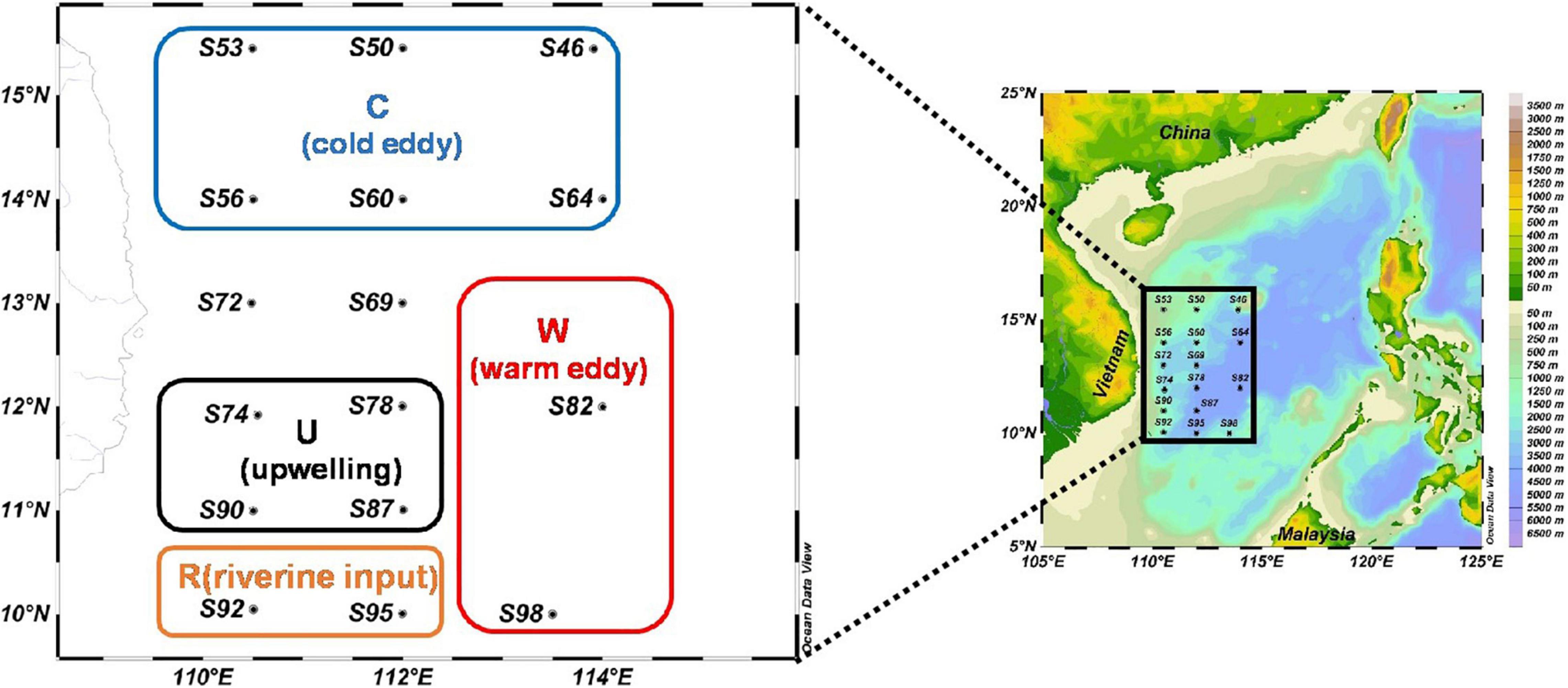
Figure 1. The investigation map in the western South China Sea (C: areas affected by cold eddy; W: areas affected by warm eddy; U: areas affected by upwelling; and R: areas affected by riverine input).
Sampling and Analysis
At each sampling station, the Seabird CTD was used to record the temperature, salinity, and fluorescence intensity of the seawater. Simultaneously, according to the fluorescence distribution, four layers (surface layer, maximum Chl-a layer, 100-m layer, and 200-m layer) were set, and 7-L seawater samples were collected from each layer, to determine Chl-a concentration, nutrient concentration, phytoplankton community, and phytoplankton sinking rate.
In this study, the concentration of Chl-a was determined by a fluorescence method (Welschmeyer, 1994). Two-liter seawater samples were filtered by GF/F film of 25 mm, and the filter film was kept under shading at −20°C. Chl-a was extracted in the dark with 90% acetone for 24 h at −20°C and measured with a Turner-Designs Trilogy TM fluorescence analyzer. Continuous Flow Auto Analyzer (Bran + Luebbe) was used to determine the concentration of nutrient such as NH4-N, NO3-N, PO4-P, SiO3-Si, and NO2-N in the laboratory (Liu et al., 2011). The structure of phytoplankton community was analyzed by the Utermöhl method (Sun et al., 2002). The identification of phytoplankton species taxa in the study area mainly referred to the article written by Sun et al. (2007). Cell volume conversion of phytoplankton was carried out according to the geometric model of cell volume (Sun and Liu, 2003). Carbon content and equivalent sphere diameter (ESD) of phytoplankton cells were converted according to cell volume (Eppley et al., 1970). The sinking rate of phytoplankton was determined by the SETCOL method (Bienfang, 1981). In order to acquire data with more credibility, four parallel water samples were set in each water layer, and each plexiglass column with a height of 0.53 m and a volume of 1,080 ml (Figure 2) was filled completely with a homogeneous seawater sample and capped. After sinking for 2 h, the water samples from one of the columns were collected in sequence from outlets 1, 2, and 3, the sinking rate of phytoplankton of each species was calculated in one column (red box), and the other three columns were used to calculate the total phytoplankton sinking rate.
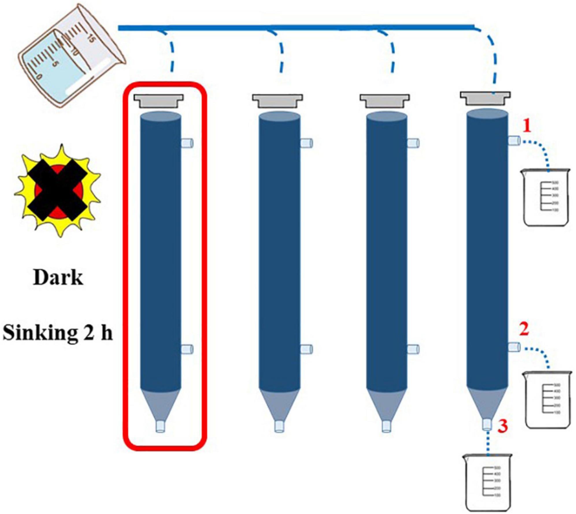
Figure 2. Application of SETCOL method in this study (Bienfang, 1981).
Data Analysis
The calculation formula of phytoplankton dominance (Y; Sun and Liu, 2004) is as follows:
where ni is the cell abundance of species i phytoplankton species in all samples, N is the cell abundance of all species, and fi is the frequency of occurrence for species i in all samples.
The sinking rates of phytoplankton is calculated as follows (Bienfang, 1981):
where ψ is sinking rate, Bs is the biomass settled into the bottom compartment, Bt is the total biomass in the column, L is the height of the column, and t is the settling interval.
Phytoplankton cell carbon and ESD were calculated by the following formula (Eppley, 1972):
where C is the carbon of per cell (pg C cell–1) and V is the cell biovolume of each species (μm).
The carbon flux (F) of phytoplankton is calculated according to the following formula:
where F is phytoplankton carbon flux, ψa is the average of the sedimentation rate in water column, and Ca is the average of the phytoplankton biomass carbon.
In this study, Ocean Data View was used to draw and analyze the location map of the sampling station and the temperature and salinity distribution map. The Chl-a distribution and phytoplankton community composition were plotted and analyzed by Origin 2016. SPSS14.0 software was used to analyze the correlation between phytoplankton sedimentation rate and environmental factors.
Results
Hydrographic Conditions of the Survey Area
The planar distribution of temperature, salinity, and nutrient (DIP: dissolved inorganic phosphorus; DIN: dissolved inorganic nitrogen; and DSi: dissolved inorganic silicate) at each water layer is shown in Figure 3. The temperature of the survey sea area ranged from 12.98 to 29.95°C (average = 21.38 ± 5.77°C; Figures 3A–D). The salinity ranged from 31.66 to 34.64 PSU (average = 34.20 ± 0.65 PSU; Figures 3E–H). In the north part of the survey area, an obvious area of low temperature and high salinity at shallow water above 100 m (blue box) proves that there had been a cold eddy in the survey area. In the middle of the survey sea area, the lowest temperature and the highest salinity of each water layer were found (blank box). Combined with the previous studies, it can be proved that it was an upwelling region (Wu and Li, 2003; Xie et al., 2003; Hu and Wang, 2016). In the eastern part of the sea area, an area of high temperature and low salinity was found between the DCM layer and the 100-m layer (red box), which proved that a warm eddy occurred here. At the bottom of the survey area, high temperature and low salt surface water appeared (orange box), indicating that this area was heavily affected by riverine input water.
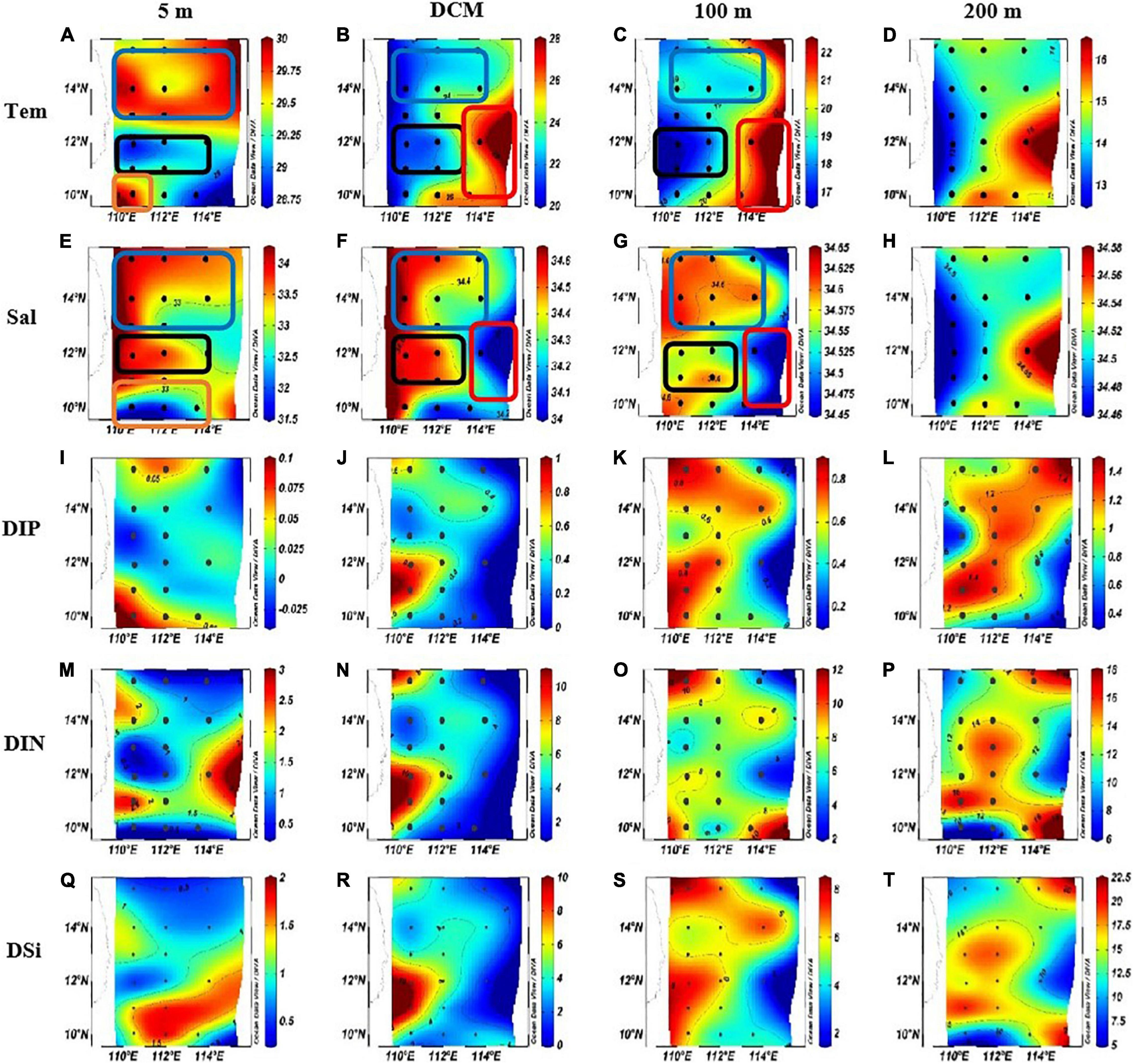
Figure 3. The horizontal distributions of temperature (Tem) (°C), Salinity (Sal) and nutrient concentration in the western South China Sea in autumn 2016. (A) Surface temperature. (B) DCM layer temperature. (C) 100 m layer temperature. (D) 200 m layer temperature. (E) Surface salinity. (F) DCM layer salinity. (G) 100 m layer salinity. (H) 200 m layer salinity. (I) surface DIP concentration. (J) DCM layer DIP concentration. (K) 100 m layer DIP concentration. (L) 200 m layer DIP concentration. (M) Surface DIN concentration. (N) DCM layer DIN concentration. (O) 100 m layer DIN concentration. (P) 200 m layer DIN concentration. (Q) Surface DSi concentration. (R) DCM layer DSi concentration. (S) 100 m layer DSi concentration. (T) 200 m layer DSi concentration.
The concentration of DIP, DIN, and DSi varied from 0 to 1.48 μmol L–1 (average = 0.52 ± 0.43 μmol L–1; Figures 3I–L), 0.26–17.98 μmol L–1 (average = 6.52 ± 4.90 μmol L–1; Figures 3M–P), and 0.44–20.44 μmol L–1 (average = 6.36 ± 5.58 μmol L–1; Figures 3Q–T), respectively. In addition to the surface layer, the concentration distribution of nutrients in other water layers is similar in response to mesoscale physical processes: in the cold eddy area and the upwelling area, the concentration of all kinds of nutrients was high; in the warm eddy region, the nutrient concentration was low. In the surface seawater, the DIP concentration was higher in the riverine input area and the cold eddy area, while the concentration in other areas was lower; DIN concentration was lower in the cold eddy area, the upwelling area, and the dilute water area; and the concentration of DSi was lower in the cold eddy region and the upwelling region, while it was higher in the warm eddy region.
The Distribution of Chlorophyll a and the Phytoplankton Community Structure
Through microscopic examination of the samples in the wSCS in the autumn of 2016, a total of 108 phytoplankton species were identified belonging to 54 genera from the samples collected in the present investigation, including 50 species of Bacillariophyta, 54 species of Dinophyta, 3 species of Cyanophyta, and 1 species of Chrysophyta. Bacillariophyta and Dinophyta were the main phytoplankton communities in the investigated sea area, whose species number accounts for 96% of the total phytoplankton species. The dominant phytoplankton species in the sea area are shown in Table 1. The most dominant species was Trichodesmium thiebautii. After removing all cyanobacteria, the dominance of Coscinodiscus argus was significantly higher than other species, accounting for 31% of the total phytoplankton cell abundance.
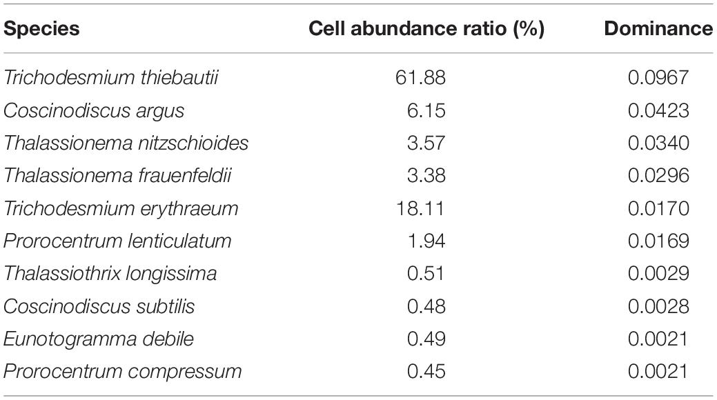
Table 1. Dominant species in the western South China Sea in autumn 2016.
In order to intuitively compare the effects of mesoscale physical processes on phytoplankton abundance and community distribution, the stations were divided into five regions: region C affected by cold eddy (S46, S50, S53, S56, S60, and S64); region U affected by upwelling (S74, S78, S87, and S90); region W affected by warm eddy (S82 and S98); region R affected by riverine input (S92 and S95); and others that were not affected by mesoscale physical process. The concentration of Chl-a and the distribution of phytoplankton cell abundance at each station in the investigated sea area are shown in Figure 4. The variation range of Chl-a concentration was 0.003–0.666 μg L–1, with an average value of 0.117 μg L–1. The concentration of Chl-a has little correlation with the abundance of phytoplankton cells, which may be related to the different phytoplankton species in each water layer after the influence of mesoscale physical processes. The cell abundance of T. thiebautii had no significant contribution to the concentration of Chl-a. For example, in the surface layer of S95 and the DCM layer of S69, T. thiebautii account for 96.0 and 98.3% of the total cell abundance, respectively, but the concentration of Chl-a was below the other stations. The cell abundance of diatom directly affected the concentration of Chl-a. In this study, it was found that the concentration of Chl-a in the DCM layer was always high in the station with high abundance of C. argus, such as S90 and S64.
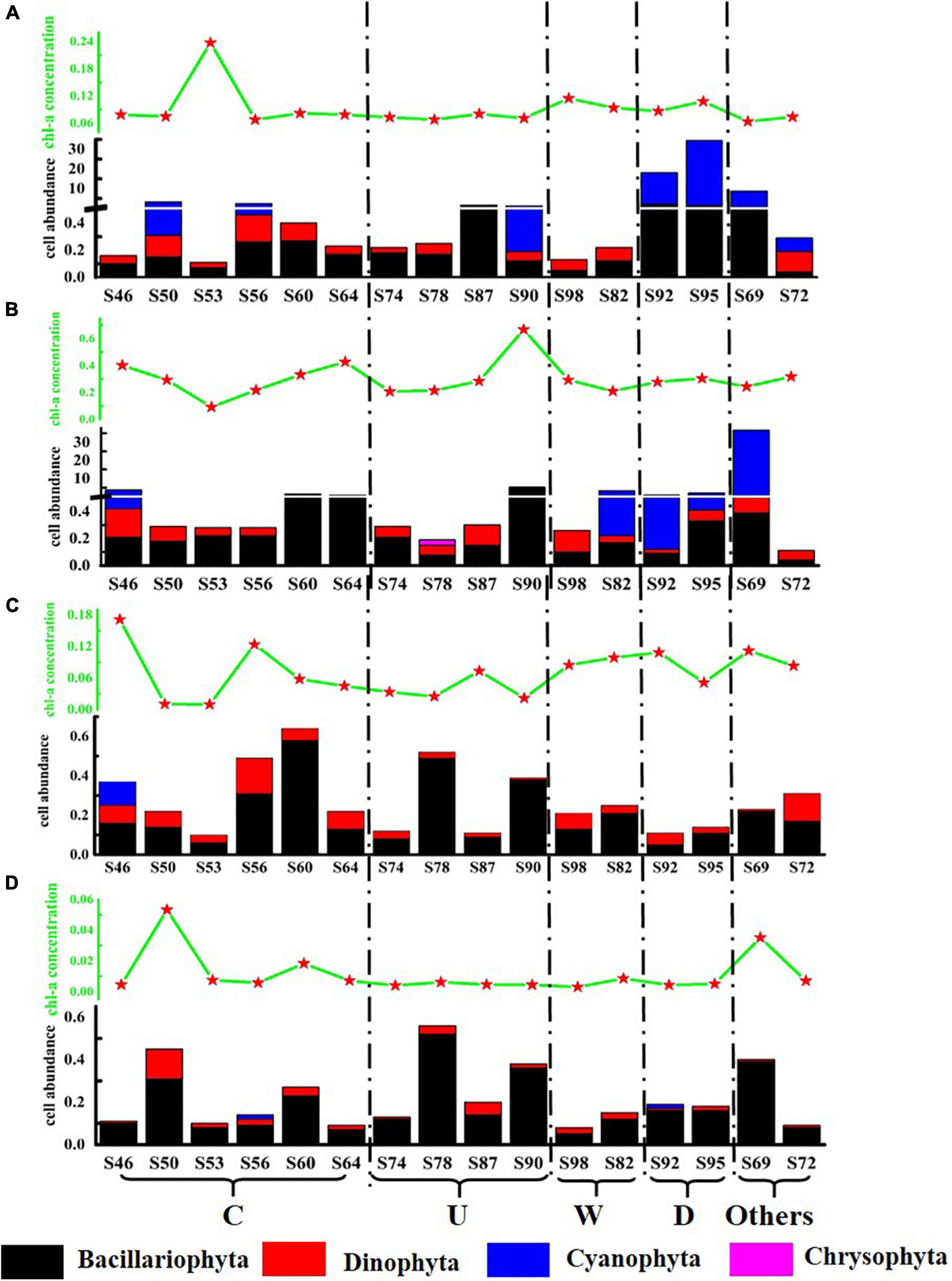
Figure 4. Schematic diagram of Chl-a concentration (μg L–1) and phytoplankton cell abundance (cell L–1) at the survey station in the western South China Sea in autumn 2016. (A) 5 m layer; (B) DCM layer; (C) 100 m layer; and (D) 200 m layer.
Both the cold eddy and upwelling brought the deep cold water to the upper layer. Because each station had a different effect, in this study, according to the distribution of temperature and salinity, the most influential stations were selected for analysis. The most affected station in the cold eddy area was S53, in which the cell abundance of diatom increased significantly. The most affected stations in the upwelling area were S90 and S87; the cell abundance of diatom was significantly increased. The rise in cell abundance of diatom is caused by the cold eddy and upwelling, in which the main species was C. argus. As a result of warm eddy, T. thiebautii in the surface layer was brought to the DCM layer at S82. The surface seawater of S92 and S95 was affected by fresh water, and the cell abundance was significantly higher than the other stations, among which T. thiebautii is greatly abundant. It was preliminarily concluded that the fresher water brought the extreme abundance of T. thiebautii.
Carbon Biomass of Phytoplankton
The carbon biomass of dominant phytoplankton species and other species in the survey area is shown in Figure 5. The variation range of phytoplankton carbon biomass was 4.36 × 10⁻⁵–0.07 mg C L–1, and the mean value was 0.002 mg C L–1. The largest phytoplankton carbon biomass was in the DCM layer, and most of the phytoplankton carbon biomass were contributed by C. argus. In region C and region U, it can be seen that C. argus has the least contribution to the carbon biomass in the surface layer and has a great contribution in the DCM layer and 100-m layer. According to the formula in section “Sampling and analysis,” the ESD of C. argus is about 58.294 μm. Compared with other dominant species, C. argus is larger in size and does not have characteristics that can resist sedimentation, so it can easily live in the DCM layer and deeper water layer. In this study, it was found that cold eddy and upwelling could bring the deep sea water that is rich in C. argus to the surface, and C. argus only stayed on the surface for a short time and then continued to sink to the DCM layer or deeper layers. Warm eddy brought phytoplankton from the surface to the deep water, leading to the increase of carbon biomass in the deep water. The riverine input brought a high abundance of cyanobacteria from the river to the ocean, leading to the highest carbon biomass in the surface water.
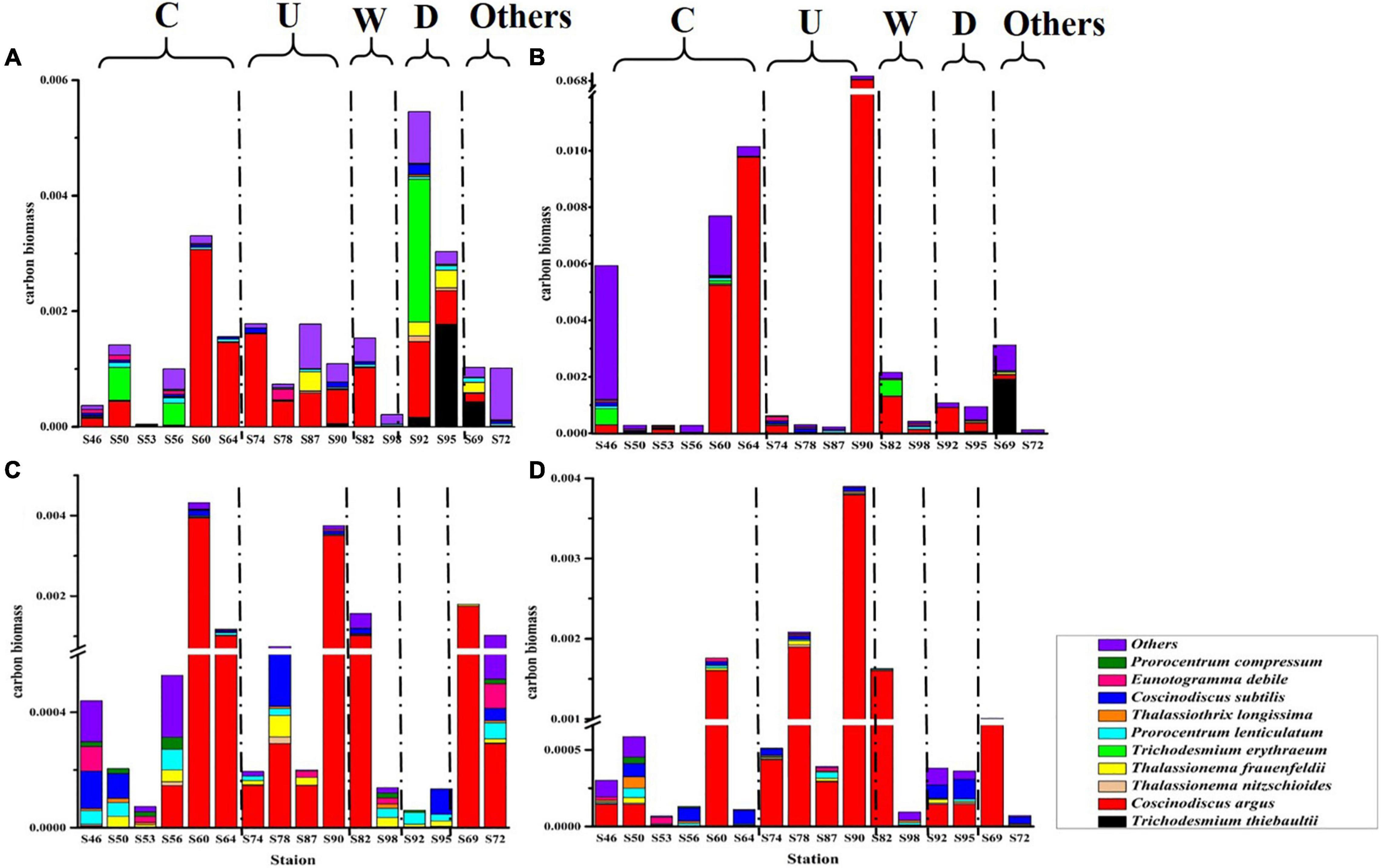
Figure 5. The carbon biomass (mg C L–1) of phytoplankton at the survey station in the western South China Sea in autumn 2016. (A) 5 m layer; (B) DCM layer; (C) 100 m layer; and (D) 200 m layer.
Sinking Rate of Phytoplankton
The sinking rate of phytoplankton is shown in Figure 6. The range of the sinking rate of phytoplankton was 0.12–3.17 m day–1, and the average value was 0.72 m day–1. The sedimentation rate of phytoplankton was highest in the 200-m layer and relatively low in all other three water layers. The sedimentation rate of phytoplankton is governed by multiple factors. In this study, we found that various mesoscale physical processes in the marine area and the cell abundance of C. argus had the most significant effects on the sedimentation rate. What is more, different mesoscale physical processes affect the sedimentation rate by influencing the phytoplankton community distribution. The sinking rate of the DCM water layer at S60 and S64 in region C was relatively high, and the percentage of C. argus in diatom was 52.9 and 87%, respectively. Similarly, the sinking rate was the highest at S90 in region U, and the C. argus proportion of diatom in the DCM layer was 93%. The sinking rate of region W was relatively low in the surface layer to the 100-m layer, mainly because the warm eddy brought the surface sea water and active surface phytoplankton to the deep layer, which was caused by the upward movement of phytoplankton. The surface seawater of region R contains abundant phytoplankton, which were obtained from the riverine input, leading to the high sinking rate.
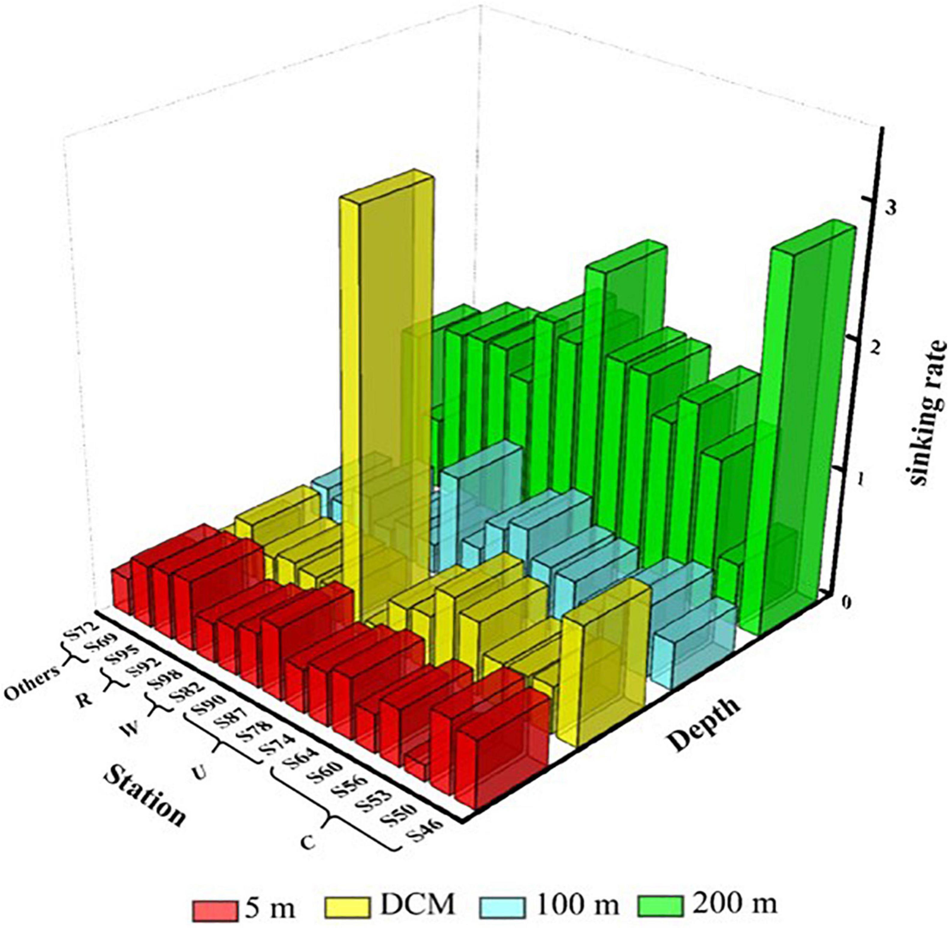
Figure 6. Sinking rate (m day–1) of phytoplankton at the survey station in the western South China Sea in autumn 2016.
Carbon Flux of Phytoplankton
The vertical distribution of phytoplankton carbon flux in the surveyed sea area is shown in Figure 7. The carbon flux of phytoplankton could directly represent the contribution of phytoplankton to carbon in each water layer. The variation range of phytoplankton carbon flux was 2.41 × 10⁻⁶–0.006 mg C m–2 day–1, and the average value was 0.0002 mg C m–2 day–1. Cold eddy and upwelling caused the carbon flux values of phytoplankton in the DCM layer to increase, with the most pronounced performance at station S90. Warm eddy caused lower carbon flux in all phytoplankton layers, as represented by station S98. The riverine input of fresh water caused the carbon flux of surface phytoplankton to increase, highlighted at station S92 (Figure 7A). Phytoplankton carbon flux was highest in the 200-m layer, followed by the DCM layer, and lowest in the 100-m layer (Figure 7B).
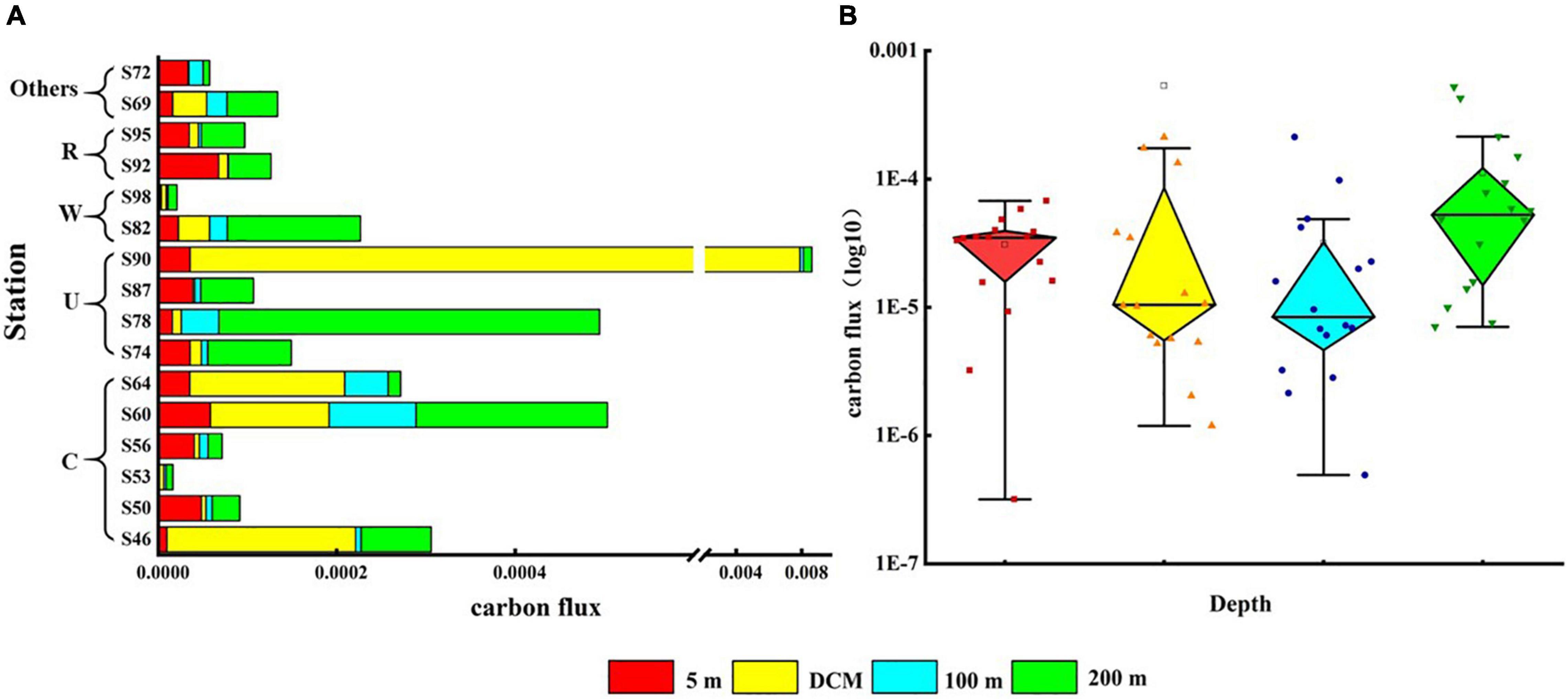
Figure 7. Carbon flux (mg C m–2 day–1) of phytoplankton at the survey station in the western South China Sea in autumn 2016. (A) Phytoplankton carbon flux in each water layer under various mesoscale physical processes; (B) summary of phytoplankton carbon flux at each station in four water layers.
Discussion
The Sinking Rate of Phytoplankton and Its Controlling Environmental Factors
The correlation analysis results between the sinking rate of phytoplankton and the environmental factors in each water layer of the investigated sea area are shown in Figure 8. It has been found that the sinking rate of phytoplankton measured in the laboratory was mainly determined by environmental parameters (Bienfang, 1984; Johnson and Smith, 1986; Muggli et al., 1996; Pantorno et al., 2013). Different from the previous research, the results of this study showed that the sinking rate of phytoplankton was not significantly correlated with most environmental factors especially nutrient concentrations, which was similar to the research results of Guo et al. (2016). The sinking rate of phytoplankton in the 100-m water layer had a significant negative correlation with temperature, while the partial nutrient concentration in the DCM layer and 100-m layer had a positive effect on the sinking rate. In laboratory experiments, phytoplankton lived in a stable hydrological environment, and the sinking rate was greatly affected by environmental factors. However, due to the interaction of various mesoscale physical processes, the environmental parameters in the investigated sea area were changeable, so the environmental parameters had little influence on phytoplankton in the field experiment.
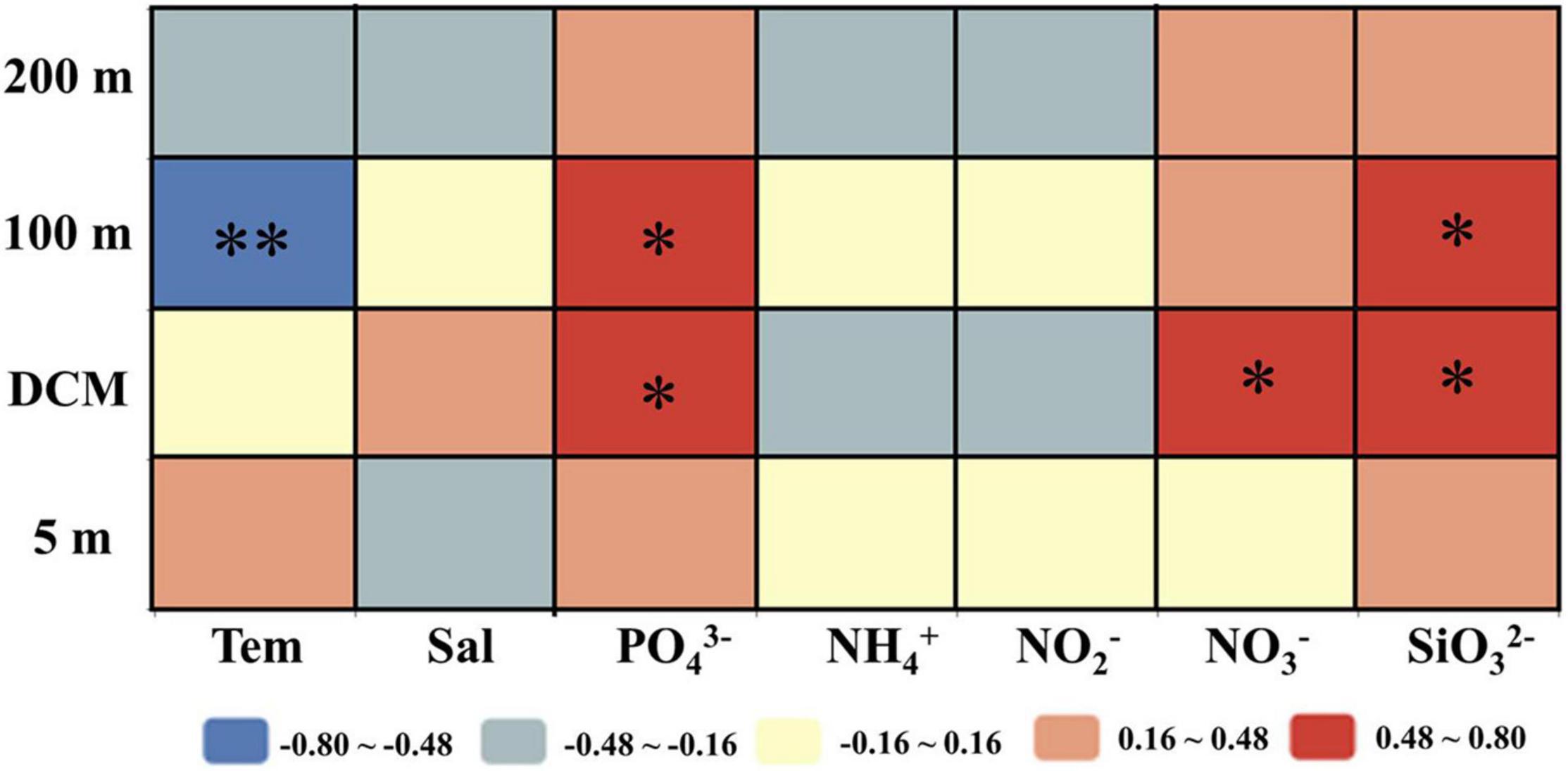
Figure 8. Relationships between phytoplankton sinking rate and environmental parameters in the survey area in the western South China Sea in autumn 2016. Pearson correlation coefficients (r) ranged from negative to positive and are indicated by color intensity changing from dark blue to red, respectively. **p < 0.01; *p < 0.05 (two-tailed). Tem: Temperature; Sal: Salinity; PO43–, NH4+, NO2–, NO3–, SiO32–: concentration of each component.
The Sinking Rate of Dominant Phytoplankton Species
The sinking rate of phytoplankton was affected by many factors. In order to explore whether cell morphology has a significant effect on the sinking rate of phytoplankton, the first 20 dominant species were selected to compare their cell ESD, direct measurement sinking velocity, and real specific vertical flux of a single species (Table 2). The sinking rate of phytoplankton was correlated with community structure (Culver and Smith, 1989). The sinking rate of Bacillariophyta was generally higher than that of Dinophyta, while that of Cyanophyta was the lowest. According to Stokes’ law, both cell size and cell density were important factors to determining the sinking rate. As shown in Figure 9, there was no significant correlation between the sinking rate of phytoplankton and its own cell size, which indicated that the cell density of phytoplankton had a greater influence on the sinking rate. Culver and Smith (1989) and Muggli et al. (1996) found that the sinking rate of phytoplankton cells was related to the physiological activity of the cells. Many studies had shown that the impact of water flow on phytoplankton was also extremely important. The scientists believed that water disturbance could reduce the precipitation rate of phytoplankton (Walsby and Reynolds, 1980; Lande and Wood, 1987); Other scientists suggested that water disturbance would accelerate the rate of phytoplankton deposition (Ruiz et al., 1996, 2004). Therefore, it is not enough to research the sinking rate of phytoplankton in the whole sea area by a single factor. More detailed studies on phytoplankton sinking rate should be carried out from various perspectives, such as phytoplankton cell density, cell physiological activity measurement, and sea water characteristics.
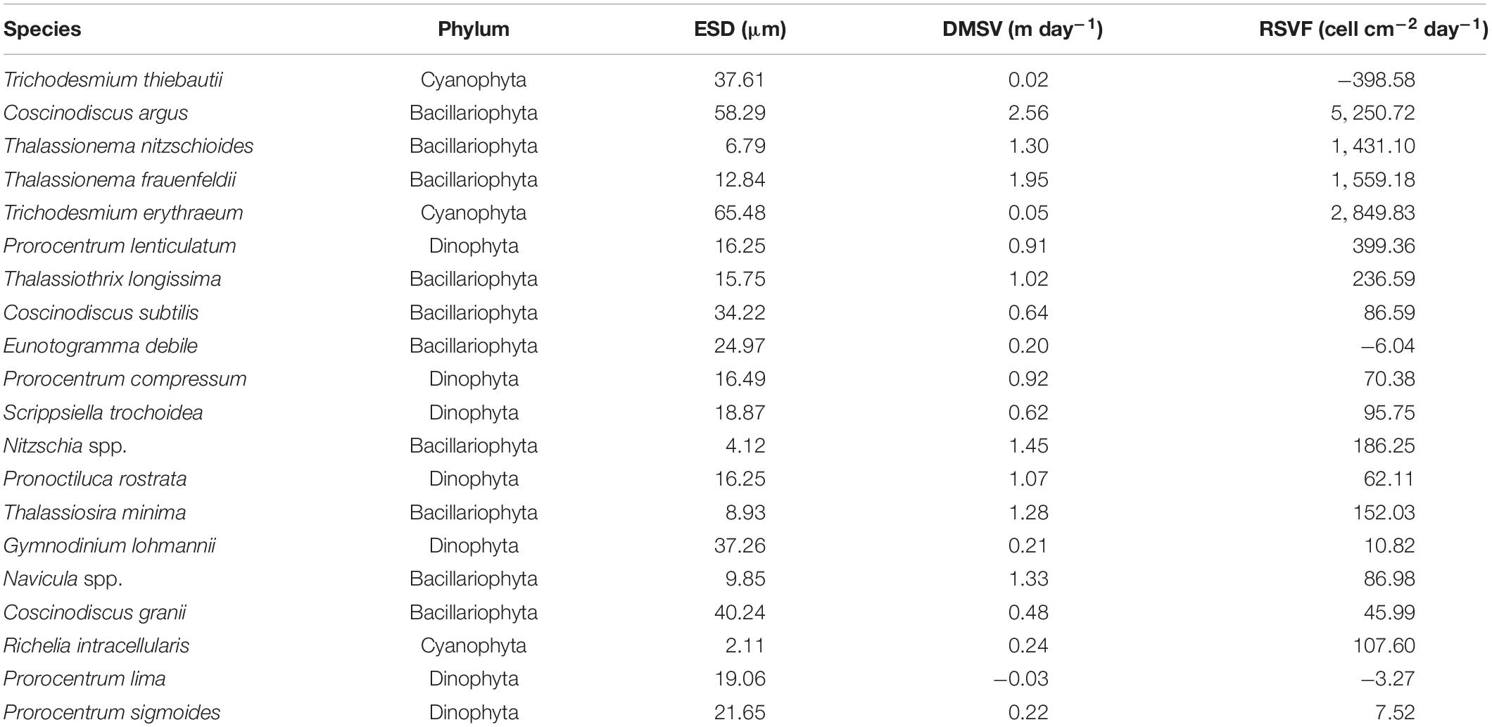
Table 2. The equivalent spherical diameter (ESD), direct measurement sinking velocity (DMSV), and real specific vertical flux (RSVF) of the first 20 phytoplankton taxa in the survey area in the western South China Sea in autumn 2016.
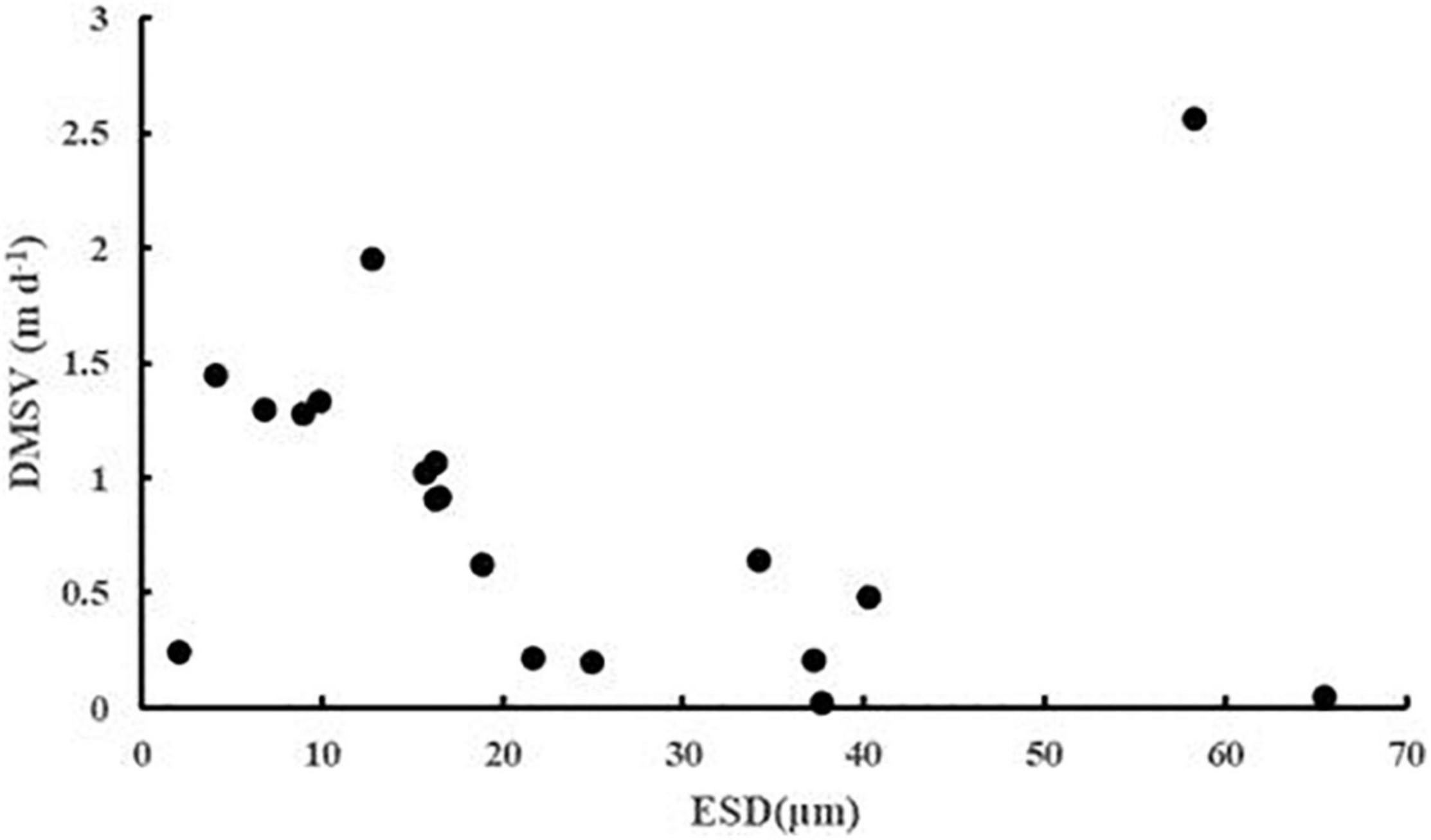
Figure 9. The ESD (μm) and DMSV (m day–1) scatter plots of the first 20 phytoplankton taxa in the survey area in the western South China Sea in autumn 2016.
Response of the Sinking Rate to Mesoscale Physical Processes
The SCS, which is located between the Indian monsoon and Asian monsoon region, is subject to seasonal risk control all year round, resulting in a multi-eddy structure (Wyrtki, 1961; Chen and Yang, 2010). Owing to the strong vertical stratification throughout the SCS, the growth of surface phytoplankton is limited by nutrient concentrations (Ning et al., 2004). Hence, the generation and reduction of numerous eddies can vary the amount of nutrients entering the euphotic layer and play an important role in the growth and distribution of phytoplankton (McGillicuddy et al., 2003; Lin et al., 2010; He et al., 2019). During the summer, an offshore rapid flow from the southwest to the northeast usually forms at about 12°N in the eastern part of Vietnam due to the influence of the southeast monsoon, which transports the cold water masses generated by the coastal upwelling to the basin area (Xie et al., 2003; Liang and Tang, 2017). The rapids are part of a cold–warm eddy dipole structure in the western part of the SCS during summer, located between the cold and warm eddies (Wang et al., 2006; Gan and Qu, 2008). The northern part of the rapids is frequently subjected to eruptive algal blooms into the basin, which explains the phytoplankton blooms in the western part of the SCS in summer (Tang et al., 2004a,b). The study of mesoscale physical processes has special significance for the development of ecology, chemistry, biology, and other disciplines. Therefore, mesoscale vortex plays a very important role in biogeochemistry.
The correlation findings obtained in this study can be briefly summarized in conjunction with Figure 10. Due to the influence of cold eddy, the nutrient concentration of each water layer was relatively higher; furthermore, the concentration of Chl-a in the DCM layer was the highest at all stations except S53, which caused the maximum Chl-a layer to move up. The cell abundance of Bacillariophyta was larger in the DCM layer and the 100-m layer; C. argus, Coscinodiscus subtilis, Thalassionema nitzschioides, and Thalassionema frauenfeldii accounted for a large proportion, while Dinophyta was larger in the 5-m layer and DCM layer, mainly dominated by Prorocentrum compressum and Prorocentrum lenticulatum. The sinking rate of phytoplankton was higher in the 200-m layer and the DCM layer, but decreased in the 5-m layer. It is worth noting that the C. argus with high abundance appeared in both S60 and S64, and their sinking rates were very high in the DCM layer. Influenced by the cold eddy, a large number of C. argus were carried to the upper sea water, leading to a faster sinking rate of phytoplankton in the DCM layer. Surface phytoplankton were mainly Prorocentrum brought by cold eddy, and due to sufficient illumination and abundant nutrients, their physiological state was more active and thus the sinking rate was slower. In the area affected by upwelling, the nutrient concentration of each water layer increased, and the concentration of Chl-a was the highest in the DCM layer, followed by the 5-m layer. The cell abundance of Bacillariophyta at all stations except S87 showed an increasing trend with the deepening of water layer, in which the main species were T. nitzschioides, T. frauenfeldii, and C. argus. S87 showed the highest abundances in the 5-m layer; however, the dominant species were still T. nitzschioides and T. frauenfeldii. This is mainly due to the two species with high abundances at S87 that existed in single branches examined under the microscope, while at other stations, they existed in bunches or clusters; this form could not be easily carried to the upper seawater, such that the abundances increased in the deeper layers. The response to the upwelling was the most significant at S90, the C. argus cell abundance in this station was absolutely dominant, and the sinking rate was the highest at the DCM layer, reaching 3.17 m day–1. Generally speaking, the upwelling was associated with the cold eddy (Chai et al., 2001), and the high cell abundance of individual diatom species (such as C. argus) and the high phytoplankton sinking rate in the DCM layer in the study area were mainly affected by the cold eddy and the upwelling. It is inferred that there may be a connection between the abnormally high values of C. argus and the algal blooms formed by the rapids. In the area affected by the warm eddy, the concentration of nutrient in each water layer was decreased. The effect of warm eddy on Chl-a concentration was not obvious; the DCM layer was the largest, and the 200-m layer was the lowest. The cell abundance of Bacillariophyta at the 100-m layer was the largest, mainly of T. nitzschioides and T. frauenfeldii, while the cell abundance of Dinophyta at the 5-m layer and DCM layer was the largest, mainly of P. lenticulatum. Cyanophyta only appeared in the DCM layer. This means that warm eddy carried Bacillariophyta and Cyanophyta from the upper layer to the deeper water, and Dinophyta were still distributed in the upper layer because they could move by themselves. The influence of warm eddy on phytoplankton sinking rate was mainly reflected in the surface layer, while the values of sedimentation rate in the DCM and 100-m layer were lower and minimized in the DCM layer. This is mainly caused by the upward movement of phytoplankton as warm eddy carries the phytoplankton from the surface to deeper layers. Part of the sea area under investigation was affected by the fresh water, resulting in a high abundance of phytoplankton species and quantities in the surface layer and an increase in the number of dinoflagellate in the DCM layer, mainly Prorocentrum and Gymnodinium. The sinking rate in the surface layer was higher than that in the DCM layer and 100-m layer.
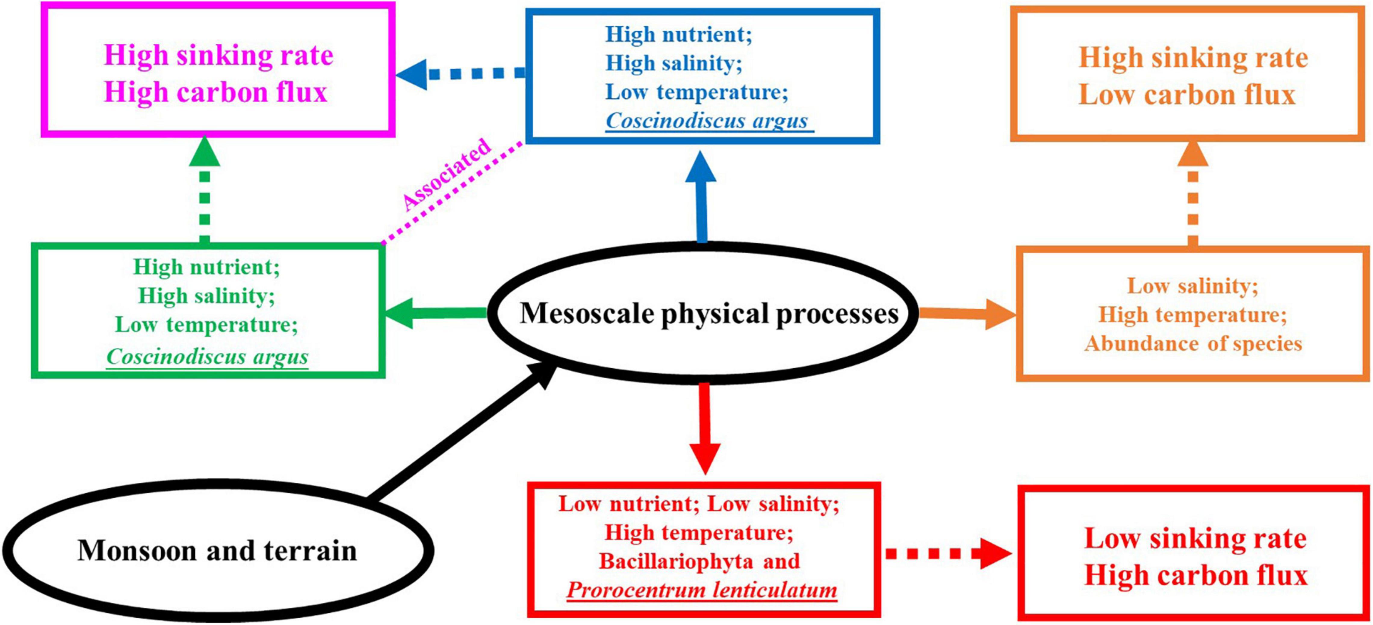
Figure 10. A conceptual schematic for the phytoplankton community and the sinking rate response to mesoscale physical processes (the blue solid line represents cold eddy, the green represents upwelling, the red represents warm eddy, and the orange represents riverine input water).
Final Conclusion
There were many kinds of mesoscale vortices in the investigated sea area, and their effects on phytoplankton community and sinking rate were significant. The sinking rate of the DCM layer increased due to the cold vortex and the upwelling, and the response of C. argus was the largest. Warm eddy could reduce the sinking rate of phytoplankton in shallow water above 100 m. The carbon flux of phytoplankton showed that the bottom layer had the largest carbon flux, followed by the DCM layer, and the 100-m layer was the smallest, which could be well explained by the sinking rate of phytoplankton. The faster the sinking rate was, the greater the carbon flux contributed by phytoplankton. The division of mesoscale physical process regions in this study is mainly based on the in situ temperature and salinity data and the results of previous studies, but there is a lack of investigation and research related to the rapids in the sea area. Moreover, the sinking rate obtained in the experiment is only a relatively rough value, without considering the direction and velocity of the eddies in the sea area, which can still reflect the response of the phytoplankton community structure and sinking rate to the mesoscale physical processes. It was expected to provide basic data to study the response of phytoplankton sinking rate to mesoscale vortices in the SCS, and more accurate and specific studies are needed in the future.
Data Availability Statement
The original contributions presented in the study are included in the article/supplementary material, further inquiries can be directed to the corresponding author/s.
Author Contributions
JS designed the experiment. YM, YL, and GQ collected the samples. YM, XL, and YL performed the sample analysis. YM and JS wrote the manuscript, with contribution from all authors. All authors read and approved the final manuscript.
Funding
This research was financially supported by State Key Laboratory of Biogeology and Environmental Geology, China University of Geosciences (No. GKZ21Y645), the National Nature Science Foundation of China grants (41876134, 41676112, and 41276124), and the Changjiang Scholar Program of Chinese Ministry of Education (T2014253) to JS.
Conflict of Interest
The authors declare that the research was conducted in the absence of any commercial or financial relationships that could be construed as a potential conflict of interest.
Publisher’s Note
All claims expressed in this article are solely those of the authors and do not necessarily represent those of their affiliated organizations, or those of the publisher, the editors and the reviewers. Any product that may be evaluated in this article, or claim that may be made by its manufacturer, is not guaranteed or endorsed by the publisher.
Acknowledgments
We would like to thank the Open Cruise Project in western South China Sea of National Nature Science Foundation of China (NORC2016-07) for sharing their ship time. We are also extremely grateful to the research team led by researcher Jie Xu from the South China Sea Institute of Oceanology Chinese Academy of Sciences for providing the sea area temperature and salinity data.
References
Behrenfeld, M. J. (2014). Climate – mediated dance of the plankton. Nat. Clim. Chang. 10, 880–887. doi: 10.1038/nclimate2349
Behrenfeld, M. J., Hu, Y. X., Malley, R. T., Boss, E. S., Hostetler, C. A., Siegel, D. A., et al. (2017). Annual boom – bust cycles of polar phytoplankton biomass revealed by space – based lidar. Nat. Geosci. 10, 118–122. doi: 10.1038/ngeo2861
Bienfang, P. K. (1981). SETCOL – a technologically simple and reliable method for measuring phytoplankton sinking rates. Can. J. Fish. Aquat. Sci. 38, 1289–1294. doi: 10.1139/f81-173
Bienfang, P. K. (1984). Size structure and sedimentation of biogenic microparticulates in a subarctic ecosystem. J. Plankton Res. 6, 985–995. doi: 10.1093/plankt/6.6.985
Bienfang, P. K. (1985). Size structure and sinking rates of various microparticulate constituents in oligotrophic Hawaiian waters. Mar. Ecol. Prog. Ser. 23, 143–151. doi: 10.3354/meps023143
Boyd, P. W., and Newton, P. P. (1999). Does planktonic community structure determine downward particulate organic carbon flux in different oceanic provinces? Deep Sea Res. Part I 46, 63–91. doi: 10.1016/S0967-0637(98)00066-1
Chai, F., Xue, H. J., and Shi, M. C. (2001). Formation and distribution of upwelling and downwelling in the South China Sea. Oceanogr. China 13, 117–128.
Chen, Q. Y., and Yang, K. D. (2010). Mean square deviation analysis of the sea surface temperature interannual variability in the South China Sea. Audio Eng. 34, 72–75. doi: 10.16311/j.audioe.2010.11.001
Culver, M. E., and Smith, W. O. (1989). Effects of environmental variation on sinking rates of marine phytoplankton. Phycology 25, 262–270. doi: 10.1111/j.1529-8817.1989.tb00122.x
Eppley, R. W., Holmes, R. W., and Strickland, J. D. H. (1967). Sinking rates of marine phytoplankton measured with a fluorometer. J. Exp. Mar. Biol. Ecol. 1, 191–208. doi: 10.1016/0022-0981(67)90014-7
Eppley, R. W., Reid, F. M. H., and Stickland, J. D. H. (1970). Estimates of phytoplankton crop size, growth rate and primary production. Bull. Scripps Inst. Oceanogr. Univ. Cal. 17, 33–42.
Fang, W. D., Fang, G. H., Shi, P., Huang, Q. Z., and Xie, Q. (2002). Seasonal structures of upper layer circulation in the southern South China Sea from in situ observations. J. Geophys. Res. Oceans 107, 23-1-23-12. doi: 10.1029/2002JC001343
Gan, J. P., and Qu, T. D. (2008). Coastal jet separation and associated flow variability in the southwest South China Sea. Deep Sea Res. Part I 55, 1–19. doi: 10.1016/j.dsr.2007.09.008
Guan, B. X., and Yuan, Y. C. (2006). Overview of studies on some eddies in the China seas and their adjacent seas I. The South China Sea and the region east of Taiwan. Acta Oceanol. Sin. 8, 1–16. doi: 10.3321/j.issn:0253-4193.2006.03.001
Guo, S. J., Sun, J., Zhao, Q. B., Feng, Y. Y., Huang, D. J., and Liu, S. M. (2016). Sinking rates of phytoplankton in the Changjiang (Yangtze River) estuary: a comparative study between Prorocentrum dentatum and Skeletonema dorhnii bloom. J. Mar. Syst. 154, 5–14. doi: 10.1016/j.jmarsys.2015.07.003
He, Q. Y., Zhan, H. Z., Xu, J., Cai, S. Q., Zhan, W. K., Zhou, L. B., et al. (2019). Eddy-induced chlorophyll anomalies in the Western South China Sea. J. Geophys. Res. Oceans 124, 9487–9506. doi: 10.1029/2019JC015371
Hu, J. Y., and Wang, X. H. (2016). Progress on upwelling studies in the China seas. Rev. Geophys. 54, 653–673. doi: 10.1002/2015RG000505
Hutchins, D. A., and Boyd, P. W. (2016). Marine phytoplankton and the changing ocean iron cycle. Nat. Clim. Chang. 6, 1072–1079. doi: 10.1038/nclimate3147
Johnson, T. O., and Smith, W. O. (1986). Sinking rates of phytoplankton assemblages in the Wedell Sea marginal ice zone. Mar. Ecol. Prog. Ser. 33, 131–137. doi: 10.3354/meps033131
Kromkamp, J., and Mur, L. (1984). Buoyant density changes the cyanobacterium aeruginosa due to changes in the cellular carbohydrate content. FEMS Microb. Lett. 25, 105–109. doi: 10.1016/0378-1097(84)90055-7
Lande, R., and Wood, A. M. (1987). Suspension times of particles in the upper ocean. Deep Sea Res. 34, 61–72. doi: 10.1016/0198-0149(87)90122-1
Leng, X. Y., Yang, Y., and Sun, J. (2016). Mesoscale physical processes on the effects of distribution of nutrients and chlorophyll-a in the western South China Sea in summer. Acta Oceanol. Sin. 4, 66–75. doi: 10.3969/j.issn.0253-4193.2016.04.006
Liang, W. Z., and Tang, D. L. (2017). Distribution characteristics of phytoplankton size structure in the western South China Sea in summer. J. Trop. Oceanogr. 36, 93–101.
Liao, C. H., Lee, K. T., Lee, M. A., and Lu, H. J. (1999). Biomass distribution and zooplankton composition of the sound-scattering layer in the waters of southern East China Sea. ICES J. Mar. Sci. 56, 766–778. doi: 10.1006/jmsc.1999.0497
Lin, I. I., Lien, C. C., Wu, C. R., Wong George, T. F., and Huang, C. W. (2010). Enhanced primary production in the oligotrophic South China Sea by eddy injection in spring. Geophys. Res. Lett. 37:L16602. doi: 10.1029/2010GL043872
Liu, S. M., Li, R. H., Zhang, G. L., Wang, D. R., and Du, J. Z. (2011). The impact of anthropogenic activities on nutrient dynamics in the tropical Wenchanghe and Wenjiaohe Estuary and Lagoon system in East Hainan. China Mar. Chem. 125, 49–68. doi: 10.1016/j.marchem.2011.02.003
Lu, Z. M., Gan, J. P., Dai, M. H., and Anson, Y. Y. C. (2010). The influence of coastal upwelling and a river plume on the subsurface chlorophyll maximum over the shelf of the northeastern South China Sea. J. Mar. Syst. 82, 35–46. doi: 10.1016/j.jmarsys.2010.03.002
McGillicuddy, D. J., Anderson, L. A., Doney, S. C., and Maltrud, M. E. (2003). Eddy-driven sources and sinks of nutrients in the upper ocean: results from a 0.1 degrees resolution model of the North Atlantic. Glob. Biogeochem. Cycles 17:1035. doi: 10.1029/2002GB001987
Muggli, D. L., Lecourt, M., and Harrison, P. J. (1996). Effects of iron and nitrogen source on the sinking rate, physiology and metal composition of an oceanic diatom from the subarctic Pacifific. Mar. Ecol. Prog. Ser. 132, 215–227. doi: 10.3354/meps130255
Ning, X., Chai, F., Xue, H., Chai, Y., Liu, C., and Shi, J. (2004). Physical-biological oceanographic coupling influencing phytoplankton and primary production in the South China Sea. J. Geophys. Res. Oceans 109:C10005. doi: 10.1029/2005JC002968
Pantorno, A., Holland, D. P., Stojkovic, S., and Beardall, J. (2013). Impacts of nitrogen limitation on the sinking rate of the coccolithophorid Emiliania huxleyi (Prymnesiophyceae). Phycologia 52, 288–294. doi: 10.2216/12-064.1
Peng, K. S. (2000). China water resource crisis in the 21th century. Adv. Sci. Technol. Water Resour. 20, 13–16. doi: 10.3880/j.issn.1006-7647.2000.05.005
Peperzak, L., Colijn, F., Koeman, R., Gieskes, W. W. C., and Joordens, J. C. A. (2003). Phytoplankton sinking rates in the Rhine region of freshwater influence. Plankton Res. 25, 365–383. doi: 10.1093/plankt/25.4.365
Pitcher, G. C., Walker, D. R., and Mitchell-Innes, B. A. (1989). Phytoplankton sinking rate dynamics in the southern Bengurla upwelling system. Mar. Ecol. Prog. Ser. 55, 261–269. doi: 10.3354/meps055261
Raymont, J. E. (2014). Plankton & Productivity in the Oceans: Volume 1: Phytoplankton. Amsterdam: Elsevier.
Reynolds, C. S. (1987). Cyanobacterial water blooms. Adv. Bot. Res. 13, 67–143. doi: 10.1016/S0065-2296(08)60341-9
Ruiz, J., Garcfa, M., and Rodriguez, J. (1996). Sedimentation loss of phytoplankton cells from the mixed layer: effects of turbulence levels. J. Plankton Res. 18, 1727–1734. doi: 10.1093/plankt/18.9.1727
Ruiz, J., Macias, D., and Peters, F. (2004). Turbulence increases the average settling velocity of phytoplankton cells. Proc. Natl. Acad. Sci. U.S.A. 101, 17720–17724. doi: 10.1073/pnas.0401539101
Shiah, F. K., Chung, S. W., Kao, S. J., Gong, G. C., and Liu, K. K. (2000). Biological and hydrographical responses to tropical cyclones (typhoons) in the continental shelf of the Taiwan Strait. Cont. Shelf Res. 20, 2029–2044. doi: 10.1016/S0278-4343(00)00055-8
Steele, J. H., and Yentsch, C. S. (1960). The vertical distribution of chlorophyll. J. Mar. Biol. Assoc. U.K. 39, 217–226. doi: 10.1017/S0025315400013266
Stokes, G. G. (1851). On the effect of internal friction of fluids on the motion of pendulums. Trans. Camb. Philos. Soc. 9, 8–14.
Su, J. L. (2004). Overview of the South China Sea circulation and its influence on the coastal physical oceanography outside the Pearl River Estuary. Cont. Shelf Res. 24, 1745–1760. doi: 10.1016/j.csr.2004.06.005
Sun, J. (2011). Marine phytoplankton and biological carbon sink. Acta Ecol. Sin. (in Chinese) 31, 5372–5378.
Sun, J., and Liu, D. Y. (2003). Geometric models for calculating cell biovolume and surface area for phytoplankton. J. Plankton Res. 25, 1331–1346. doi: 10.1093/plankt/fbg096
Sun, J., and Liu, D. Y. (2004). The application of diversity indices in marine phytoplankton studies. Acta Oceanol. Sin. (in Chinese) 26, 62–75. doi: 10.1088/1009-0630/6/5/011
Sun, J., Liu, D. Y., and Qian, S. B. (2002). A quantative research and analysis method for marine phytoplankton: an introduction to utermöhl method and its modification. J. Oceanogr. Huanghai Bohai Seas (in Chinese) 20, 105–112.
Sun, J., Song, S. Q., Le, F. F., Wang, D., Dai, M. H., and Ning, X. R. (2007). Phytoplankton in northern South China Sea in the winter of 2004. Acta Ecol. Sin. (in Chinese) 5, 132–145.
Tang, D. L., Kawamura, H., Doan-Nhu, H., and Takahashi, W. (2004a). Remote sensing oceanography of a harmful algal bloom off the coast of southeastern Vietnam. J. Geophys. Res. Oceans 109:C03014. doi: 10.1029/2003JC002045
Tang, D. L., Kawamura, H., Dien, T. V., and Lee, M. A. (2004b). Offshore phytoplankton biomass increase and its oceanographic causes in the South China Sea. Mar. Ecol. Prog. Ser. 268, 31–41. doi: 10.3354/meps268031
Titman, D., and Kilham, P. (1976). Sinking in freshwater phytoplankton: some ecological implications of cell nutrient status and physical mixing processes. Limnol. Oceanogr. 21, 409–417.
Walsby, A. E., and Reynolds, C. S. (1980). “Sinking and floating,” in The Physiological Ecology of Phytoplankton, ed. I. Morris (Oxford: Blackwell), 371–412.
Wang, G. H., Chen, D. K., and Su, J. L. (2006). Generation and life cycle of the dipole in the South China Sea summer circulation. J. Geophys. Res. Oceans 111:C06002. doi: 10.1029/2005JC003314
Welschmeyer, N. A. (1994). Fluorometric analysis of chlorophyll-a in the presence of chlorophyll-b and pheopigments. Limnol. Oceanogr. 39, 1985–1992. doi: 10.4319/lo.1994.39.8.1985
Wu, R. S., Guo, X. G., and Li, L. (2002). Winter hydrographic condition and circulation of the South China Sea. Acta Ecol. Sin. (in Chinese) 24(Suppl), 142–153.
Wu, R. S., and Li, L. (2003). Summarization of study on upwellings system in the South China Sea. J. Oceanogr. Taiwan Strait 22, 269–277. doi: 10.1007/BF02860423
Wu, X., Wang, H., Bi, N., Song, Z., Zang, Z., and Kineke, G. C. (2016). Bio-physical changes in the coastal ocean triggered by typhoon: a case of Typhoon Meari in summer 2011. Estuar. Coast. Shelf Science. 183, 413–421. doi: 10.1016/j.ecss.2016.04.014
Wyrtki, K. (1961). Physical oceanography of the Southeast Asian waters: scientific results of marine investigations of the South China Sea and the Gulf of Thailand. Naga Rep. 2:195.
Xie, S. P., Xie, Q., Wang, D. X., and Liu, W. T. (2003). Summer upwelling in the South China Sea and its role in regional climate variations. J. Geophys. Res. Earth Surf. 108:3261.
Xue, H. J., Cai, F., and Xu, J. P. (2001). Numerical calculation and Mesoscale characteristics of the South China Sea. Oceanogr. China 13, 48–89.
Zhong, C., Xiao, W. P., and Huang, B. Q. (2013). The response of phytoplankton to mesoscale eddies in western South China Sea. Adv. Mar. Sci. 31, 213–220. doi: 10.3969/j.issn.1671-6647.2013.02.007
Keywords: phytoplankton, community structure, sinking rate, South China Sea, mesoscale physical processes
Citation: Mao Y, Li X, Zhang G, Liao Y, Qian G and Sun J (2021) Sinking Rate and Community Structures of Autumn Phytoplankton Responses to Mesoscale Physical Processes in the Western South China Sea. Front. Microbiol. 12:777473. doi: 10.3389/fmicb.2021.777473
Received: 15 September 2021; Accepted: 28 October 2021;
Published: 06 December 2021.
Edited by:
Feixue Fu, University of Southern California, United StatesReviewed by:
Yantao Liang, Ocean University of China, ChinaMichael Thomas Montgomery, Texas A&M University Corpus Christi, United States
Copyright © 2021 Mao, Li, Zhang, Liao, Qian and Sun. This is an open-access article distributed under the terms of the Creative Commons Attribution License (CC BY). The use, distribution or reproduction in other forums is permitted, provided the original author(s) and the copyright owner(s) are credited and that the original publication in this journal is cited, in accordance with accepted academic practice. No use, distribution or reproduction is permitted which does not comply with these terms.
*Correspondence: Jun Sun, cGh5dG9wbGFua3RvbkAxNjMuY29t