

- 1 Department of Economics, National Chengchi University, Taipei, Taiwan
- 2 Department of Management and Advanced School of Economics, Ca’ Foscari University of Venice, Venezia, Italy
Previous research has shown that regret-driven neural networks predict behavior in repeated completely mixed games remarkably well, substantially equating the performance of the most accurate established models of learning. This result prompts the question of what is the added value of modeling learning through neural networks. We submit that this modeling approach allows for models that are able to distinguish among and respond differently to different payoff structures. Moreover, the process of categorization of a game is implicitly carried out by these models, thus without the need of any external explicit theory of similarity between games. To validate our claims, we designed and ran two multigame experiments in which subjects faced, in random sequence, different instances of two completely mixed 2 × 2 games. Then, we tested on our experimental data two regret-driven neural network models, and compared their performance with that of other established models of learning and Nash equilibrium.
Introduction
In everyday life, interactive as well as individual decision problems very rarely repeat themselves identically over time; rather, the experience on which most human learning is based comes from the continuous encounter of different instances of different decision tasks.
The current paper proposes an experimental study in which subjects faced different instances of two interactive decision problems (games), making a step forward in the realism of the strategic situations simulated in the lab. Specifically, subjects played in sequence different completely mixed games1, each obtained by multiplying the payoffs of one of two archetypal games for a randomly drawn constant. In each sequence, the perturbed payoff games of the two types were randomly shuffled. Thus, at each trial, subjects’ task was twofold: recognize the type of the current game and act in accordance to this categorization.
In spite of its evident economic relevance, the topic of human interactive learning in mutating strategic settings has not received until now much attention, from both an experimental and modeling perspective.
One important stream of literature on this topic includes studies in which the experimental design is recognizably divided into two parts, according to which the repeated play of a stage game is followed by the repeated play of another one. The main goal of these studies is that of assessing the effects of learning spillovers (or transfer) from the first to the second part of the experiment (as in Kagel, 1995; Knez and Camerer, 2000; Devetag, 2005), also conditional to different environmental and framing conditions (as in Cooper and Kagel, 2003, 2008). In a different experimental paradigm, Rankin et al. (2000) propose a design in which players faced sequences of similar but not identical stag-hunt games, and whose goal is that of evaluating the basins of attractions of the risk- and payoff-dominant strategies in the game space.
Our experimental design distinguishes from those illustrated above for two key features. First, subjects played different instances of two different games, and, second, the instances of the two games occurred in random order, thus without inducing any evident partition in the experiment structure; at the beginning of our experiments, subjects were only told that they would have faced a sequence of interactive decision problems.
From the modeling perspective, a similarity-based decision process was for the first time formalized in the “Case-Based Decision Theory” (Gilboa and Schmeidler, 1995), according to which decisions are made based on the consequences from actions taken in similar past situations. Besides, the case-based approach was for the first time applied to game theory with the “fictitious play by cases” model proposed by LiCalzi (1995). This model addresses the situation in which players play sequentially different games, and the play in the current game is only affected by experiences with past similar games. In this vein, Sgroi and Zizzo (2007, 2009) explore neural networks’ capability of learning game-playing rules and of generalizing them to never previously encountered games. The authors show that back-propagations neural network can learn to play Nash pure strategies, and use these skills when facing new games with a success rate close to that observed in experiments with human subjects.
The contribution by Marchiori and Warglien (2008) has shown that, in repeatedly played completely mixed games, reinforcement learning models have limited predictive power, and that the best predictors, i.e., a fictitious play model and a neural network fed back by a measure of regret, have substantially the same accuracy. The current paper extends this research and shows that the added value of modeling learning by means of neural networks is that of capturing subjects’ sensitivity to dynamic changes in the payoff structure. Specifically, we introduce a variant of the zero-parameter Perceptron-Based (PB0) model, which we call SOFTMAX-PB0, test these two neural network models on the data from our multigame experiments, and compare their performance with that of other established learning models and Nash equilibrium.
The Multigame Experiments
The current paper proposes two multigame experiments, whose goal is that of improving our understanding of the processes of categorization in games. Eight groups of eight subjects each participated in the experiments, and each group played a different sequence of 120 games (see Table A3 in Appendix). Within each group, half of the subjects were assigned the role of row player and the others that of column player; at each round, subjects assigned to different roles were randomly and anonymously paired. At the end of each round, subjects were provided with feedback about their and their opponents’ actions and payoffs.
The experimental design is summarized in Table 1.
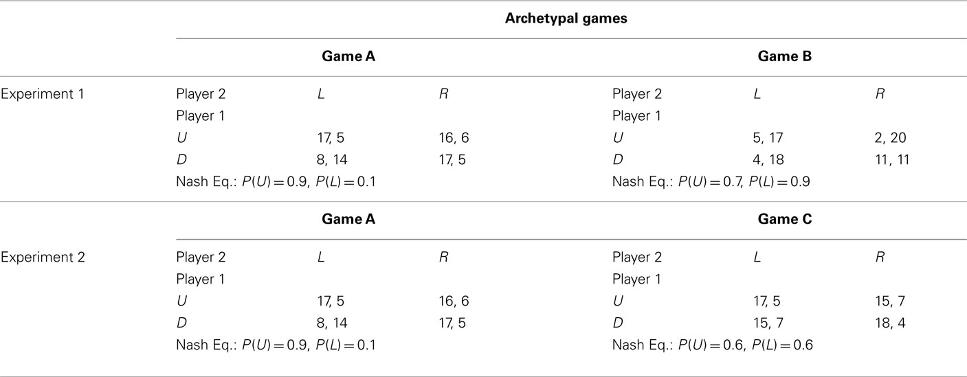
Table 1. The two pairs of completely mixed archetypal games used for building the game sequences in the two experiments.
Experiment 1
Four groups of subjects played four game sequences built starting from two 2 × 2 constant-sum games (henceforth game A and game B; see Table 1). Game A and B payoffs were chosen in such a way that equilibrium probabilities for one player were not so different [respectively, P(U) = 0.9 and 0.7], whereas the other player was supposed to reverse his/her strategy [respectively, P(L) = 0.1 and 0.9]. Moreover, to get a balanced experimental design, payoffs in each cell of the two games where chosen to sum up to the same constant.
To build each sequence, 60 “type A” games were obtained by multiplying game A’s payoffs for 60 randomly drawn constants2 (normally distributed with mean 10 and SD 4). The same procedure was used to obtain 60 “type B” games3. Type A and B games were then shuffled in such a way that in each block of 10 trials there were five type A and five type B games in random order. Thus, in each block of 10 trials subjects could face the same number of type A and type B games.
Participants
Thirty-two students from the faculties of Economics, Law, and Sociology of the University of Trento (Italy) participated in Experiment 1. Subjects were paid based on their cumulated payoff in 12 randomly selected trials plus a show-up fee (see Experimental Instructions in Appendix).
Results
Figure 1 reports the relative frequency of U and L choices in blocks of 10 trials, separately for type A and B games.
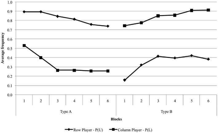
Figure 1. Observed proportions of U and L choices averaged over blocks of 10 trials, separately for type A and B games.
Observed behavior in type A games is not well approximated by Nash equilibrium. Row players play Nash mixture in the first two blocks [for which P(U) = 0.89], but the proportion of U choices eventually converges to 0.74. As for the column players, play starts close to random behavior in the first block and converges to 0.33, higher than the 0.1 predicted by Nash’s theory.
The predictive power of Nash equilibrium in type B games is also rather poor. In equilibrium, row players are supposed to choose action U with probability 0.7, whereas observed play converges to the relative frequency of 0.9. Column players are predicted to choose action L 90% of the times, but the observed proportion converges, from the third block, to about 0.4.
Experiment 2
Experiment 2 was identical to the previous one, except for the fact that games A and C were used to build the four sequences (see Table 1). Game C was chosen in such a way that equilibrium probabilities were, for both players, close to equal chance; thus, no reversal of choice strategies was implied. Also in this case, in each cell of games A and B, payoffs sum up to the same constant.
Participants
Thirty-two students from the faculties of Economics, Law, and Sociology of the University of Trento (Italy) participated in Experiment 2. Subjects were paid based on their cumulated payoff in 12 randomly selected trials plus a show-up fee (see Experimental Instructions in Appendix).
Results
Figure 2 illustrates the results from Experiment 2. The relative frequency of U choices in type A games is systematically higher than that predicted by Nash’s theory, similarly to what happened in Experiment 1. It is interesting to note that, in type C games, empirical behavior of both row and column players eventually converges to Nash play [P(U) = P(L) = 0.6], confirming that Nash equilibrium is a good predictor (at least in the long run) when predicted choice probabilities are close to 0.5 (Erev and Roth, 1998; Erev and Haruvy, in preparation).
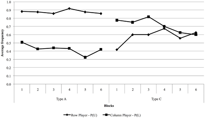
Figure 2. Observed proportions of U and L choices averaged over blocks of 10 trials, separately for type A and C games.
Cross-game Learning
The question of how play in type A games is affected by the simultaneous play of games of a different kind can be easily answered by comparing choice frequencies in type A games in the two experiments. To this end, we ran a two-way, repeated measures analysis (results are summarized in A1 and A2 in Appendix), in which we tested the effects of the variables Experiment (i.e., the experimental condition) and Time, and of their interaction on choice frequencies for both row and column players. As a result, the variable Experiment has no significant effect, implying that no cross-game learning is taking place. We conclude that, when games of just two types are present, subjects are able to recognize the two strategic situations and act without confounding them.
The Model
Since when McCulloch and Pitts (1943) introduced the first neuronal model in 1943, artificial neural networks have usually been intended as mathematical devices for solving problems of classification and statistical pattern recognition (see for example, Hertz et al., 1991; Bishop, 1995). For this reason, neural network-based learning models are the most natural candidates for predicting data from our multigame experiments, wherein a categorization task is implicit.
We present here a variant of the PB0 model proposed in Marchiori and Warglien (2008), which we call SOFTMAX-PB0. This model is a simple perceptron, i.e., a one-layer feed-forward neural network (Rosenblatt, 1958; Hopfield, 1987); its input units (labeled with ini) are as many as the game payoffs, whereas its output units (labeled with outj) are as many as the actions available to a player. Different from the PB0 model, according to SOFTMAX-PB0, the activation states of output units are determined via the softmax rule (1), and can thus be readily interpreted as choice probabilities.

The term wij in (1) is the weight of the connection from input unit ini to output unit outj.
Compared to the use of the tanh activation function, calculating activation states via the softmax rule avoids the premature saturation of output units, and in general results in a better fit of the data and has important theoretical implications4.
Adaptive learning from time step t − 1 to time step t occurs through modifications in the connection weights as follows:

with:

In the current model, the parameter λ that appears in (3) is replaced by a deterministic function, whose value at time step t is defined as the ratio between the experienced cumulated regret and the maximum cumulated regret. It is worth noting that the SOFTMAX-PB0 is non-parametric, as also in the softmax activation function (1) no free parameters are introduced.
In (3), targj is the ex-post best response to the other players’ actions, and it is equal to one if action j was the best response, and zero otherwise. Finally, the regret term is simply defined as the difference between the maximum obtainable payoff given other players’ actions and the payoff actually received.
The SOFTMAX-PB0 and the PB0 models, behavior is the result of adjustments in the direction of the ex-post best response (ex-post rationalizing process), and these adjustments are proportional to a measure of regret, consistently with findings in the neuroscientific field (Coricelli et al., 2005; Daw et al., 2006).
The SOFTMAX-PB0 model, as well as the PB0 one, presents some architectural analogies with established models of learning in games, but it has also some peculiar features that differentiate it from its competitors, as illustrated in Figure 3. Established learning models have two main cyclic component processes: (1) behavior is generated by some stochastic choice rule that maps propensities into probabilities of play; (2) Learning employs feedback to modify propensities, which in turn affect subsequent choices.
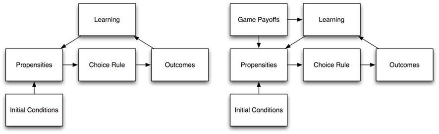
Figure 3. Adapted from Marchiori and Warglien (2008): General architecture of a “propensities and stochastic choice rule” learning model (left), and general architecture of the (SOFTMAX-)PB0 model (right).
The (SOFTMAX-)PB0 model’s architecture is only partially similar to that of the other learning models. What distinguishes our models is the direct dependence of choice behavior upon game payoffs (represented in the “input layer”). Whereas in a typical economic learning model choice is a function of propensities only, here it is function of both propensities and the payoffs of the game.
This architecture provides the (SOFTMAX-)PB0 model with a peculiar capability to discriminate among different games. Conventional learning models in economics are designed for repeated games. There is learning, but no discrimination or generalization: the simulated agent is unable to discriminate between different games at a certain moment; if given abruptly a different game, it would respond in the same way, or just throw away what it had previously learned. On the other hand, discrimination is something perceptrons do very well, and since the output is also directly affected by perceived inputs (the activation states of input units), a network, besides learning, will respond differently to different games.
The Sampling Paradigm for Modeling Learning
Particularly relevant to the current analysis are the two contribution by Erev (2011) and by Gonzalez and Dutt (2011), in which the INERTIA SAMPLING AND WEIGHTING (I-SAW) and INSTANCE BASED LEARNING (IBL) models are proposed. According to these models, agents are supposed to make their decisions based on samples from their past experience. These models have been shown to capture important regularities of human behavior in decisions from experience (Erev et al., 2010; Gonzalez et al., 2011).
The most obvious way of modifying these models in order to perform conditional behavior is that of considering agents that draw from a subset of past experiences that are relevant to the current decision task. However, such an implementation would imply an exogenous intervention for the classification of the situation at hand, requiring an explicit theory of what is similar/relevant to what. On the other hand, the modeling approach based on sampling easily gives account for learning spillover effects (Marchiori et al., unpublished).
However, the classification operated by the (SOFTMAX-)PB0 model is endogenous; agents just observe inputs and respond to them without any external intervention and the entire process of classification is implicit in the structure of the model itself.
Materials and Methods
Predicted choice frequencies were obtained by averaging results over 150 simulations, and, for parametric models, this procedure was repeated for each parameter configuration. Table 2 collects the description of the portions of the parameter spaces investigated.

Table 2. Explored portions of parameter spaces and the parameter configurations yielding the lowest average MSD in the two experiments.
We tested models’ predictive power by considering estimated choice frequencies corresponding to the parameter configurations that minimized the mean square deviation (henceforth MSD; Friedman, 1983; Selten, 1998) in our two experiments. Considering average MSD scores in the two experiments does not penalize directly the number of free parameters of a model; therefore, in this analysis, parametric models are advantaged over the non-parametric PB0 and SOFTMAX-PB0 ones.
In our comparative analysis, we considered the following learning models: normalized fictitious play (NFP; Erev et al., 2007); normalized reinforcement learning (NRL; Erev et al., 2007); Erev and Roth’s reinforcement learning (REL; Erev and Roth, 1998); reinforcement learning (RL; Erev et al., 2007); stochastic fictitious play (Erev et al., 2007); and self-tuning experience weighted attraction (stEWA; Ho et al., 2007). Section “Competitor Models and Investigated Portions of Parameter Spaces” in Appendix briefly reviews these models.
Simulation Results and Discussion
Although simple perceptrons suffer severe theoretical limitations in the discrimination tasks they can carry out (Minsky and Papert, 1969; Hertz et al., 1991), our simulation results show that they are nonetheless able to discriminate between two different strategic situations and predict well choice behavior observed in our multigame experiments. Simulation results are collected in Figure 4 and, more in detail, in Tables 3 and 4.
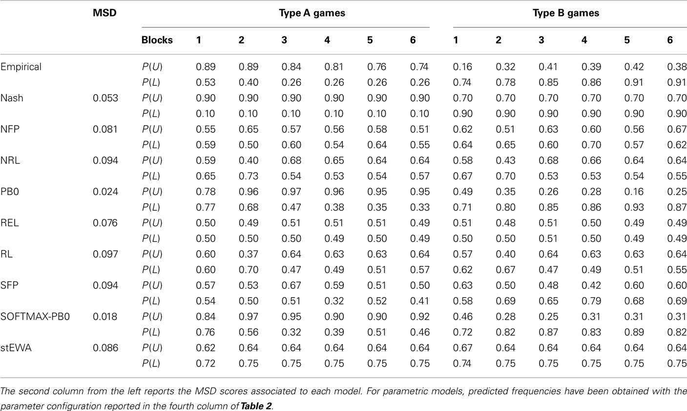
Table 3. Predicted and observed choice frequencies in Experiment 1.
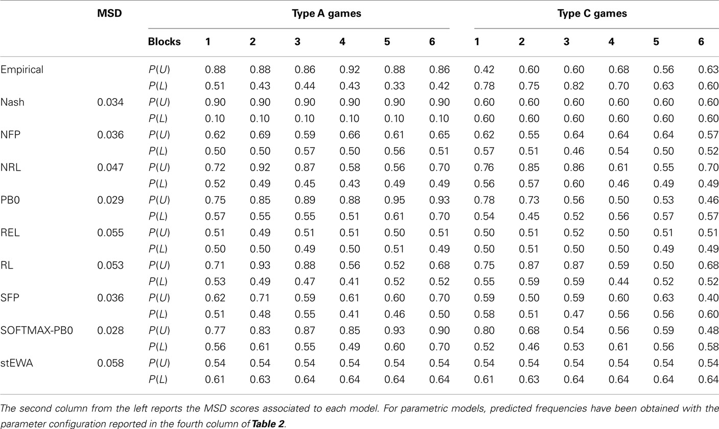
Table 4. Predicted and observed choice frequencies in Experiment 2.
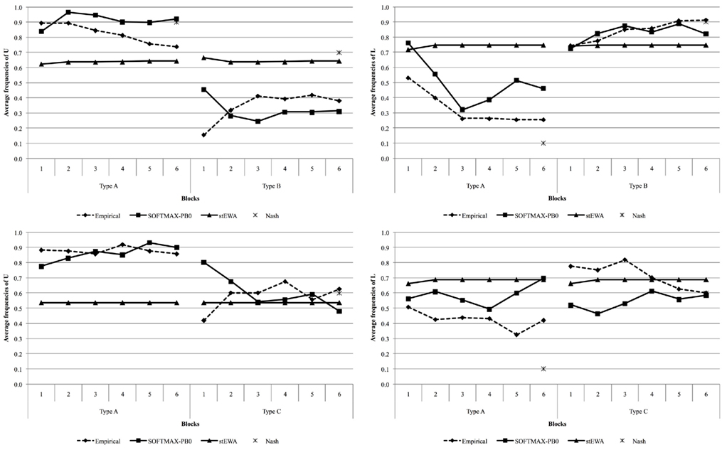
Figure 4. Predicted and observed choice frequencies in Experiment 1 (top panels) and 2 (lower panels).
Established learning models are not able to discriminate between the two different game structures, providing the same “average” behavior for both types of games (see Tables 3 and 4), and are always outperformed by Nash equilibrium. On the contrary, the SOFTMAX-PB0 and PB0 models are able to replicate subjects’ conditional behavior, due to the direct dependence of their response on game payoffs, remarkably outperforming Nash equilibrium and all the other models of learning considered in this analysis.
Comparison of the performance of the PB0 and SOFTMAX-PB0 models shows how the introduction of the softmax rule for calculating output units’ activations improves the fit of the data.
Cross-Game Learning
As reported at the end of Section “The Multigame Experiments,” our experimental data do not provide evidence of cross-game learning. In regard to this, simulation results show that there is a partial qualitative parallelism between the (SOFTMAX-)PB0 model’s predictions and observed behavior. For example, for the row player, the (SOFTMAX-)PB0 model provides very similar trajectories in the two experiments. However, if we consider column player’s predicted behavior, the (SOFTMAX-)PB0 model produces very different trajectories in the two experiments. This might imply that the (SOFTMAX-)PB0’s structure is not complex enough to completely avoid spillover effects across games, although this aspect would deserve a more systematic investigation. However, it is not difficult to imagine situations in which learning spillovers do take place and this feature of the (SOFTMAX-)PB0 model would turn out to be advantageous.
Conclusion
The present paper presents an experimental design in which subjects faced a sequence of different interactive decision problems, making a step forward in the realism of the situations simulated in the lab. The problems in the sequences were different instances of two 2 × 2 completely mixed games. Thus, at each trial, subjects’ task was twofold: recognize the type of the current decision problem, and then act according to this categorization. Our experimental results show that subjects are able to recognize the two different game structures in each sequence and play accordingly to this classification. Moreover, our experimental data do not provide evidence of cross-game learning, as there are no significant differences in the play of type A games in the two experiments.
Our experiments were designed with the precise goal of testing the discrimination capability of the PB0 and SOFTMAX-PB0 neural network models in comparison with that of other established models of learning proposed in the Psychology and Economics literature. Simulation results show that traditional “attraction and stochastic choice rule” learning models are not able to discriminate between the different strategic situations, providing a poor “average” behavior, and are always outperformed by Nash equilibrium. On the contrary, the (SOFTMAX-)PB0 model is able to replicate subjects’ conditional behavior, due to the direct dependence of its response on game payoffs, and performs better than standard theory of equilibrium. This latter fact is particularly remarkable; in our experiments, the two classes of games were built based on their Nash equilibrium, so that the classification was induced by the different equilibrium predictions. On the contrary, our neural network models of adaptive learning were able to classify the different game structures without any external and predetermined partition of the game space.
We are well aware of the need for a more systematic and comprehensive analysis of categorization in games. Further experimental research could focus, for example, on sequences with more than two types of games, or on the effects of different degrees of payoff perturbations on learning spillovers.
Conflict of Interest Statement
The authors declare that the research was conducted in the absence of any commercial or financial relationships that could be construed as a potential conflict of interest.
Acknowledgments
We are grateful to Luigi Mittone, director of the CEEL experimental laboratory (University of Trento, Italy) where our experiments were conducted. Also the support of Marco Tecilla and of the CEEL staff is gratefully acknowledged. This project was supported by the Fondazione Università Ca’ Foscari and a fellowship from the Lady Davis Foundation.
Footnotes
- ^Games with a unique Nash equilibrium in mixed strategies.
- ^Only positive values were considered.
- ^Thus type A and B games had, respectively, the same mixed strategy equilibrium of games A and B.
- ^Moreover, when outputs are calculated via (1), the updating rule (3) leads to Cross-Entropy minimization or, in other terms, to the maximization of the likelihood of observing a given training set.
References
Camerer, C. F., and Ho, T.-H. (1999). Experience-weighted attraction learning in normal form games. Econometrica 67, 837–874.
Cooper, D. J., and Kagel, J. H. (2003). Lessons learned: generalizing learning across games. Am. Econ. Rev. 93, 202–207.
Cooper, D. J., and Kagel, J. H. (2008). Learning and transfer in signaling games. Econ. Theory 34, 415–439.
Coricelli, G., Critchley, H. D., Joffily, M., O’Doherty, J. P., Sirigu, A., and Dolan, R. J. (2005). Regret and its avoidance: a neuroimaging study of choice behavior. Nat. Neurosci. 8, 1255–1262.
Daw, N. D., O’Doherty, J. P., Dayan, P., Seymour, B., and Dolan, R. J. (2006). Cortical substrates for exploratory decisions in humans. Nature 441, 876–879.
Devetag, G. (2005). Precedent transfer in coordination games: an experiment. Econ. Lett. 89, 227–232.
Erev, I. (2011). On surprise, change, and the effect of recent outcomes. Front. Cogn. Sci. [Paper pending published].
Erev, I., Bereby-Meyer, Y., and Roth, A. E. (1999). The effect of adding a constant to all payoffs: experimental investigation, and implications for reinforcement learning models. J. Econ. Behav. Organ. 39, 111–128.
Erev, I., Ert, E., Roth, A. E., Haruvy, H., Herzog, S. M., Hau, R., Hertwig, R., Stewart, T., West, R., and Lebiere, C. (2010). A choice prediction competition: choices from experience and from description. J. Behav. Decis. Mak. 23, 15–47.
Erev, I., and Roth, A. E. (1998). Predicting how people play games: reinforcement learning in experimental games with unique, mixed-strategy equilibria. Am. Econ. Rev. 88, 848–881.
Erev, I., Roth, A. E., Slonim, R. L., and Barron, G. (2002). Predictive value and the usefulness of game theoretic models. Int. J. Forecast. 183, 359–368.
Erev, I., Roth, A. E., Slonim, R. L., and Barron, G. (2007). Learning and equilibrium as useful approximations: accuracy of prediction on randomly selected constant sum games. Econ. Theory 33, 29–51.
Ert, E., and Erev, I. (2007). Replicated alternatives and the role of confusion, chasing, and regret in decisions from experience. J. Behav. Decis. Mak. 20, 305–322.
Gonzalez, C., and Dutt, V. (2011). Instance-based learning: integrating sampling and repeated decisions from experience. Psychol. Rev. 118, 523–551.
Gonzalez, C., Dutt, V., and Lejarraga, T. (2011). A loser can be a winner: comparison of two instance-based learning models in a market entry competition. Games 2, 136–162.
Hertz, J. A., Krogh, A. S., and Palmer, R. G. (1991). Introduction to the Theory of Neural Computation. Redwood City, CA: Addison-Wesley Publishing Company.
Ho, T.-H., Camerer, C. F., and Chong, J.-K. (2007). Self-tuning experience-weighted attraction learning in games. J. Econ. Theory 133, 177–198.
Hopfield, J. J. (1987). Learning algorithms and probability distributions in feed-forward and feed-back networks. Proc. Natl. Acad. Sci. U.S.A. 84, 8429–8433.
Kagel, J. H. (1995). Cross-game learning: experimental evidence from first-price and English common value auctions. Econ. Lett. 49, 163–170.
Knez, M., and Camerer, C. F. (2000). Increasing cooperation in prisoner’s dilemmas by establishing a precedent of efficiency in coordination games. Organ. Behav. Hum. Decis. Process. 82, 194–216.
Marchiori, D., and Warglien, M. (2008). Predicting human behavior by regret-driven neural networks. Science 319, 1111–1113.
McCulloch, W. S., and Pitts, W. H. (1943). A logical calculus of the ideas immanent in nervous activity. Bull. Math. Biophys. 5, 115–133.
Rankin, F. W., Van Huyck, J. B., and Battalio, R. C. (2000). Strategic similarity and emergent conventions: evidence from similar stag hunt games. Games Econ. Behav. 32, 315–337.
Rosenblatt, F. (1958). The perceptron: a probabilistic model for information storage and organization in the brain. Psychol. Rev. 65, 386–408.
Sgroi, D., and Zizzo, D. J. (2007). Neural networks and bounded rationality. Physica A 375, 717–725.
Sgroi, D., and Zizzo, D. J. (2009). Learning to play 3 × 3 games: neural networks as bounded rational players. J. Econ. Behav. Organ. 69, 27–38.
Appendix
Experimental Instructions
Instructions
You are participating in an experiment on interactive decision-making funded by the Italian Ministry of University and Research (MIUR). This experiment is not aimed at evaluating you neither academically nor personally, and the results will be published under strict anonymity.
You will be paid based on your performance, privately and in cash, according to the rules described below.
During the experiment, you will not be allowed to communicate with the other participants, neither verbally nor in any other way. If you have any problem or questions, raise your hand and a member of the staff will immediately contact you.
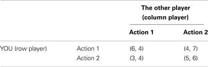
The experiment will consist of 120 rounds, and at each round you will face an interactive decision task. Specifically, at each round, you will be randomly matched with another participant and your payoff will depend on both your decision and that of the other participant. The structure of each decision task will be represented as shown in the following figure:
You have been assigned the role of “row player”: therefore, the other player will always play the role of “column player.”
For each player two actions are available (labeled “Action 1” and “Action 2”). For every possible combination of actions by row and column players, there corresponds a cell in the matrix. In every cell there are two numbers between parentheses: the first number corresponds to YOUR payoff (in experimental currency units), and the second corresponds to the payoff of the other player (again in experimental currency units).
As an example, referring to the matrix reported below, if YOU choose to play “Action 1” and the other player chooses to play “Action 2,” then the payoffs will be four for YOU (row player) and seven for the other player (column player).
Please, remember that the experiment will consist of 120 rounds. At each round, you will be shown a sequence of two screenshots.
The first screenshot will show you the current payoff matrix, and you will be invited to make a decision. In order to make a decision, you must type either “1” or “2” in the box labeled “your decision,” and then click on the button “confirm.” Once you have clicked the confirmation button, you cannot change your decision. You will have a maximum of 30 s to choose: after those 30 s a blinking red message will appear on the right-up corner of the screen and spur you to make a decision. Delaying your decision will cause the other participants to wait for you.
Once all players have made their decision, the second screenshot will appear on your monitor. In this second screenshot there will be reported the action you chose, the action chosen by the other player, your respective payoffs, and the payoff matrix you saw in the first screenshot.
The second screenshot will be visible on your monitor for 10 s and then another round will start.
This process will be repeated for 120 times. After all rounds have been played, the experiment will be over and the procedure of payment will start. In order to determine your payment, 12 integers between 1 and 120 will be randomly drawn without replacement. In this way, 12 out of the 120 rounds will be randomly selected and you will be paid based on their outcomes. One experimental currency unit is equivalent to 10 eurocents (10 experimental units = 1 euro). Moreover, independently from your performance, you will be paid an additional show-up fee of 5 euro.
Before the beginning of the experiment, you will be asked to fill a questionnaire to verify whether the instructions have been understood. Then the experiment will start.
At the end of the experiment, you will be asked to fill a questionnaire for your payment.
Thank you for your kind cooperation!
Repeated Measures ANOVA
Competitor Models and Investigated Portions of Parameter Spaces
The REL model (Erev et al., 1999, 2002)
Attractions updating. The propensity of player i to play her k-th pure strategy at period t + 1 is given by:

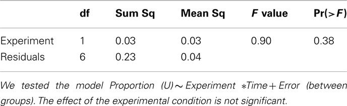
Table A1. Two-way, repeated measures ANOVA (row players).
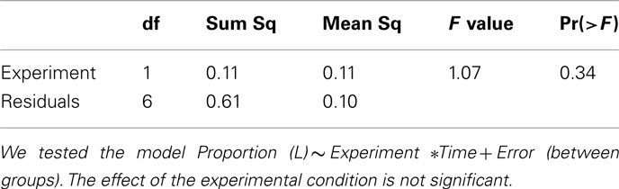
Table A2. Two-way, repeated measures ANOVA (Column players).
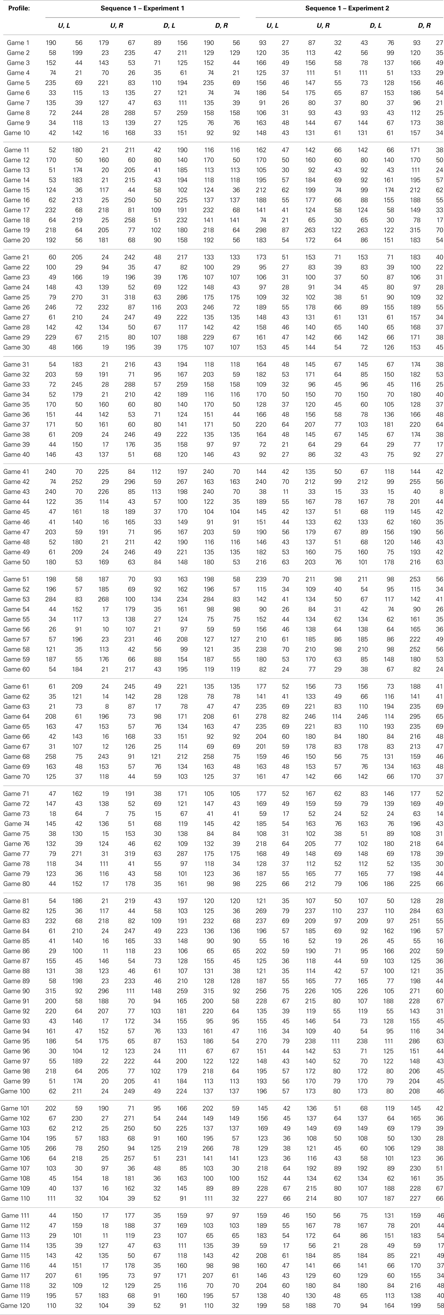
Table A3. Two of the game sequences played in Experiment 1 and 2.
where Cij(t) indicates the number of times that strategy j has been chosen in the first t rounds, x is the obtained payoff, and N(1) a parameter of the model determining the weight of the initial attractions.
Stochastic choice rule. Player i’s choice probabilities are calculated as follows:
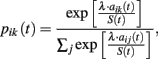
where λ is a sensitivity parameter, whereas S(t) gives a measure of payoff variability.
Initial attractions. S(1) is defined as the expected absolute distance between the payoff from random choices and the expected payoff given random choices, denoted as A(1). At period t > 1:

where x is the received payoff, m the number of player i’s pure strategies, and A(t + 1) is:

Initial attractions are such that aij(1) = A(1), for all i and j. This model has two free parameters, namely λ and N(1).
The RL model (Erev and Roth, 1998; Erev et al., 2007)
Initial propensities. Initial propensities are set equal to the expected payoff from random choice [denoted by A(1)], so that aij(1) = A(1), for all i and j.
Attractions updating. Propensities are updated as follows:

where vij(t) is the realized payoff, and w parameter expressing the weight of past experience. The updating rule above implies agents’ insensitivity to foregone payoffs.
Stochastic choice rule. Choice probabilities are calculated as follows:
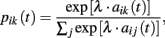
where λ is a payoff sensitivity parameter.
The NRL model (Erev et al., 2007)
Initial propensities. Initial propensities are set equal to the expected payoff from random choice [denoted by A(1)], so that aij(1) = A(1), for all i and j.
Attractions updating. Propensities are updated according to the following:

where vij(t) is the realized payoff and w a weight parameter. The updating rule implies agents’ insensitivity to foregone payoffs.
Stochastic choice rule. Choice probabilities are defined as:
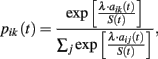
where S(t) gives a measure of payoff variability and λ is payoff sensitivity parameter.

where recenti is the most recent experienced payoff from action i = 1, 2. At the first period, recenti = A(1), and S(1) is set equal to λ. Similarly to the NFP model, payoff sensitivity [the ratio λ/S(t)] is assumed to decrease with payoff variability.
The NFP model (Erev et al., 2007; Ert and Erev, 2007)
Initial propensities. Initial propensities are set equal to the expected payoff from random choice [denoted by A(1)], so that aij(1) = A(1), for all i and j.
Attractions updating. Propensities are updated according to the following:
aij(t + 1) = (1 − w)·aij(t) + w·vij(t), for all i and j,
where vij(t) is the expected payoff in the selected cell and w is a parameter that measures sensitivity to foregone payoffs.
Stochastic choice rule. Choice probabilities are obtained as follows:
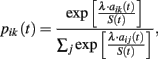
where S(t) gives a measure of payoff variability, and λ is payoff sensitivity parameter.

where recenti is the last experienced payoff from action i = 1, 2. At the first period, recenti = A(1), and S(1) is set equal to λ.
The SFP model (Erev et al., 2007)
Initial propensities. Initial propensities are set equal to the expected payoff from random choice [denoted by A(1)], so that aij(1) = A(1), for all i and j.
Attractions updating. Propensities are updated according to the following:
aij(t + 1) = (1 − w)·aij(t) + w·vij(t), for all i and j,
where vij(t) is the expected payoff in the selected cell and, w is a parameter that measures sensitivity to foregone payoffs.
Stochastic choice rule. Choice probabilities are calculated as follows:
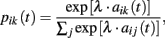
where λ is a payoff sensitivity parameter.
The stEWA model (Camerer and Ho, 1999; Ho et al., 2007)
Attractions updating. At time t, player i associates to his j-th pure strategy the attraction aij(t), given by:

where si(t) and s −i(t) are the strategies played by player i and his opponents, respectively, and πi(sij,s −i(t)) is the ex-post payoff deriving from playing strategy j, and I(·) is the Kronecker function. Functions δij(t) and Φi(t) are called, respectively, attention function and change detector function. The latter depends primarily on the difference between the relative frequencies of chosen strategies in the most recent periods and the relative frequencies calculated on the entire series of actions. The attention function essentially determines the importance that players give to past experience.
Stochastic choice rule. Choice probabilities are calculated as follows:

where λ is the unique free parameter of the model.
Initial attractions. Authors suggest at least four ways of setting initial attractions aij(0). In our implementation, initial attractions are set equal to the average payoff from random choice, leading to first period uniformly distributed choices.
Keywords: neural networks, learning, categorization, regret, cross-game learning, mixed strategy equilibrium, repeated games
Citation: Marchiori D and Warglien M (2011) Neural network models of learning and categorization in multigame experiments. Front. Neurosci. 5:139. doi: 10.3389/fnins.2011.00139
Received: 15 November 2011; Accepted: 04 December 2011;
Published online: 27 December 2011.
Edited by:
Eldad Yechiam, Technion Israel Institute of Technology, IsraelReviewed by:
Eldad Yechiam, Technion Israel Institute of Technology, IsraelItzhak Aharon, The Interdisciplinary Center, Israel
Cleotilde Gonzalez, Carnegie Mellon University, USA
Copyright: © 2011 Marchiori and Warglien. This is an open-access article distributed under the terms of the Creative Commons Attribution Non Commercial License, which permits non-commercial use, distribution, and reproduction in other forums, provided the original authors and source are credited.
*Correspondence: Davide Marchiori, Department of Economics, National Chengchi University, Tz-nan Road 64, Section 2 Wenshan, Taipei 116, Taiwan. e-mail:ZGF2aWRlQG5jY3UuZWR1LnR3