


- 1 Department of Experimental Psychology, University of Oxford, Oxford, UK
- 2 Department of Psychology, Center for Mind, Brain and Computation, Stanford University, Stanford, CA, USA
- 3 School of Psychology and Sagol School of Neuroscience, Tel-Aviv University, Tel-Aviv, Israel
When people make decisions, do they give equal weight to evidence arriving at different times? A recent study (Kiani et al., 2008) using brief motion pulses (superimposed on a random moving dot display) reported a primacy effect: pulses presented early in a motion observation period had a stronger impact than pulses presented later. This observation was interpreted as supporting the bounded diffusion (BD) model and ruling out models in which evidence accumulation is subject to leakage or decay of early-arriving information. We use motion pulses and other manipulations of the timing of the perceptual evidence in new experiments and simulations that support the leaky competing accumulator (LCA) model as an alternative to the BD model. While the LCA does include leakage, we show that it can exhibit primacy as a result of competition between alternatives (implemented via mutual inhibition), when the inhibition is strong relative to the leak. Our experiments replicate the primacy effect when participants must be prepared to respond quickly at the end of a motion observation period. With less time pressure, however, the primacy effect is much weaker. For 2 (out of 10) participants, a primacy bias observed in trials where the motion observation period is short becomes weaker or reverses (becoming a recency effect) as the observation period lengthens. Our simulation studies show that primacy is equally consistent with the LCA or with BD. The transition from primacy-to-recency can also be captured by the LCA but not by BD. Individual differences and relations between the LCA and other models are discussed.
Introduction
The process of decision making has been the subject of intensive recent investigations in both experimental psychology (Usher and McClelland, 2001; Ratcliff and Smith, 2004; Brown and Heathcote, 2005; Bogacz et al., 2006; Ratcliff and McKoon, 2008; van Ravenzwaaij et al., 2012) and neuroscience (Huk and Shadlen, 2005; Gold and Shadlen, 2007; Ratcliff et al., 2007; Wong et al., 2007; Wang, 2008; Ditterich, 2010; Rorie et al., 2010). A central idea emerging from these investigations is that decision makers take multiple samples of noisy evidence and integrate them over time until the integrated evidence reaches a decision boundary. The time to reach the bound determines the reaction time (Gold and Shadlen, 2001, 2002; Roitman and Shadlen, 2002). Some of these decision making models generate optimal decisions in the sense that they achieve the shortest possible mean reaction time for a fixed error-rate (Wald, 1946; Gold and Shadlen, 2001, 2002; Bogacz et al., 2006). In addition, neurophysiological studies have reported that when monkeys make decisions about the direction of motion in a noisy moving dots display, neurons in several visual-motor integration areas (e.g., the lateral intraparietal cortex, LIP) show ramping activity consistent with the integration of evidence (Hanes and Schall, 1996; Gold and Shadlen, 2000, 2001; Horwitz and Newsome, 2001; Shadlen and Newsome, 2001).
A number of computational models that can account for both the behavioral and physiological choice data have been developed. These models not only account for the accuracy of participants’ responses, but also for details of the distributions of response times and their dependence on experiment conditions such as difficulty levels and speed-accuracy instructions (Ratcliff and McKoon, 2008).
The starting point for a wide range of decision making research is the drift-diffusion model (Ratcliff, 1978; Ratcliff and Rouder, 1998; Ratcliff and McKoon, 2008). In this model, the difference in evidence supporting each of two decision-alternatives is accumulated linearly over time, without loss or distortion. Here we consider a variant of this model that is often used to address neurophysiological data (Mazurek et al., 2003; Figure 1B). This model is represented as a process in which accumulators integrate the difference in the momentary evidence for the two alternatives via a combination of feed-forward excitation and inhibition, such that positive evidence for one alternative is negative evidence for the other.
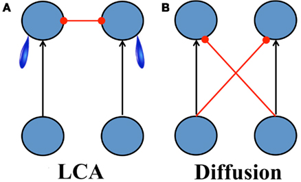
Figure 1. Architecture of the two-choice reaction-time models. (A) The leaky competing accumulator model (Usher and McClelland, 2001), (B) Mazurek et al. (2003) model. Arrows and filled circles indicate excitatory and inhibitory connections respectively. Blue tears indicate leakage.
In recent years, several researchers have proposed decision making models that do not adhere to the perfect integration of the drift-diffusion model. These models include variations based on the Decision Field Theory (Busemeyer and Townsend, 1993; Roe et al., 2001; Johnson and Busemeyer, 2005), the neurophysiologically grounded attractor network model (Wang, 2002; Wong and Wang, 2006) and the leaky competing accumulator model (LCA; Usher and McClelland, 2001; Bogacz et al., 2007). To varying degrees, all of these models draw on inspiration from principles of neural computation and attempt to capture ways in which decision making deviates from perfect optimality. For example, these models incorporate the possibility of leakage or decay of information, as well as mutual inhibition between the representations of the decision-alternatives, and both the attractor and LCA models incorporate non-linearities that can affect information integration.
In the present work we focus primarily on the LCA (Figure 1A). In this model, as in the model of Mazurek et al. (2003), accumulators representing the available alternatives accumulate noisy evidence over time, but in this case, there is no feed-forward inhibition. Instead, accumulated evidence is subject to leak, and the accumulators compete with each other through mutual inhibition. The LCA has been successful in capturing a number of features of human decision making data (Usher and McClelland, 2001, 2004; Bogacz et al., 2007; Gao et al., 2011; Tsetsos et al., 2011). This model is intermediate in complexity between the other models; it introduces a lower bound on activation, unlike the decision field theory, but it lacks additional features that are present in the attractor model, including an activity dependent gating of special channels that change its leakage characteristics. We retain the lower bound at 0 because it has important implications for aspects of the dynamics of decision making that have already received support in another recent study (Tsetsos et al., 2011). As we shall see, this lower bound will also play a role in understanding the findings we will present in the present article. The greater simplicity of the LCA compared to the attractor model (Wang, 2002) makes it more tractable for analysis, and this is one of the prime reasons for our focus on the LCA. We are open, however, to the possibility that the added features of the attractor model may be important, and we will return to this class of models in the Section “Discussion.”
Research on decision making often employs what is called the free-response paradigm, which sets up decision-time under the control of the observer. In this paradigm, a stimulus is presented on each trial, and participants are assumed to integrate evidence until they reach a decision bound. All of the models under consideration assume that this bound represents a criterion amount of accumulated evidence. However, the models differ in their handling of decision making in time-controlled paradigms, in which evidence is presented for a period of time controlled by the experimenter, and in which the overt response is prompted by a cue called a go cue. When difficult stimuli are used in such experiments, stimulus sensitivity (measured by d′) is 0 with very short evidence accumulation times, then rises to a finite asymptotic level after about 1 s, remaining constant even if more integration time is allowed (Wickelgren, 1977; Usher and McClelland, 2001; Kiani et al., 2008). The LCA and the diffusion model have different ways of addressing this finding. In the LCA and related models, evidence accumulation is assumed to continue until the end of the evidence evaluation period, at which point the decision maker is thought to choose the alternative associated with the most active accumulator. The fact that accuracy levels off is attributed to an imbalance between leak and inhibition, as discussed in more detail below. In contrast, in the Mazurek et al. version of the drift-diffusion model, decision sensitivity can increase without bound as integration time increases, since there is no loss or distortion in evidence accumulation; the model predicts that the signal to noise ratio should increase with To address the fact that performance levels off in time-controlled paradigms, Mazurek et al. (2003) proposed that, just as in free-response paradigms, participants employ a decision bound in time-controlled situations, such that evidence integration stops when the boundary is reached, even though stimulus input continues and the response must be withheld until a cue to respond is presented (see also Ratcliff, 2006). Because of the presence of this decision bound, even in time-controlled situations, we call this model the bounded diffusion (BD) model in the remainder of this article.
In a recent paper (Kiani et al., 2008), the authors proposed a way to determine whether the leveling off of accuracy in time-controlled paradigms is more consistent with the presence of a bound, or alternatively with leaky integration. The paper considered the BD model and what they referred to as the leaky accumulation model, a variant of the LCA in which leakage is stronger than inhibition (henceforth called the leak-dominant LCA). The leaky accumulation model predicts that late information is more important (a pattern called recency) since early information has more time to leak away. This contrasts with the BD model, which predicts that early information is more important (a pattern called primacy) because late information is more likely to arrive after the bound is reached and therefore to be ignored.
Two pieces of evidence were shown to support the primacy pattern in the experiment. The first was based on the reverse correlation technique. The reverse correlation analysis is applied to experimental trials in which the evidence (in the form of dot motion) is completely random. Trials are grouped according to the observed response choice between the two available alternatives, which we will label A and B. The analysis examines the averaged input signal in the time course of the entire trial in the two groups. If the analysis reveals no difference between the A and B groups at some time points, it means that inputs at those time points do not contribute to the outcome. On the other hand, if the analysis reveals a large difference between the two groups of trials at some time points, it means inputs at those time points are contributing to determining the response. When this analysis was applied to model simulations, it confirmed that the BD model predicts a primacy pattern while the leaky accumulation model predicts a recency pattern (Figure 2A). The same analysis based on behavioral data demonstrated a primacy pattern (Figure 2B). The second source of support for the primacy pattern was based on a pulse perturbation study, using 200 ms motion pulses that influenced monkey’s choices in the direction of the pulse. The size of the pulse effect was largest when the pulse was applied early in the trial, and decreased when pulses occurred later, consistent with BD rather than leaky accumulation.
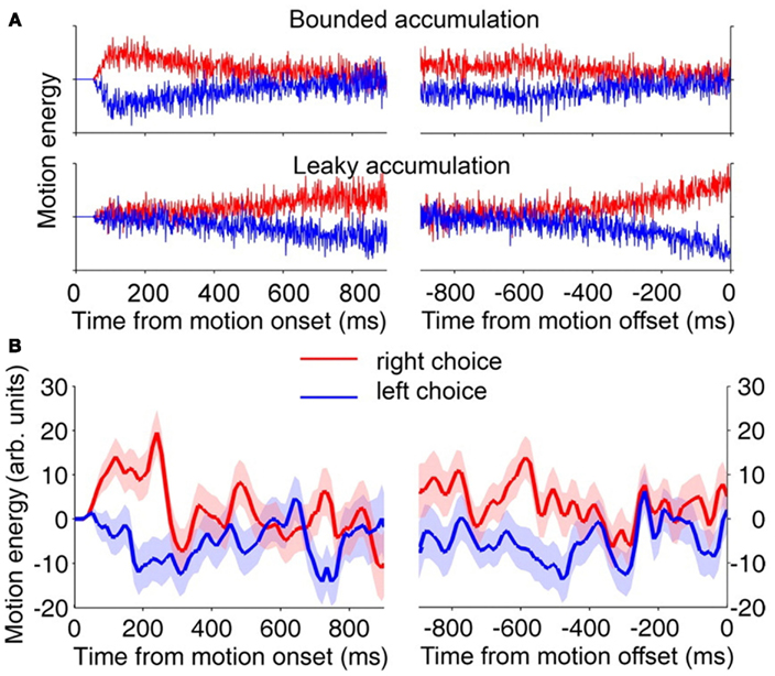
Figure 2. Reverse correlation analysis (reproduced from Kiani et al., 2008). (A) Expected separation of motion energy profiles for rightward (red) and leftward (blue) choices for bounded diffusion (top) and leak-dominant LCA (bottom). Late information is more critical in the leak-dominant LCA model while early information is more critical in the bounded diffusion model. (B) Left, signals aligned with motion onset, right signals aligned with motion offset. One can observe that in the data (Panel B), the difference between the evidence that favors the response (red) and the one that opposes it (blue) is larger at the beginning of the choice interval.
In the present paper, we further examine the temporal weighting of evidence in experiments and in the LCA and BD models. Our examination is motivated by both empirical and model-based observations presented in Usher and McClelland (2001). On the empirical side, the result of the perturbation study in Kiani et al. (2008) stands in contrast with experimental findings reported in Usher and McClelland, 2001; Experiment 3). In that experiment, participants viewed a stream of interleaved S’s and H’s and reported after the end of the sequence which letter was predominant. While most of the trials contained sequences with a majority of either S or H, some of the trials contained equal numbers of S’s and H’s. Within the latter type of trials, one of the letters sometimes predominated early in the trial, with the other letter predominating later. Out of the six subjects, two showed a primacy bias, favoring the letter that predominated early in the sequence; two showed a recency bias, favoring the latter that predominated late; and two showed approximate balance, or little bias in either direction.
On the theoretical side, the LCA was able to account for all three types of behavior. While the model shows a recency pattern when leak is stronger than inhibition, it shows a primacy pattern when inhibition is stronger than leak, and it shows equal weight of early and late information when the strength of leak and inhibition are equal. All else being equal, balanced leak, and inhibition lead to greater accuracy, and indeed, the experimental data indicated the expected relationship between accuracy on trials when the number of S’s and H’s were different, and the degree of bias (either toward primacy or recency) exhibited on trials when the number of S’s and H’s was the same. Specifically, greater imbalance when the number of S’s and H’s was the same was associated with lower accuracy when the number of S’s and H’s was different.
The present study seeks to examine these empirical and model-based considerations further. On the empirical side, there are many differences between the experiments of Usher and McClelland (2001) and Kiani et al. (2008). Among other things, Usher and McClelland’s study involved six relatively unpracticed human participants who were not placed under strong time pressure. Kiani et al. used two highly practiced rhesus macaque monkey participants who received a go cue (on half of their experimental trials) coincident with the end of the stimulus presentation period, requiring them to respond within 500 ms. Several questions naturally arise: Would different patterns have been observed in the Kiani et al. study if it had been conducted on humans? Would individual differences have emerged had a larger number of participants been tested? Does extensive practice, or the need to be prepared to respond quickly, alter the tendency to observe a pattern of primacy vs. recency? The present research attempts to address these issues by using a paradigm quite similar to that of Kiani et al. (2008), employing highly practiced human participants, and manipulating the time pressure to respond across experiments. While our studies still use relatively small numbers of participants, we will see that there are indeed considerable individual differences within the set of participants.
Another goal of our research is to further explore the primacy pattern seen in some participants in both the Usher and McClelland (2001) and Kiani et al. (2008) studies. We will examine whether the LCA can capture the primacy pattern as well as the BD model does, and whether it can also capture other aspects of performance that are challenging to the BD model. As we will see, the LCA can exhibit primacy on some trials and recency on others, using the same parameter values. That is, it can exhibit a primacy effect when the length of the evidence accumulation interval is short, while exhibiting a recency effect when the length of the evidence accumulation interval is long. Our study will allow us to examine whether such a pattern can be observed in human participants.
We begin by reviewing an analysis of the LCA presented in Usher and McClelland (2001), extending this analysis by further examining the model using the same reverse correlation analysis as in Kiani et al. We then discuss the primacy-to-recency shift that can occur in the LCA model under certain ranges of its parameter values. Following this, we report two experimental studies with human observers1. In the first we place participants under high time pressure, using procedures similar to Kiani et al. and we find similar primacy patterns. In the second, we relax the time pressure by lengthening the response window and introducing longer trials, and we find the primacy bias diminishes significantly. We see individual differences in both studies, with one participant in the second study showing recency for short evidence integration periods and primacy for long integration periods. As the moving dots paradigm is a central one to the neuroscience of decision making (Burr and Santoro, 2001; Shadlen and Newsome, 2001; Kiani et al., 2008), we use moving dot stimuli in our study. Our use of temporally manipulated stimuli builds on the pioneering efforts of Huk and Shadlen (2005) and Wong et al. (2007) as well as the study of Kiani et al. (2008).
Materials and Methods
Experimental Methods
Moving dot stimuli
The moving dot stimuli were created following the method described in Kiani et al. (2008). The motion stimulus consisted of circular dots of radius 2 pixels, moving horizontally at a speed of 5°/s. Total dot density was 16.7 dots per degree squared per second. The stimulus was viewed through a circular aperture of radius 5°. The coherence of the motion stimulus varied from trial to trial and within trials as specified below.
Dots were randomly divided into three sets. One set of dots was displayed per frame, which lasted 13.33 ms. Each set of dots appeared on the monitor once every frame-triple, each of which contains three frames, spanning 50 ms. On every displayed frame, each dot had a (1 – coherence) probability of being redrawn at random coordinates within the circular aperture. Those not redrawn at random would be redrawn to move horizontally 5°/s in the direction specified for the trial. At 0% coherence, every dot would be redrawn randomly on every frame.
Experiment 1A
In this experiment, 80% of trials with duration 300 ms or greater contained a “pulse,” or momentary change of coherence level. A pulse consisted of a ±3.2% change in coherence level for 200 ms, or four frame-triples. The motion pulse could originate between 100 ms after the beginning of the stimulus and 200 ms before it ended. See Appendix for detailed information about the pulse.
Observers. Three participants (CS, MT, and SC; two male, one female) with normal or corrected-to-normal vision were tested. Participants CS, MT, and SC performed 32, 46, and 34 sessions respectively. Ordinarily, successive sessions were separated by less than 5 days, but there were some exceptions (this was also the case for experiments 1B and 2A,B). We excluded initial sessions while participants’ performance stabilized, excluding 5 sessions for CS, 14 for MT, and 12 for SC, leaving 27 sessions for CS, 32 sessions for MT and 22 sessions for SC that were treated as test sessions included in our analysis.
Procedure. In each session, participants completed 9 blocks of 100 trials. A self-paced break occurred between blocks to allow rest. Each trial began with a fixation cross at the center of the screen. The moving dots stimulus was displayed 1000 ms later. Coherence values employed were 6.4, 12.8, 25.6, and 51.2%. Stimulus duration followed an exponential distribution taking values from 100 to 1750 with an increment of 50 ms. Stimulus termination occurred simultaneously with an auditory go signal. In order to earn points, participants had to respond by pressing the correct key on the computer keyboard within a 300 ms response window following the go cue.
Visual and auditory feedback was used to indicate to the participant whether the response occurred within the specified response interval, and (if so) whether it was correct. If participants responded within the response window and chose correctly, they heard a pleasant noise and saw the number of total points they earned (which increased from the previous value by 1) in a box at the position of the fixation. Incorrect, early, or too late responses earned no points and were followed by an “X,” “Early,” and “Too Slow” signs in the box together with an error, early, or late tone. The total time allotted for feedback of any type was 1 s. After the feedback time had elapsed, the fixation point appeared and the next trial began.
Experiment 1B
This experiment was carried out in order to obtain a more robust measure of the recency-primacy bias. Instead of applying pulses at different times of the trial as in Experiment 1A, for each coherence level we created three conditions: (i) the constant condition in which a fixed non-zero coherence was used during the entire trial, (ii) the early condition in which the coherence was one of the four values as in Experiment 1A during the first half of the trial and zero during the second half, (iii) the late condition in which the coherence was zero in the first half and non-zero in the second half. In addition, for the two weakest coherence levels only, we included a switch condition, in which the coherence value stayed constant in magnitude but the direction of motion switched in the middle of the stimulus duration. For the constant, early, and late conditions, the correct response was defined as the response supported by the stimulus. In the switch condition, one alternative was designated as correct at random on each trial.
Observers. The same three participants, CS, MT, SC, from Experiment 1A, participated in Experiment 1B and completed 14, 19, and 12 sessions respectively. One session was excluded for CS and MT due to a programming error2, and nine more sessions were excluded for MT due to unstable performance (See Excluded Sessions in Experiment 1B in Appendix). This resulted in 13, 9, and 12 analyzed sessions for CS, MT, SC respectively.
Procedure. General features of the procedure were the same as in Experiment 1A. Coherence values were 6.4, 12.8, 25.6, and 51.2%, except in the switch condition where only 6.4 and 12.8% were used. Stimulus duration followed an exponential distribution from 150 to 1750 ms with an increment of 50 ms. As in Experiment 1A the response window was 300 ms.
Experiment 2A
In this experiment, we relaxed the time pressure by using a longer response window after the go cue and by using more long trials.
Observers. Four participants (one male, three female) with normal or corrected-to-normal vision were tested repeatedly in 1-h sessions over several weeks. We obtained 16, 19, 11, and 25 sessions for participants DG, LK, WW, and MM respectively. All sessions were included in our analyses.
Procedure. The procedure of the experiment was the same as Experiment 1B, except for two changes. First, the response window after the go cue was extended from 300 ms to 1 s. As in previous experiments, if a response was made outside of the response window, no points were awarded even if the response was correct. Second, we employed a flat distribution of trial durations over the range of 150–1750 ms with an increment of 100 ms.
Experiment 2B
Experiment 2B was the same as Experiment 2A except that: (i) there were only early, late, and constant conditions (no switch) in this experiment, (ii) the stimulus duration was sampled from a longer range (150–2350 ms, increment of 200 ms), and (iii) an adaptive procedure was used to maintain accuracy at an approximately constant level across subjects. This was done by using a baseline coherence level b, which was adaptively changed from block to block, decreasing b by amount δ when the overall accuracy in that block was above 80% or incrementing it by δ when accuracy fell below 65%. Three coherence levels were used, equal to b, 2b, and 4b. In the first session, the baseline coherence was initially set to 12% and δ was set to 1.6%; for later sessions, the initial value of b was determined based on the last block from the previous session, and δ was set to 0.86% (this value changes the average coherence by 2%). For example, if in a given block in session 2 or later, the coherence levels were 5, 10, and 20%, and performance fell below 65% correct, the resulting coherence levels would be set to 5.86, 11.72, and 23.44%.
Observers. Three participants with normal or corrected-to-normal vision were tested in 5 (AP) or 10 (CB, SY) 1-h sessions over several weeks. We intended to run each participant for 10 sessions, treating the first three as practice and for stabilization of coherence levels, and analyzing the results from the remaining seven sessions. However, participant AP stopped participating after five sessions. Rather than exclude the participant completely, we excluded only the first session of this participant, leaving four sessions for inclusion in the analysis.
Computational Methods
The LCA and BD models were simulated as two-layered neural networks illustrated in Figures 1A,B respectively. The simulation of the LCA model was based on the following finite difference equations3:
subject to a lower bound on activation at 0:
In Eq.1, Δ represents a change or increment in the adjacent variable, I0 is a baseline input, k and β stand for the leak and the lateral inhibition and N(0, σ) stands for normally distributed noise of standard deviation σ. The output of the max function is equal to its second argument when this is positive and is equal to 0 otherwise. This max function introduces non-linearity to the system that prevents x1 or x2 from becoming negative.
In time-controlled paradigms such as the one used here and in Kiani et al. (2008), in which a decision is called for by presenting a go cue, the model assigns the decision to the most active accumulator a short time after the go cue occurs as discussed further below.
The simulation of the BD model was based on
The decision variables are y1 = x1 − x2, and y2 = x2 − x1.
In BD, information integration is subject to a bound, even in time-controlled paradigms. When the activation of one of the accumulators, y1 or y2, corresponding to the difference between the integrated evidence for the two alternatives, in Eq.2, reaches the bound, the race ends and the more active unit at that time wins the trial. If the bound is not reached, the model assigns the decision to the most active accumulator a short time after the go cue occurs, as in the LCA.
Shared parameters
The noise strength was set at σ = 0.1 in both models. The inputs to the units were I1 = c × s, and I2 = 0, where c stands for the coherence level and where sensitivity, s, is a free parameter fitted for each model. All simulations employed an integration time step of 3.5 ms.
The experiments we will report involve presenting a visual stimulus at some time t = 0 and then presenting a response signal or “go cue” at a variable time post stimulus onset. Responses are considered to be triggered by the go cue. Thus, the time between the stimulus onset and the presentation of the go cue – the go cue delay – could be taken as the duration of the information integration period. In relating both models to experimental data, however, we included a “dead-time” parameter, T0, to allow for the possibility that the presentation of an imperative signal to respond terminates evidence integration before all the evidence actually presented up to that time has been integrated. Previous research has established that evidence accumulation in area LIP lags behind the actual presentation of the visual evidence by about 200 ms (Mazurek et al., 2003; Rorie et al., 2010). If the go cue can terminate evidence accumulation with a shorter lag, Tg < 200 ms, then the total time available for evidence integration would be equal to the go cue delay less the difference between Tg and 200. The parameter T0 represents this difference (200 − Tg) and is assumed to be greater than or equal to 0.
Model specific parameters: bounded diffusion
In addition to the parameters already mentioned, the BD model had one additional parameter, the position of the decision bound, A. The value of A was assumed to take a single fixed value for each participant, independently of the coherence level of the stimulus or the trial duration, since all levels of both variables were randomly intermixed and therefore unpredictable from trial to trial.
Model specific parameters: LCA
The LCA model was implemented with two additional free parameters that were optimized to fit the data, namely the leak and inhibition strengths k and β. The LCA also includes a parameter representing the common input to the two accumulators, I0, which was set at I0 = 0.2 in fitting the model to all participants. This parameter determines how likely it is that the activation bound of zero is reached by the losing accumulator in the LCA. The particular value was chosen on the basis of exploratory simulations so that this boundary is often but not always reached on longer trials, and was not otherwise adjusted in fitting data from individual participants in our experiments. This parameter had different values in the simulation studies; the values are explicitly reported in the relevant sections below.
Simulation protocol
According to the protocol of experiment 1B (see Experimental Methods), there were four levels of motion coherencies (c = 6.4, 12.8, 25.6, 51.2%) and four different timing conditions (constant, early, late, and switch). Since we have less data for the switch condition, which occurred only with the two lowest coherences, we fitted the models based on the constant, early, and late conditions and used the optimized parameters to predict the choice preference in the switch condition. Assuming that unit one is supported by the stimulus and unit two is not supported, the inputs in the three conditions were assigned in the following way. In the constant condition I1 = c × s, I2 = 0 throughout the entire trial. In the early condition I1 = c × s, I2 = 0 for the first half of the trial and I1 = 0, I2 = 0 for the second half. In the late condition, I1 = 0, I2 = 0 for the first half and I1 = c × s, I2 = 0 for the second half. The durations of the simulation trials were sampled from an exponential distribution with a mean of μ = 243 simulation time-steps, or 850 ms. The minimum duration was set at 43 time-steps (150 ms) and the maximum at 500 time-steps (1750 ms). The trials were grouped in quartiles according to stimulus durations, resulting in 48 conditions (4 coherencies × 3 conditions × 4 durations).
Optimization procedure
The best fitting parameters of the models were obtained by an optimization procedure performed on the 48 (4 coherencies × 3 timing conditions × 4 durations) mean accuracy scores of each participant. For presentation purposes we averaged the experimental data and the fits across the four coherency levels. Assuming that the correct responses follow a binomial distribution, we can compute the likelihood of a model given the N = 48 experimental conditions as: where N = 48 is the number of data points, ni is the number of trials for the i-th data point, yi is the corresponding number of correct responses and pi the probability of correct response predicted by the model. The cost function we minimized was the negative logarithm of L, i.e., −LL = −loge(L). For optimization we used the SUBPLEX minimization routine (Bogacz and Cohen, 2004), which extends the multi-dimensional simplex algorithm in order to better handle noisy functions for simulation-based models. For each subject and each model we ran the optimization 200 times with starting points randomly sampled from uniform distributions within a parameter-specific range. At that stage, each predicted data point was generated from 1000 simulated trials. We re-evaluated each of these 200 fits by running more iterations of the model with the best fitting parameters (10,000 simulated trials per data point). At the final refinement stage, the parameters of the best fit (after the re-evaluation of the 200 parameter sets) were used as the starting point of one last run of the SIMPLEX routine, using 2000 simulated trials per data point.
In order to compare the quantitative fits of the two models we used the Bayesian information criterion (BIC), which takes into account both the goodness of fit and the complexity of the model. The BIC penalizes the extra free parameters much more strongly than other similar measures such as the Akaike information criterion. The BIC is computed as: −2LL + P1n(N), where P is the number of the free parameters of the model, N the number of data points and LL is as defined above. For Figure 7 and for the calculation of BIC values, the models were run with the best fitting parameters for 100,000 simulated trials per data point.
Results
We start with a computational investigation showing that the LCA model can capture all three of the patterns seen in Experiment 2 of Usher and McClelland (2001), namely primacy, recency and perfect balance. We also demonstrate that the LCA model with moderate inhibition dominance predicts a transition from primacy-to-recency as the duration of the trial increases. Following the computational investigations, we present the experimental results.
Contrasting Bounded Diffusion and Leaky Integration: a Simulation Study
For binary choices, the LCA is a stochastic two-dimensional system described by two variables x1 and x2, each corresponding to the accumulated evidence for one of the two alternatives. Each accumulator is updated at every simulation time step according toEq.1 presented in Section “Materials and Methods,” and reproduced here for convenience:
As noted in the Section “Materials and Methods,” the values of x1 and x2 were subject to a lower bound on activation at 0.
When x1 and x2 are both positive, the LCA dynamics stay in the linear regime. Since decisions are based only on which of the two decision variables is more active, we only need to examine the difference between them: x = x1 − x2. In this case, LCA is reduced to the Ornstein–Uhlenbeck (OU) diffusion process (Busemeyer and Townsend, 1993; Usher and McClelland, 2001):
where I = I1 − I2. When leak exceeds inhibition, the activation difference x is characterized by leaky accumulating dynamics. Both the mean and the standard deviation of x stop changing once the net leak [equal to (k − β)x] inEq.3 becomes equal in magnitude to the input term I. The left column in Figure 3 demonstrates how the distribution of x evolves with time. The resulting accuracy, which corresponds to the area of the distribution to the right of the vertical neutral line, therefore also levels off at an asymptotic value. Since evidence that arrives early has a longer time to leak away than the information that arrives late, late information overweighs early information under these circumstances, causing the recency effect.
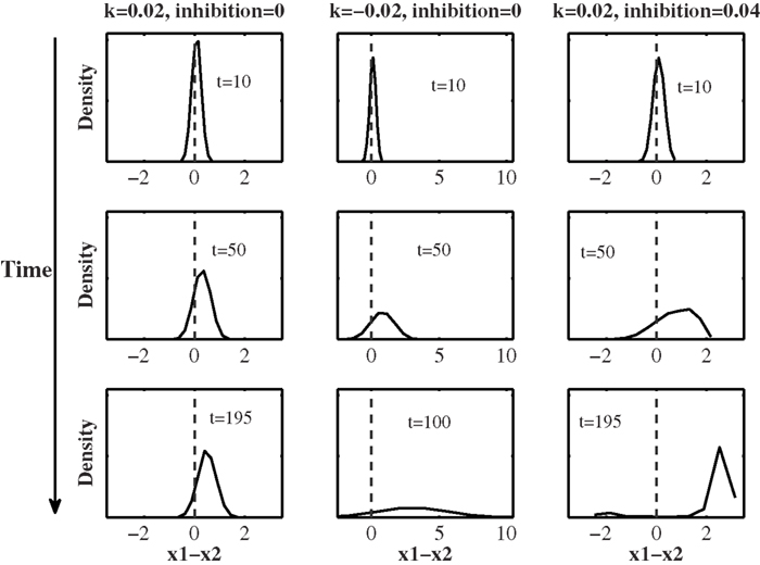
Figure 3. Time evolution of the decision variable x = x1 − x2 in three different leak-inhibition conditions. Adapted with permission from Usher and McClelland (2001).
On the other hand, when inhibition dominates leak in the full model, k < β, the quantity (k − β) inEq.3 becomes negative; taking this together with the minus sign in front of the (k − β)x term, we see that net effect of leak and inhibition becomes self excitation. In that case, any difference between the two decision variables will grow and explode with time. See Figure 3, middle column. Since early evidence has more time to grow than late information, early evidence overweighs late information in determining decisions, causing primacy. Although the mean and the standard deviation of the distribution in this condition both grow without bound as time increases, the resulting choice probability, determined by the ratio between the two, evolves and levels off with time in the same way in this condition as in the leak-dominant condition (see Usher and McClelland, 2001; Gao et al., 2011 for more details). Finally, when leak and inhibition are in perfect balance, k = β, neither leak nor self excitation occurs. The (k − β)x term disappears fromEq.3, and the model behaves as the drift-diffusion model (Bogacz et al., 2006; this case is not illustrated in the figure).
Non-linearity comes into play in the inhibition-dominant regime. According to the linear version of the LCA in Eq.3, the self excitation drives the evidence difference, x, to infinity with time. However, in the full LCA model, including the non-linearity at 0, once the losing unit’s activation reaches 0, it stops going further down and stops sending any inhibitory signal. The activity of the winning unit will be driven only by its leak and by its input (I1 or I2 depending on which unit is the winner). Therefore its activity, as well as the difference between its activity, levels off as further time passes. Figure 3, right column demonstrates the dynamics of the evidence difference variable x in this situation. Although the detailed dynamic of x in the non-linear model differs from that in the linear version, the choice probability distributions for the two models are very similar. This is because the non-linearity takes effect only after some time has passed. By this time, the amplification of early signals has already exerted its influence on the outcome (Usher and McClelland, 2001). Therefore, in the inhibition-dominant regime, both the full non-linear LCA and the linearized LCA produce a primacy pattern.
To illustrate the recency and primacy effects exhibited by the leak and inhibition-dominant LCA we performed the same reverse correlation analysis as in Figure 2, comparing leak-dominant and inhibition-dominant LCA with the BD model (Figure 4). Both alternatives (left/right) received noisy input for 200 simulation time-steps (Gaussian values with zero mean and SD of 0.1). BD was simulated with A = 0.8, inhibition-dominant LCA with k = 0.05, β = 0.095, I0 = 0.1 and leak-dominant LCA with k = 0.05, β = 0.025, I0 = 0.1. Larger differences between the left choice activity curve (blue) and the right choice activity curve (red) at the beginning of the trial indicates primacy, while larger differences at the end indicates recency. Figure 4 demonstrates that although the leak-dominant LCA (Figure 4C) results in recency, the inhibition-dominant LCA results in primacy (Figure 4B). The behavioral results reported in Kiani et al. (2008), although inconsistent with the leak-dominant LCA, are thus shown to be consistent with either the BD model or the inhibition-dominant LCA.
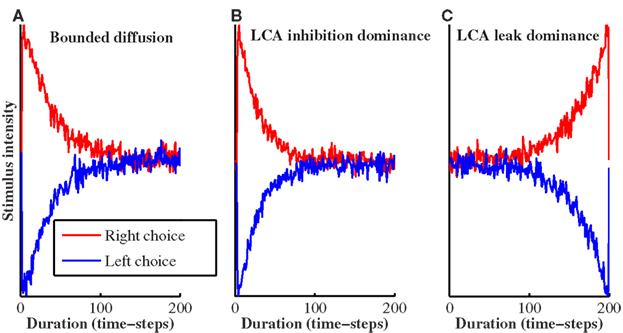
Figure 4. Reverse correlations for the bounded diffusion (A) and the leaky competing accumulators in inhibition-dominance (B), leak-dominance (C) models, showing the average input of the winning (red) and losing (blue) units, in zero-coherence simulated trials.
The rich dynamics of the LCA model also allows it, with certain settings of its parameters, to produce a transition between primacy and recency. In Figure 5A, we demonstrate such a case with the following values of the leak, inhibition and baseline parameters: k = 0.172, β = 0.748, I0 = 0.095, and σ = 0.1. We simulated a switch trial, where the motion coherence stays constant in magnitude throughout the trial but the direction switches in the middle. Inputs are I1 = 0.026, I2 = 0 for the first half of the trial and I1 = 0, I2 = 0.026 for the second half. We plot the probability of choices supported by the early half of the trial. A value above 0.5 implies early information determines the final decision more often than late information, i.e., primacy, and a value below 0.5 implies early information determines decisions less often than late information, i.e., recency. Each data point is based on simulations of 30,000 trials, and five durations were used consisting of 71, 157, 243, 329, and 414 time-steps. One can see a transition from primacy to recency as stimulus duration increases.
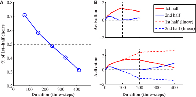
Figure 5. The transition from primacy-to-recency as stimulus duration increases. (A) Probability of choices toward the alternative supported in the first half of the trial in the switch condition. See text for parameter values. (B) Activity trajectories of the two accumulators when stimulus duration is short (top) and long (bottom). Red denotes the alternative supported in the first half of the trial, while blue denotes the alternative supported in the second half. In the bottom panel, we also plotted out the simulation results using the linear LCA (dashed lines).
In order to explain how the transition results from the LCA, we show activations of the two accumulators in a typical trial in Figure 5B. The red curve stands for the alternative supported in the first half of the trial, and the blue curve for the one supported in the second half. When stimulus duration is short (top panel), the accumulator associated with the red curve wins because the input during the first half of the trial leads it to suppress the other alternative, which does not have a chance to recover after the evidence reverses. At the time of the switch, the early-supported (red) accumulator is sending strong inhibition to the other accumulator (blue curve). Although the blue accumulator is supported by the stimulus input in the second half of the trial, its activation grows very slowly, rising only after the red accumulator’s activation has sufficiently decayed. This takes long enough so that the blue accumulator does not have a chance to win out. When stimulus duration is long (bottom panel, solid lines), the activity of the blue accumulator reaches zero well before the switch and stays pinned at this value. Following that, the activity of the red curve levels off; it no longer receives any inhibition from the other accumulator, but its activation levels off due to the effect of the leak. Therefore, although the first half of the trial in this case is much longer than that in the short duration scenario, the activity levels of the two accumulators are similar at the time of the switch. After the switch, the two curves evolve with time in the same manner as they do in the top panel. However, in this case, the activation of the red accumulator has more time to decay. The activation of the blue accumulator has more time to grow and its activation eventually comes to surpass the activation of the red alternative. Note that this transition from primacy to recency is caused by the interplay between the non-linearity at zero and the greater weight to early evidence caused by inhibition dominance. It does not occur in the linear case (dashed lines, lower panel of Figure 5B), nor does it occur with a high level of inhibition dominance.
In summary, primacy bias is consistent with both the BD and the inhibition-dominant LCA. However, LCA is also consistent with recency or balanced weighting of early vs. late evidence. A distinctive signature of the non-linear inhibition-dominant LCA is the transition from primacy at short durations to recency at long durations with some parameter settings. In the following section, we report the experimental findings of our studies, considering whether they exhibit features consistent with the greater flexibility of the LCA.
Experiment 1A
The experiment followed the procedures used in Kiani et al. (2008), as described in Section “Materials and Methods.” Observers were asked to determine the predominant direction of moving dots. While some dots were moving randomly, some were moving coherently either to the left or to the right. As in Kiani et al., we used four coherence levels and exponentially distributed stimulus durations in the range 150–1750 ms. Participants were trained to respond within a window of 300 ms following onset of the go cue in order to earn points. The critical manipulation of the evidence was applied in a subset of trials (80% of the trials with durations 300 ms or longer), in the form of a 200 ms “motion pulse” corresponding to a change in coherence of ±3.2%.
All of the observers learned to respond within the 300 ms response window and their accuracy increased with motion coherence according to a sigmoidal function (results from participant CS are shown in Figure 6A). As in Kiani et al. (2008), the pulse resulted in a shift of the psychometric curves. A logistic regression was performed to measure the size of the horizontal shift in units of coherence (see also Equation 4 in Kiani et al., 2008). Of special interest is that the effect size of the shift dropped as the pulse was applied later in the trial, indicating that early information has a larger effect on choices. To quantify this, we considered trials with durations of 700 ms or more, and divided the trials into three quantiles according to the time of the pulse (Figure 6C). Figure 6B shows that this primacy pattern was present in all participants, with some variability as the effect of the pulse weakens in later quantiles.
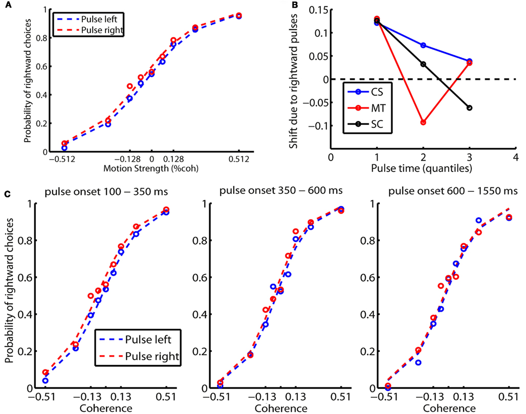
Figure 6. Results of experiment 1A with pulse perturbations. (A) The pulse results in a shift in the observer’s psychometric function. As an example, the result of CS is shown here. The percentage of rightward choices is plotted against rightward coherence levels. The red curve denotes rightward pulse and the blue curve denotes leftward pulse. (B,C) The effect size of the shift varies with the time of the pulse. (C) The psychometric function of participant CS as the pulse comes early, intermediate and late in the trial. (B) The effect size of the pulse in the unit of the equivalent motion coherence as a function of pulse time for all of the three observers.
Experiment 1B
Because the effect size in Experiment 1A is very small and therefore difficult to quantify, Experiment 1B was carried out in order to obtain a more robust measure of the temporal weighting profile. To do so, for each coherence and duration combination we created four conditions: (i) the constant condition, in which coherence stays fixed throughout the entire trial, (ii) the early condition, in which coherence is a fixed non-zero value during the first half of the trial and zero during the second half, (iii) the late condition, in which the coherence is zero in the first half of the trial and is a fixed non-zero value during the second half, and (iv) the switch condition, in which the coherence stays constant in magnitude but the direction of motion switches in the middle of the trial. The switch condition occurred only with the two low coherence levels to minimize the possibility of participants noticing the switch in motion direction. It is expected that the constant condition will result in higher choice accuracy, as it contains twice as much information as the early/late conditions. There are two critical tests. The first one is the accuracy level in the early condition relative to that in the late condition; and the second is the choice preference toward the alternative supported in the first half relative to that in the second half in the switch condition. A primacy pattern means higher accuracy in the early condition than in the late condition, and more choices toward the alternative supported in the first half of the trial. Recency means the opposite. The observations are shown in Figure 7.
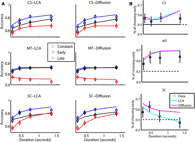
Figure 7. Results of experiment 1B. (A) Accuracy as a function of stimulus duration in the constant, early and late conditions. Left: Data (symbols) and the leaky competing accumulator fit (lines). Error bars correspond to 95% CI. Right: Data and bounded diffusion fit. (B) Predictions of the leaky competing accumulator (cyan) and bounded diffusion (magenta) in the switch condition. Parameters of the models are from the fitting in Panel A. Proportion of choices supported early in the trial was plotted against stimulus duration. Error bars correspond to 95% CI. Larger error bars are due to smaller sample size in the switch condition.
In Figure 7A, the accuracy averaged across coherence levels is displayed as a function of stimulus duration for the constant (blue), early (black), and late (red) conditions for the three observers. The results are also fitted by the LCA (left panel) and the BD (right panel) models. In all observers, accuracy increases with stimulus duration and the accuracy in the constant condition is higher than in the early and late conditions. More importantly, accuracy in the early condition is higher than in the late condition, implying a primacy effect. The size of the accuracy difference in the two conditions, however, varies among the three observers. It is very large in one of them (MT), who completely neglected late evidence except in the shortest lag condition, but is smaller in the other two. In SC, this difference also declines as stimulus duration lengthens. The interaction between the recency-primacy pattern and stimulus duration was consistent with the non-linear LCA model, but it provides a challenge to the BD model as shown below.
Quantitative measures of goodness of fit are shown for the LCA and BD models in Table 1. We used BIC, which takes the number of degrees of freedom into account, to measure the goodness of fit. BD and LCA fit the data of CS and MT equally well, while LCA provides a better fit to the data from SC – the participant who showed an interaction between the primacy effect and stimulus duration.
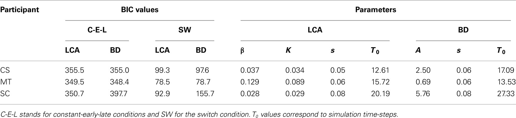
Table 1. Bayesian information criterion values and model parameters for the LCA and BD models for the three subjects in experiment 1B.
In Figure 7B, we plotted choice probabilities toward the alternative supported in the first half of the trial. A value above 0.5 means primacy, while a value below 0.5 means recency. Consistent with the results in the early/late conditions, the switch condition also reveals a clear primacy in CS and MT, and this effect is particularly strong in MT. For SC, we see a primacy pattern when stimulus duration is short, and it disappears and even reverses to a recency pattern as the stimulus duration lengthens. Due to its smaller data size, we did not use the switch condition in model fitting. Rather, we adopted the parameters from the fitting of the constant/early/late condition and plotted the model predictions in the switch condition (solid lines in Figure 7B). Again, both models fit the first two participants about equally well, but BD does not fit the data of SC as well as LCA does.
Experiments 2A and 2B
Both versions of Experiment 1 replicate the primacy bias reported by Kiani et al. (2008). Since the results of Experiment 1B and the data fitting we conducted showed that it was not possible in two of the three participants to discriminate the two models using fits of the data, we chose in our second set of experiments to focus on the detection of the qualitative pattern of data that can discriminate the models (Figure 5). While this pattern only arises at a particular set of LCA parameters, it is special because it goes against what a BD model can predict. In particular, we wished to examine whether any of the observers show a transition from primacy-to-recency, which is a signature prediction of the non-linear LCA model and is a challenge to the BD model.
A further goal of our second experiment is to examine if the primacy bias observed in Experiment 1 can be reversed or attenuated. Although the primacy bias seems to be a robust observation (Kiani et al., 2008), it is possible that it may be task-dependent. The time pressure in Experiment 1, is very high, to an extent that is similar to, and perhaps even more extreme than that in Kiani et al. (see text footnote 5). Under such circumstances, decision makers presumably need to be ready to make a prompt response when the go cue comes; this could promote either a lower decision bound for the BD model or stronger lateral inhibition in the LCA.
In order to investigate this question, we relaxed the time pressure in our remaining experiments. First, we relaxed the response window after the go cue from 300 ms to 1 s. This allowed observers enough time to prepare their response after the go cue. Second, we used uniformly distributed stimulus durations instead of exponentially distributed durations. This way, long stimulus durations are equally likely as short stimulus durations (see Discussion for further consideration of this issue).
As in Experiment 1, each participant was tested for several sessions to provide statistical power (see Materials and Methods). In total seven observers were tested with this procedure. The first four participants were tested in Experiment 2A with stimulus durations of 150–1750 ms. After noticing that their accuracy levels differed dramatically, we adapted the difficulty level individually and employed a wider range of stimulus durations (150–2350 ms) for another three participants.
The results are summarized in Figure 8A. The average primacy score, defined as the average accuracy level in the early condition minus that in the late condition, drops dramatically from Experiment 1B to Experiment 2A and 2B. Since there is no significant difference in procedure or results between the participants in 2A and 2B, we collapse these two groups into one, and refer to this as Experiment 2. The primacy score was significantly larger in Experiment 1B than in Experiment 2 [11 vs. 2%; t(8) = 2.98; p < 0.02]. While all the observers in the Experiment 1B showed the primacy effect, there was considerable variation among observers in the second group. We therefore conducted a subject-by-subject ANOVA on the main effect of early vs. late and on the interaction between the size of this effect and the stimulus duration. To carry out this analysis, we divided the data of each observer into mini-sessions or quasi-subjects that corresponded to all of the session-by-coherence combinations. Each such quasi-subject contributed an equal number of trials to the relevant dependent variables of duration and condition (early vs. late), factoring out the common variability related to fatigue, practice, or performance levels. We thus subjected the mini-session data to a repeated-measure (4 × 2) ANOVA, with 4 levels of trial duration and 2 levels of timing within trial (early vs. late). The ANOVA results are summarized in Table 2.
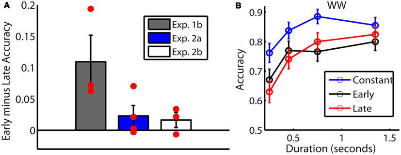
Figure 8. Results of experiment 2. (A) Primacy scores of all the participants in experiments 2A and 2B in comparison to those in Experiment 1B. The primacy score is calculated as the accuracy in the early minus that in the late condition, averaged across all coherences and all stimulus durations. Red circles correspond to individual data. Error bars correspond to 1 SE. (B) Accuracy as a function of stimulus duration for participant WW in Experiment 2A. Constant, early, and late conditions are shown in blue, black, and red respectively. Error bars correspond to 95% CI.
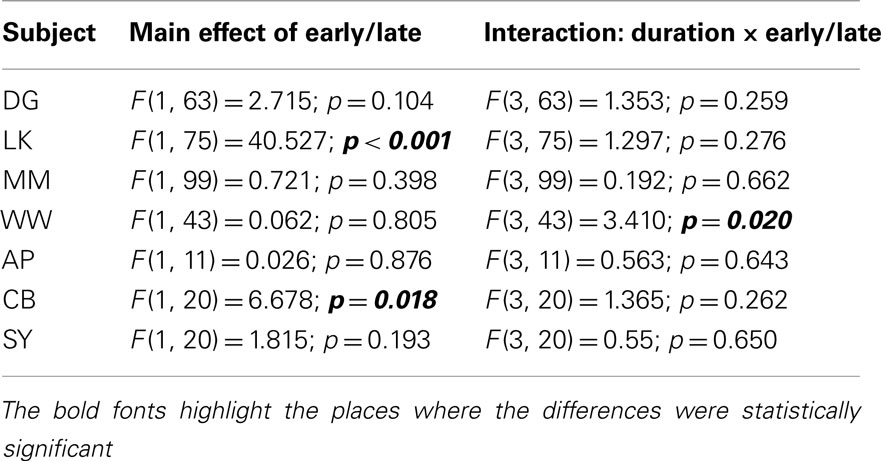
Table 2. Results of ANOVA examining the effect of timing within trial (early vs. late) and its interaction with trial duration for all participants in experiments 2A and 2B.
Table 2 revealed that only two of the seven observers (LK and CB) showed a significant main effect of primacy. More interestingly, participant WW showed a significant interaction between temporal weighting and duration (Figure 8B). WW’s decisions were mainly driven by early information when stimulus duration was short, while they were driven by late information when stimulus duration was long. This transition from primacy-to-recency is a signature of the non-linear LCA model and it is not consistent with the BD model. Please refer to the Appendix for detailed individual data for all seven participants (Figure A3).
Discussion
Stimulated by the recent study of Kiani et al. (2008), we have examined the temporal weighting of evidence in decision making using a time-controlled protocol. In both of the tested monkeys, Kiani et al. found a primacy bias – early information was more important in decision making – and they proposed the BD model as the mechanistic basis for this observation. According to this model, observers make a decision when a decision bound is reached and ignore any information afterward. In Experiment 1 we examined two types of evidence manipulations: brief motion pulses (or perturbations; see also Huk and Shadlen, 2005) and larger within trial evidence changes at the middle of the stimulus duration. The two methods gave similar results, indicating primacy, though the effect of the latter manipulation was more robust. In our first pair of experiments (1A and 1B), we used a procedure with high time pressure, similar to Kiani et al. In the second pair of experiments (2A and 2B), we relaxed the time pressure by allowing slower responses after the go cue and by using relatively more long trials. Experiments 1A and 1B replicated the primacy bias reported by Kiani et al. while in Experiments 2A and 2B the primacy bias significantly diminished. With some participants, we also found that primacy bias drops, or even transitions to recency (with a stronger weight to late evidence relative to early evidence) as stimulus duration lengthens. We showed that the LCA model can account for the primacy bias as well as the BD model, and that it can also capture the transition from primacy to recency, a pattern that poses a challenge to the BD model.
The LCA model does not assume the presence of a decision bound in the time-controlled paradigm. In this model, accuracy levels off due to the imbalance between the leak and the inhibition, and the time scale of this process is determined by the absolute value of the difference between the strength of the leak and the strength of the inhibition. The sign of this difference, although it does not affect the overall time-accuracy profile, has a profound effect on the relative weight of early vs. late evidence (Usher and McClelland, 2001; Gao et al., 2011). Unlike in the leak-dominant LCA, which gives a higher weight to late evidence, the inhibition-dominant LCA gives a higher weight to early evidence. Thus, this framework, as well as the attractor model (Wang, 2002)4, provides an alternative to the BD model’s account of the primacy pattern. The LCA and related models are also consistent with aspects of the results of an earlier perturbation study by Huk and Shadlen (2005). In this study, the effect of a transient change in evidence on activity in putative evidence accumulation neurons in area LIP is higher when applied early during the observation interval, and becomes very weak near the end (Huk and Shadlen, 2005; Figure 10B). The authors attempted to fit these results using the BD model and noted that it did not explain the very weak impact of later pulses on the neuron’s responses (p. 3027). These authors suggested the attractor model of Wang (2002) as one mechanism that could account for the residual effect. In Figure 9, we present an informal simulation showing that the inhibition-dominant LCA can also capture the pattern Huk and Shadlen (2005) found in their data. Like neurons in LIP, the accumulators in the LCA are highly sensitive to motion pulses occurring early in a stimulus presentation period, and this effect becomes progressively weaker as integration time continues.
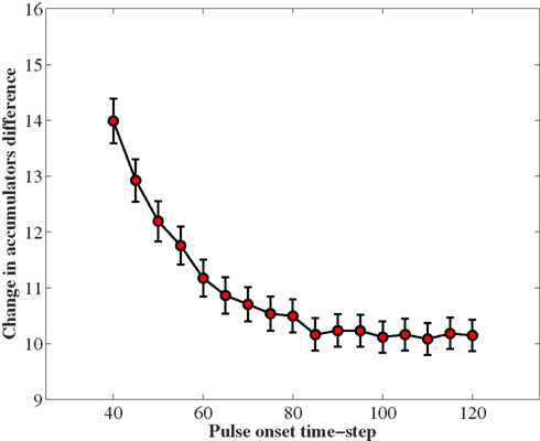
Figure 9. The effect of a short pulse on the activation states of two leaky competing accumulators, at different times in the trial. Each trial lasted for 200 time-steps. The two accumulators received Gaussian inputs with mean and standard deviation both equal to 1. The pulse was inserted for 40 time-steps and increased the mean input to the target accumulator by 1 unit. In the y-axis we plot the change that the pulse conferred to the difference between the target and the non-target accumulator. The change is calculated by subtracting the difference between the accumulators’ activity 40 time-steps after the offset of the pulse minus the activity difference at the onset of the pulse. The effect diminishes as the time of the pulse onset increases. The leaky competing accumulator model was simulated with inhibition three times larger than the leakage (β = 0.15, k = 0.05). Error bars correspond to 95% CI.
The main result of Experiment 2 was a reduction in the primacy bias, compared to Experiment 1. This difference in the temporal weighting of evidence can be understood in relation to two procedural differences between the two experiments. The first change is that the response window was relaxed from 300 to 1000 ms. With a 300 ms response window, participants must be prepared to respond very quickly once the go cue comes. Under the BD model, this time pressure could lead them to adopt a lower decision bound, so that they will be ready to respond when the go cue occurs. Similarly, under the LCA, this time pressure could encourage adjusting the strength of lateral inhibition, since stronger inhibition helps to encourage a difference in the activation of the two accumulators, which may facilitate faster responding (Gao et al., 2011; Gao and McClelland, in preparation). In any case, time pressure may be one factor contributing to the strong primacy pattern observed in our Experiment 1 and in Kiani et al. (2008) 5.
The second experimental change is that we used uniformly distributed stimulus durations rather than exponentially distributed durations. The reason Kiani et al. (2008) used exponentially distributed stimulus durations was to ensure that observers have no information about the time when the go cue would appear. This choice, however, results in much more frequent short trials than long trials. This factor could encourage participants to ensure they are ready to respond early in the trial, a factor that could further encourage a primacy bias. The empirical findings of our study suggest two potential reasons why Kiani et al. found only primacy while the study of Usher and McClelland (2001) found all three patterns of primacy, recency, and balanced integration. Like in Experiment 2, participants in the Usher and McClelland study were not presented with predominantly short stimuli, or a short deadline. Our findings also suggest that time pressure, exerted by a narrow response window and/or by more short trials, is one of the factors determining the relative importance of information at different time points.
The results of these experiments also show important individual differences (see also Usher and McClelland, 2001). We were particularly interested in examining whether observers show a transition from primacy, when stimulus duration is short, to recency, when stimulus duration is long. This signature prediction of the inhibition-dominant LCA is challenging for the BD model. Such a transition was found in the performance of subject WW in Experiment 2A, and a similar pattern was found in observer SC in Experiment 1B. Despite detecting the predicted signature of the non-linear LCA, we believe that any conclusions at this stage should be tentative, since they are only supported by the data from 2 of 10 participants.
Further experimentation with additional observers and experimental protocols will be needed to more thoroughly examine the relative merits of the BD and LCA models and to delineate in more detail the conditions under which recency as well as primacy patterns might be obtained. This is important because a number of other experimental paradigms have shown recency patterns (Pietsch and Vickers, 1997; Usher and McClelland, 2001; Newell et al., 2009). Note also that here we only examined temporal weighting of perceptual evidence in a time-controlled paradigm. Although more challenging (since one cannot plan a mid-point evidence change when RT is under subject control), the examination of temporal evidence is also possible in the free-response paradigm. Recently, Zhou et al. (2009) have developed a sophisticated perturbation protocol that can distinguish between a number of competing choice-RT-models in conditions of high signal-to-nose (low error-rate). Future work with such perturbation protocols as well as with balanced or non-balanced evidence switches (e.g., 40% left vs. 60% right) are vital to fully understand the details of the mechanisms of decision making, as are investigations that collect enough data per participant to reliably explore individual differences.
One additional factor that may explain the difference in temporal profile obtained in this study and that in Kiani et al. (2008), compared to studies that showed recency effects is the degree of practice. Practice is quite extensive in our studies as well as in the Kiani study. One possibility, suggested by Brown and Heathcote (2005), is that practice increases the efficiency of evidence accumulation by reducing the effective leak. This factor could play a role in the comparison between our Experiment 1 and 2 as well, since participants in Experiment 1 had more practice, on average, than those in Experiment 2.
Kiani et al. (2008) proposed that bounded integration is a universal decision principle that applies not only to self-paced decisions but also to tasks in which the duration of evidence accumulation is controlled by the experimenter. The results we report here, taken together with other studies showing recency effects, suggest that this conclusion should be reconsidered. Interestingly, one of the motivations suggested by Kiani and colleagues against leaky integration was the idea that leaky integration might be maladaptive in that it discards some of the evidence. While this may be true in some conditions, it is also true that placing a bound on information integration also disregards important decision-relevant information6. It might be supposed that unbounded integration (achieved in the drift-diffusion model without a bound or by a linear version of the LCA with a perfect balance between leak and inhibition) would always be the best policy, but this may ignore important contingencies that could make a recency vs. a primacy strategy more adaptive. These contingencies include the need to be ready to respond quickly and the need to be sensitive to a change in evidence as well as other factors.
We propose that the mechanism in play in the non-linear inhibition-dominant LCA has the advantage of prioritizing early information in a flexible and reversible manner. Interestingly, while the non-linearity reduces the optimality of the model in choices between two alternatives, it has the advantage of making the mechanism more optimal and robust when there is a larger number of alternatives (Bogacz et al., 2007). In other work in our labs, this mechanism is supported by data showing that responses triggered by a go cue are faster for correct than incorrect choices (Gao and McClelland, in preparation) and also by decision biases in favor of alternatives whose evidence is temporally anti-correlated with evidence for other alternatives (Tsetsos et al., 2011). Yet other work indicates that some participants exhibit the bimodal decision states like these exhibited by the inhibition-dominant LCA (as illustrated in Figure 3, right column; Lachter et al., 2011).
In closing, we suggest that the principles that are at play in the LCA – leaky integration and lateral inhibition – may generalize beyond the domain of evidence based decisions that we have focused on here. These principles, inspired by known properties of neural systems (Usher and McClelland, 2001), are also found in the attractor model of Wang (2002), and in models based on Decision Field Theory, an approach that has been successfully applied to various aspects of preference based decisions, such as risky choice (Busemeyer and Townsend, 1993; Johnson and Busemeyer, 2005), and to several distinctive characteristics of performance in multi-attribute, multi-alternative decisions (Roe et al., 2001; Usher and McClelland, 2004; Tsetsos et al., 2010).
Author Contributions
Juan Gao and James L. McClelland designed and performed the experiments. Marius Usher, Konstantinos Tsetsos, Juan Gao, and James L. McClelland developed theoretical ideas. Konstantinos Tsetsos, Marius Usher, and Juan Gao analyzed the data and conducted model simulations. Marius Usher, Konstantinos Tsetsos, Juan Gao, and James L. McClelland wrote the paper.
Conflict of Interest Statement
The authors declare that the research was conducted in the absence of any commercial or financial relationships that could be construed as a potential conflict of interest.
Acknowledgments
This research was supported by Air Force Research Laboratory Grant FA9550-07-1-0537. We thank the reviewers for helpful comments and we thank Jenica Law for proofreading the manuscript.
Footnotes
- ^The data set is available at: http://www.stanford.edu/group/pdplab/projects/Frontiers2012/.
- ^Due to a programming error, the direction of motion in the first half of each switch trial was treated as correct in the first session for participants MT and CS.
- ^These equations correspond to discrete versions of the differential Equations ; with the following correspondences with the parameters in the finite difference equations: In the simulations, dt = 0.0035 s (3.5 ms) and the reported parameter values are those in the finite difference equations.
- ^The attractor model was not directly simulated in relation to the temporal weighting of evidence, but we expect it to have similar predictions as the inhibition-dominant LCA, as both have unstable Ornstein–Uhlenbeck dynamics.
- ^We note that in Kiani et al. (2008), a delay period was included in half of the trials after the stimulus offset. However, trials with and without delays were mixed randomly within blocks, making it necessary for the animal to be ready to respond promptly at the termination of the stimulus, which was very brief on many trials. The response window was 500 ms in Kiani et al. as compared with only 300 ms in our Experiment 1. We conducted a small experiment with a 500 ms response window and found that the primacy bias was not distinguishable in the 500 ms and the 300 ms conditions.
- ^We do not argue against the idea that decision boundaries are sometimes used even when the stimulus duration is experimentally controlled (Ratcliff, 2006). However, we suspect that such boundaries should be under subject control, and reflect a variety of experimental demands (such as speed-accuracy trade-offs) and contingencies (such as information about expected stimulus durations). Additionally, the bound should be soft rather than rigid.
References
Bogacz, R., Brown, E., Moehlis, J., Holmes, P., and Cohen, J. D. (2006). The physics of optimal decision making: a formal analysis of models of performance in two-alternative forced-choice tasks. Psychol. Rev. 113, 700–765.
Bogacz, R., and Cohen, J. D. (2004). Parameterization of connectionist models. Behav. Res. Methods 36, 732–741.
Bogacz, R., Usher, M., Zhang, J. X., and McClelland, J. L. (2007). Extending a biologically inspired model of choice: multi-alternatives, nonlinearity and value-based multidimensional choice. Philos. Trans. R. Soc. Lond. B Biol. Sci. 362, 1655–1670.
Brown, S. D., and Heathcote, A. (2005). Practice increases the efficiency of evidence accumulation in perceptual choice. J. Exp. Psychol. Hum. Percept. Perform. 31, 289–298.
Burr, D. C., and Santoro, L. (2001). Temporal integration of optic flow, measured by contrast and coherence thresholds. Vision Res. 41, 1891–1899.
Busemeyer, J. R., and Townsend, J. T. (1993). Decision field theory: a dynamic cognition approach to decision making. Psychol. Rev. 100, 432–459.
Ditterich, J. (2010). A comparison between mechanisms of multi-alternative perceptual decision making: ability to explain human behavior, predictions for neurophysiology, and relationship with decision theory. Front. Neurosci. 4:184. doi:10.3389/fnins.2010.00184
Gao, J., Tortell, R., and McClelland, J. L. (2011). Dynamic integration of reward and stimulus information in perceptual decision-making. PLoS ONE 6, e16749. doi:10.1371/journal.pone.0016749
Gold, J. I., and Shadlen, M. N. (2000). Representation of a perceptual decision in developing oculomotor commands. Nature 404, 390–394.
Gold, J. I., and Shadlen, M. N. (2001). Neural computations that underlie decisions about sensory stimuli. Trends Cogn. Sci. (Regul. Ed.) 5, 10–16.
Gold, J. I., and Shadlen, M. N. (2002). Banburismus and the brain: decoding the relationship between sensory stimuli, decisions, and reward. Neuron 36, 299–308.
Gold, J. I., and Shadlen, M. N. (2007). The neural basis of decision making. Annu. Rev. Neurosci. 30, 535–574.
Hanes, D. P., and Schall, J. D. (1996). Neural control of voluntary movement initiation. Science 274, 427–430.
Horwitz, G. D., and Newsome, W. T. (2001). Target selection for saccadic eye movements: prelude activity in the superior colliculus during a direction-discrimination task. J. Neurophysiol. 86, 2543–2558.
Huk, A. C., and Shadlen, M. N. (2005). Neural activity in macaque parietal cortex reflects temporal integration of visual motion signals during perceptual decision making. J. Neurosci. 25, 10420–10436.
Johnson, J. G., and Busemeyer, J. R. (2005). A dynamic, computational model of preference reversal phenomena. Psychol. Rev. 112, 841–861.
Kiani, R., Hanks, T. D., and Shadlen, M. N. (2008). Bounded integration in parietal cortex underlies decisions even when viewing duration is dictated by the environment. J. Neurosci. 28, 3017–3029.
Lachter, J., Corrado, G. S., Johnston, J. C., and McClelland, L. L. (2011). “Distribution of confidence ratings for a simple perceptual task,” in the 52nd Annual Meeting of the Psychonomic Society, Seattle.
Mazurek, M. E., Roitman, J. D., Ditterich, J., and Shadlen, M. N. (2003). A role for neural integrators in perceptual decision making. Cereb. Cortex 13, 1257–1269.
Newell, B. R., Wong, K. Y., Cheung, J. C. H., and Rakow, T. (2009). Think, blink or sleep on it? The impact of modes of thought on complex decision making. Q. J. Exp. Psychol. 62, 707–732.
Pietsch, A. J., and Vickers, D. (1997). Memory capacity and intelligence: novel techniques for evaluating rival models of a fundamental information-processing mechanism. J. Gen. Psychol. 199, 229–339.
Ratcliff, R., Hasegawa, Y. T., Hasegawa, R. P., Smith, P. L., and Segraves, M. A. (2007). Dual diffusion model for single-cell recording data from the superior colliculus in a brightness-discrimination task. J. Neurophysiol. 97, 1756–1774.
Ratcliff, R., and McKoon, G. (2008). The diffusion decision model: theory and data for two-choice decision tasks. Neural Comput. 20, 873–922.
Ratcliff, R., and Rouder, J. N. (1998). Modeling response times for two-choice decisions. Psychol. Sci. 9, 347–356.
Ratcliff, R., and Smith, P. L. (2004). A comparison of sequential sampling models for two-choice reaction time. Psychol. Rev. 111, 333–367.
Roe, R. M., Busemeyer, J. R., and Townsend, J. T. (2001). Multialternative decision field theory: a dynamic connectionist model of decision making. Psychol. Rev. 108, 370.
Roitman, J. D., and Shadlen, M. N. (2002). Response of neurons in the lateral intraparietal area during a combined visual discrimination reaction time task. J. Neurosci. 22, 9475–9489.
Rorie, A. E., Gao, J., McClelland, J. L., and Newsome, W. T. (2010). Integration of sensory and reward information during perceptual decision-making in lateral intraparietal cortex (LIP) of the macaque monkey. PLoS ONE 5, e9308. doi:10.1371/journal.pone.0009308
Shadlen, M. N., and Newsome, W. T. (2001). Neural basis of a perceptual decision in the parietal cortex (area LIP) of the rhesus monkey. J. Neurophysiol. 86, 1916–1936.
Tsetsos, K., Usher, M., and Chater, N. (2010). Preference reversal in multiattribute choice. Psychol. Rev. 117, 1275–1291.
Tsetsos, K., Usher, M., and McClelland, J. L. (2011). Testing multi-alternative decision models with non-stationary evidence. Front. Neurosci. 5:63. doi:10.3389/fnins.2011.00063
Usher, M., and McClelland, J. L. (2001). The time course of perceptual choice: The leaky, competing accumulator model. Psychol. Rev. 108, 550–592.
Usher, M., and McClelland, J. L. (2004). Loss aversion and inhibition in dynamical models of multialternative choice. Psychol. Rev. 111, 757–769.
van Ravenzwaaij, D., van der Maas, H. L. J., and Wagenmakers, E.-J. (2012). Optimal decision making in neural inhibition models. Psychol. Rev. 119, 201–215.
Wald, A. (1946). Differentiation under the expectation sign in the fundamental identity of sequential analysis. Ann. Math. Stat. 17, 493–497.
Wang, X. J. (2002). Probabilistic decision making by slow reverberation in cortical circuits. Neuron 36, 955–968.
Wickelgren, W. A. (1977). Speed-accuracy tradeoff and information processing dynamics. Acta Psychol. (Amst.) 41, 67–85.
Wong, K. F., Huk, A. C., Shadlen, M. N., and Wang, X. J. (2007). Neural circuit dynamics underlying accumulation of time-varying evidence during perceptual decision making. Front. Comput. Neurosci. 1:6. doi:10.3389/neuro.10.006.2007
Wong, K. F., and Wang, X. J. (2006). A recurrent network mechanism of time integration in perceptual decisions. J. Neurosci. 26, 1314.
Zhou, X., Wong-Lin, K.-F., and Holmes, P. (2009). Time-varying perturbations can distinguish among integrate-to-threshold models for perceptual decision-making in reaction time tasks. Neural Comput. 21, 2336–2362.
Appendix
Perturbation Protocol in Experiment 1A
In experiment 1A, a momentary change (or pulse) in the motion coherence was introduced in 80% of the trials with duration longer than 300 ms. The motion pulse could be inserted between 100 ms after the beginning of the stimulus and 200 ms before it ended. Figure A1 illustrates the perturbation protocol: T ms after the stimulus onset (100 ms < T < Toverall − 200 ms) the motion coherence which previously equaled to a, increased by p (i.e., coherence level during the pulse was a + p, with p = ±3.2%). The duration of the pulse was ΔT = 200 ms.
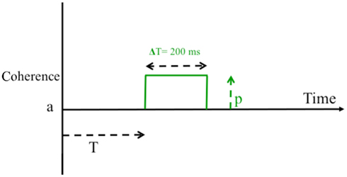
Figure A1. Illustration of perturbation protocol in Experiment 1B. After T ms the motion coherence level changes from a to a + p for a duration of 200 ms.
Excluded Sessions in Experiment 1B
For participants CS and MT the first session was discarded due to a programming mistake (see text footnote 2). Participants CS and SC had high and stable mean accuracy for all sessions (SD of accuracy was 2.2 and 3% respectively) and therefore we used 13 (after excluding the first session) and 12 sessions correspondingly. For participant MT the performance was unstable during the first 10 sessions (see Figure A2). These sessions were not included in the analysis, resulting in 9 analyzed sessions (the SD of accuracy for the first 10 sessions was 5%; after excluding these sessions SD was 1.7% for the remaining 9 sessions).
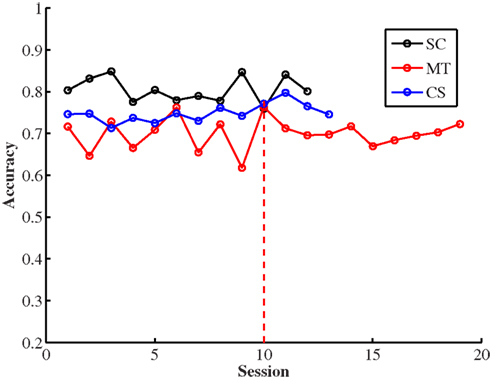
Figure A2. Mean accuracy as a function of session for the three subjects in Experiment 1B. For SC and CS, whose performance was relatively high and stable, all sessions were maintained for the analysis. For subject MT the sessions 1–10 (up to the red vertical line) were eliminated because the participant’s accuracy was unstable.
Individual Results from Experiment 2A and 2B
In Figure A3 the results of all participants (4 for Experiment 2A and 3 for Experiment 2B) are presented. Table 2 in the main text shows the statistical analysis performed on each subject regarding the direction of the timing effect (primacy/recency) and its interaction with the trial duration. Participants LK and CB showed a significant primacy while participant WW showed a significant interaction between primacy/recency and trial duration. This interaction is uniquely predicted by the LCA model (see Experiment 1A). The patterns exhibited by the other participants do not discriminate between the models.
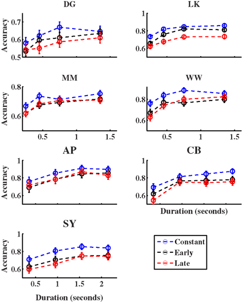
Figure A3. Accuracy as a function of stimulus duration and condition in Experiment 2A (participants DG, LK, MM, and WW) and Experiment 2B (adaptive condition; participants AP, CB, and SY). Error bars correspond to 95% CI.
Keywords: bounded diffusion, LCA, perceptual choice, non-stationary evidence, order effects
Citation: Tsetsos K, Gao J, McClelland JL and Usher M (2012) Using time-varying evidence to test models of decision dynamics: bounded diffusion vs. the leaky competing accumulator model. Front. Neurosci. 6:79. doi: 10.3389/fnins.2012.00079
Received: 09 December 2011; Accepted: 11 May 2012;
Published online: 12 June 2012.
Edited by:
David Albert Lagnado, University College London, UKReviewed by:
Alexander C. Huk, The University of Texas at Austin, USAEric-Jan Wagenmakers, University of Amsterdam, Netherlands
Joseph G. Johnson, Miami University, USA
Copyright: © 2012 Tsetsos, Gao, McClelland and Usher. This is an open-access article distributed under the terms of the Creative Commons Attribution Non Commercial License, which permits non-commercial use, distribution, and reproduction in other forums, provided the original authors and source are credited
*Correspondence: Konstantinos Tsetsos, Department of Experimental Psychology, University of Oxford, South Parks Road, Oxford, OX1 3UD, UK. e-mail:a29uc3RhbnRpbm9zLnRzZXRzb3NAcHN5Lm94LmFjLnVr; Marius Usher, Department of Social Sciences, School of Psychology and Sagol School of Neuroscience, Tel-Aviv University, Tel-Aviv 69978, Israel. e-mail:bWFyaXVzQHBvc3QudGF1LmFjLmls
†Konstantinos Tsetsos and Juan Gao have contributed equally to this work.