 Da Ma1,2,3*†
 Holly E. Holmes2†
 Manuel J. Cardoso1,4
 Marc Modat1,4
 Ian F. Harrison2
 Nick M. Powell1,2James M. O’Callaghan2
 Ozama Ismail2Ross A. Johnson5
 Michael J. O’Neill6Emily C. Collins5
 Mirza F. Beg5
 Karteek Popuri5
 Mark F. Lythgoe2‡
 Sebastien Ourselin1,4‡
- 1Translational Imaging Group, Centre for Medical Image Computing, University College London, London, United Kingdom
- 2Centre for Advanced Biomedical Imaging, University College London, London, United Kingdom
- 3School of Engineering Science, Simon Fraser University, Burnaby, BC, Canada
- 4School of Biomedical Engineering and Imaging Sciences, King’s College London, London, United Kingdom
- 5Tailored Therapeutics, Eli Lilly and Company, Lilly Corporate Center, Indianapolis, IN, United States
- 6Eli Lilly & Co. Ltd., Erl Wood Manor, Windlesham, United Kingdom
Brain volume measurements extracted from structural MRI data sets are a widely accepted neuroimaging biomarker to study mouse models of neurodegeneration. Whether to acquire and analyze data in vivo or ex vivo is a crucial decision during the phase of experimental designs, as well as data analysis. In this work, we extracted the brain structures for both longitudinal in vivo and single-time-point ex vivo MRI acquired from the same animals using accurate automatic multi-atlas structural parcellation, and compared the corresponding statistical and classification analysis. We found that most gray matter structures volumes decrease from in vivo to ex vivo, while most white matter structures volume increase. The level of structural volume change also varies between different genetic strains and treatment. In addition, we showed superior statistical and classification power of ex vivo data compared to the in vivo data, even after resampled to the same level of resolution. We further demonstrated that the classification power of the in vivo data can be improved by incorporating longitudinal information, which is not possible for ex vivo data. In conclusion, this paper demonstrates the tissue-specific changes, as well as the difference in statistical and classification power, between the volumetric analysis based on the in vivo and ex vivo structural MRI data. Our results emphasize the importance of longitudinal analysis for in vivo data analysis.
Introduction
In neuroimaging studies, quantitative analysis of neuroanatomy, such as volumetric analysis of brain structures extracted from magnetic resonance imaging (MRI) data sets, plays a crucial role in the diagnosis of diseases at the early stages of pathology before the onset of clinical symptoms (McEvoy and Brewer, 2010). This has been facilitated by automated analysis techniques such as atlas-based parcellation, which enable large data sets to be analyzed in a time efficient and unbiased manner. The application of MRI to study mouse models is increasingly being utilized to understand disease mechanisms as well as potential treatment effects, and a number of mouse brain MRI atlases are currently in existence to facilitate structural analysis of these models (Ma et al., 2005, 2008, 2014; Bai et al., 2012). However, whether to acquire data in vivo or ex vivo is always a debatable question during experimental design. For brains scanned ex vivo, there are no motion artifacts, and the prolonged scanning time enables (1) increased image resolution (leading to less partial volume effects), (2) improved signal to noise ratio, and (3) enhanced tissue contrast (Montie et al., 2010; Lerch et al., 2012; Holmes et al., 2017). The quality of images acquired ex vivo can be further enhanced using high concentrations of contrast-enhancement agents such as Gadolinium (Cleary et al., 2011). The enhancement of image quality in the ex vivo data can increase the statistical power to detect subtle volume changes when performing cross-sectional comparison between normal and disease groups (Lerch et al., 2012). However, samples prepared for ex vivo imaging suffer from morphological disruption to the tissues during processes such as fixation and perfusion (Lavenex et al., 2009). On the other hand, most of the intrinsic physiological and pathological characteristics of the animal’s tissues can be preserved if they are imaged in vivo (Schulz et al., 2011). Furthermore, with in vivo imaging, it is possible to trace the morphological changes of each individual animal longitudinally. This is especially important for monitoring disease progression (Zhang et al., 2010), as well as potential treatment effects over time using transgenic mouse models (Santacruz et al., 2005; Holmes et al., 2016). The trade-offs between longitudinal in vivo and cross-sectional ex vivo imaging data are an important factor to be consider during experimental design.
Our current understanding of volume changes from in vivo to ex vivo is inconclusive. Studies show inconsistent results on both clinical (Schulz et al., 2011; Kotrotsou et al., 2014) and preclinical imaging data (Ma et al., 2005, 2008; Zhang et al., 2010; Oguz et al., 2013). Lerch et al. (2012) measured the theoretical statistical power to compare in vivo and ex vivo imaging. Meanwhile, Holmes et al. (2017) investigated the effect size and sample size required for data analysis using tensor-based morphometry (TBM). In this study, we aim to further study and compare the volumetric analysis of individual structures using either longitudinal in vivo data or single-time-point ex vivo data acquired on the same animals.
Accurate structural parcellation is crucial for volumetric analysis. Conventional methods used to obtain volumetric information for regions-of-interest (ROIs) routinely implement manual delineation methods, which are both time-consuming and prone to human error (Ma et al., 2005; Richards et al., 2011). Comparatively, automatic structural parcellation has been continually improved and increasingly adopted to overcome the disadvantages of manual methods (Calmon and Roberts, 2000; Sharief et al., 2008; Almhdie-Imjabber et al., 2010). Recently, multi-atlas based techniques have been shown to provide highly accurate structural volumes in both clinical and preclinical studies (Rohlfing et al., 2004; Warfield et al., 2004; Aljabar et al., 2007; Cardoso et al., 2013; Ma et al., 2018).
In this study, we compared structural volumetric information extracted from both in vivo and ex vivo mouse brain data sets using a fully automated multi-atlas structural parcellation framework (Ma et al., 2014). We sought to explore how changes in volumes between in vivo and ex vivo in the mouse brain are distributed across different brain tissues and structures; whether the difference varies across different strains and treatment; and whether those variations within structures affect the statistical and classification power when comparing volumetric differences with expected pathology changes of brain atrophy with and without drug treatment. We also investigated whether including longitudinal information can improve the analysis of group differences.
Materials and Methods
Experimental Data
We used the rTg4510 transgenic mouse strain, which faithfully recapitulates several key features of clinical Alzheimer’s disease (AD) and frontal temporal dementia (FTD) including progressive atrophy of the forebrain regions and the accumulation of neurofibrillary tangles of tau (NFTs) (Santacruz et al., 2005). The NFT overexpression level and accompanying volumetric brain changes in the rTg4510 mouse can be attenuated using doxycycline, (Holmes et al., 2016); thus, this mouse model offers a unique paradigm to test the sensitivity of the analysis toward the level of structural changes.
17 rTg4510 and 8 litter-matched wild-type controls were bred on a mixed FVB/NCrl + 129S6/SvEvTa background for Eli Lilly and Company by Taconic (Germantown, MD, United States) and received on site 2 weeks before the initiation of the study. Only female mice were included to control the effect of sex differences. The rTg4510 mouse model exhibit early and fast progressing tau pathology (Santacruz et al., 2005), with mature NFTs observable between 3 and 5.5 months (Yue et al., 2011) and rapid progressing neuronal loss in the CA1 region of hippocampus by 5.5 months of age (Santacruz et al., 2005; Spires et al., 2006). Therefore, out of the 17 rTg4510, 10 received no intervention (untreated group), and the remaining 7 were administered with doxycycline from 3.5 months of age to coincide with early NFT formation, and enable potential treatment effects to be studied in both the in vivo and ex vivo data sets.
Longitudinal in vivo scans were performed at age of 4.5 months, 5.5 months, and 7.5 months to capture disease progression and doxycycline treatment in the corresponding groups. T2-weighted images were acquired using a 3D fast spin-echo sequence with a 72 mm birdcage radiofrequency (RF) coil. The animals were sacrificed immediately after the 7.5 months in vivo scan, to enable a direct comparison of structural brain changes from the in vivo and ex vivo data sets. An active staining technique was used to enhance the contrast for ex vivo imaging, by perfuse-fixing the animals using buffered formalin saline doped with 8 mM Magnevist, and soaking the decapitated brains in-skull at 4°C in this solution for 9 weeks prior to imaging (Cleary et al., 2011). A 35 mm birdcage RF coil was used for ex vivo imaging. The in vivo and ex vivo images were scanned using different RF coils and imaging gradient sets. The gradient scaling errors and non-linearity was calibrated to eliminate scaling effects (O’Callaghan et al., 2014). The detailed in vivo and ex vivo scanning protocols can be found in Holmes et al. (2017). The resolution of the in vivo and ex vivo images was 150 μm isotropic and 40 μm isotropic, respectively.
Automatic Structural Parcellation
Brain structures were extracted using the multi-atlas segmentation propagation framework, which has been validated on both in vivo and ex vivo mouse brain MRI data and demonstrated accurate segmentation results (Ma et al., 2014; Powell et al., 2016). We adopted a publicly available MRM NeAt atlas database created by Ma et al. (2008) which includes 35 manual labeled anatomical structures for 10 in vivo and 10 ex vivo images (Ma et al., 2005) with structure labels created using the same manual segmentation protocol. The left/right hemispheres were automatically separated as described in Ma et al. (2014) to make them more biologically plausible.
In the preprocessing step, the test images were first reoriented to the same orientation of the atlas (PLS), and then corrected for intensity inhomogeneities using the N4 algorithm (Tustison et al., 2010). The images from the atlas were then registered to the pre-processed test images, first globally with a symmetric block-matching affine approach (Ourselin et al., 2000; Modat et al., 2014), followed by a local non-rigid registration step with asymmetric scheme based on a cubic B-Spline parametrization of a stationary velocity field and similarity measurements based on normalized mutual information (Rueckert et al., 1999; Modat et al., 2014). A deformation map between each atlas image and test image pair was generated from the image registration, which was then applied to transform the corresponding manually segmented brain structural labels of the atlas image to the test image space. The normalized mutual information ensures that the image similarity measurement is insensitive to the intensity profile difference between the registered image pairs (Rueckert et al., 1999). Gradient descent optimization was implemented to maximizing the image similarity, and the global (affine) to local (non-rigid) registration framework help to prevent the optimization scheme from been caught in the local minimum (Crum et al., 2004). The registered structural labels were ranked and fused using local normalized cross-correlation similarity measurements to obtain the best consensus structure label (Cardoso et al., 2013).
Careful quality assurance (QA) was performed on each automatically generated brain mask, which is the summation of all the parcellated structural labels. Manual corrections of the brain mask were applied on regions where voxels of external CSF were sometimes misclassified as brain tissue at the edge of the brain mask. The misclassified voxels happened mostly in the data from the untreated transgenic groups (for both in vivo and ex vivo), when the shrinkage of the brain tissues induced excessive amounts of external CSF to accumulate in the subarachnoid space. This phenomenon mostly appeared in the posterior part of the brain. Post-QA, the volume of each brain structure was extracted from the parcellation result with corrected brain mask.
The resolution of the ex vivo data is higher than the in vivo data because of the longer image acquisition time, the T1-shortening effects of the contrast agent, and the use of a smaller imaging gradient set; in order to eliminate effects simply due to the difference in image resolution, we also down-sampled the ex vivo images from the original resolution (40 μm) to the same resolution of the in vivo image (150 μm) with spline interpolation, and applied the same multi-atlas structural parcellation pipeline using the same atlas.
Gray-Matter/White-Matter Contrast-to-Noise Analysis
We compared the gray-matter/white-matter (GM/WM) contrast-to-noise ratio (CNR) between the in vivo and ex vivo images, for each of the treated and untreated rTg4510 groups, and the wild-type controls, using the following formula: CNR = (SiginalGM − SignalWM)/Noise. We grouped the labels for all the GM structures as well as for all the WM structures and measured the mean intensity across the entire GM and WM regions accordingly as their signal intensities. To measure the background noise, we first affinely registered images of all the subjects to a common groupwise space by randomly selecting one subject as the reference. We took the average of all the affinely registered images and manually defined a region of interest (ROI) in the image background which doesn’t contain any tissue signals and is ghost-free. We then propagated the ROI back to all the subjects by taking the inverse transform of the affine matrix generated from the groupwise registration. The noise for each image was then measured as the standard deviation of the propagated background ROI. Manual QA was performed to ensure the propagated ROI was located in the background for all subjects. The background noise for each image was then defined as the standard deviation within the background ROI. We compared the CNR with an unpaired one-tail Student t-test. Multiple comparisons were corrected with a false discovery rate (FDR) of 0.05 (Chumbley and Friston, 2009; Storey, 2010).
Structure Volume Comparison of Between in vivo and ex vivo Measurement
Subsequently, we used the Bland–Altman analysis to investigate the proportional differences in structural volumes measured from in vivo and ex vivo data at the same time-point (7.5 months) in order to explore the local variation of volume changes across structures using the automatically parcellated structural labels. To control for partial volume effects due to the resolution difference, we compared the in vivo structure volume to the down-sampled ex vivo volume to ensure same resolution (150 μm).
The Bland–Altman plot is often the method of choice in medical research for measuring the agreement or difference between two measurements (Altman and Bland, 1983; Martin Bland and Altman, 1986; Myles and Cui, 2007). It is recommended by Pollock et al. (1992) that, when the variability of the measurement differences is related to the magnitude of the measurements, one should plot the proportional difference to the magnitude of the measurements on the y-axis of the Bland–Altman plot instead of the absolute difference. In this study, the difference in the measured volume should be represented as the proportional of the underlying structural size. Therefore, we plotted the percentage volume difference (PVD) between structural volumes as a proportion of the mean structure size (Eq. 1). For each structure:
where Vin and Vex are the individual structure volumes extracted from in vivo and ex vivo brains, respectively.
We compared the in vivo and ex vivo measurements for each structure across all subjects within all groups through paired t-tests for all the parcellated structures to investigate whether the observed volume differences were statistically significant. Multiple comparisons were corrected with FDR = 0.05. We also compared the mean in/ex vivo structural volume differences among the three different groups using an analysis of variance (ANOVA) followed by Bonferroni post hoc test to compensate for multiple tests for each structure. Multiple comparisons across different structures were further controlled with FDR set to 0.05.
Group Difference Analysis
Volumetric analysis is often used as a surrogate imaging biomarker to distinguish subjects from different groups. In the next step, we assessed and compared the statistical analysis results measuring the group difference using the parcellated structures from the in vivo data and that from the ex vivo data. We included only the rTg4510 transgenic animals in this step, in order to control for effects due to genetic differences. We compared the brain structures between the untreated and the doxycycline-treated rTg4510 groups. The structure volume is normalized to the total brain volume (TBV) by modeling the volume as a linear combination of the TBV and the residual term (Eq. 2), then fitting the linear model to the data from the untreated group (regarded as the reference group) and taking the standardized residual (w-score) as the measured feature (Eq. 3). The residual-based structure normalization method has been proved to be more effective at removing the confounding effect of TBV compared to the proportional method which achieves the normalization through simply dividing the structure volume by the TBV (Sanfilipo et al., 2004). The w-score is the recommended method for evaluating the structure changes such as atrophy (O’brien and Dyck, 1995; La Joie et al., 2012; Collij et al., 2016; Ma et al., 2018). It is equivalent to the z-score of the residual showing the difference of each volume measurements when comparing to the reference group mean. Therefore, the difference in w-score represent the difference in pathological severity, effectively reflecting the treatment effect of doxycycline. We performed unpaired two-tailed t-tests on the normalized volumes of all the parcellated structures between the untreated and doxycycline-treated rTg4510 groups, for both the in vivo and ex vivo data. All tests were corrected for multiple comparisons with a FDR of 0.05. Multiple comparisons were corrected with a FDR of 0.05.
where Vi is the raw structure volume for subject i, Ti is the corresponding TBV, εi is the residual term. The normalized volume (w-score wi) is calculated as:
where μεCN and σεUT are the mean and standard deviation of the residual for the untreated (reference) group.
It has been shown that incorporating longitudinal data can theoretically improve the classification power of the data (Lerch et al., 2012; Kim and Kong, 2016). Therefore, we also estimated the longitudinal structure volume change rate to evaluate whether the longitudinal information obtained from the in vivo scans provide complementary information over the single-timepoint data sets. The longitudinal structure volume change rate is estimated by fitting a linear model to the longitudinal volume data from the three time-points (3.5, 4.5, and 7.5 months), as shown in Eq. (4).
Where is the measured volume of structure j at time ti, the slope parameter Rj represent the volume change rate of structure j, and ε is the error term. Unpaired t-tests were performed to compare the structural change rate between the treated and untreated group.
Evaluation of the Classification Power
In the last step, we compared the classification power between the in vivo and ex vivo volume measurements. Again, we included the untreated and doxycycline-treated groups of mice, all from the same genetic background (rTg4510). We used a support vector machine (SVM) with a linear kernel as the classifier to classify the treated and untreated groups. All parcellated structures were regarded as features for classification, and all features were scaled to the mean ± 1 SD. Due to the small sample size, threefold cross-validation was conducted. In each fold, we evaluated the ability of the model to correctly classify the mice in the test set based on the pre-classified training set. Feature dimensions were reduced using principal component analysis (PCA), with the number of principal components fed to the classifier chosen to represent 95% of the total variance of the training set. We evaluated the classification performance using the mean area under the curve (AUC) of the receiver operating characteristic (ROC), with a larger mean AUC representing better classification power.
For in vivo data, our evaluations include: (a) only the third timepoint data (7.5 months); (b) the longitudinal data (in the form of absolute structural change rate); and (c) the combined feature including both the third time-point normalized structure volume as well as the longitudinal absolute structural volume change rate. For the ex vivo data, we evaluated the classification power for both the original and the down-sampled data.
In order to study the effect of the sample size toward the power to classify the treated and untreated group of the SVM classifier for both in vivo and ex vivo data, we plotted the learning curve which shows the changes of classification accuracy of both training set and cross-validation test set with different sample size (Figueroa et al., 2012; Beleites et al., 2013). We performed the sample size analysis for all five sets of data: (a) the third timepoint in vivo data (7.5 months); (b) the longitudinal in vivo data; (c) the combined feature including both the single timepoint and longitudinal in vivo data; (d) the raw ex vivo data; and (e) the down-sampled ex vivo data.
Evaluation Longitudinal Individual Variation
Furthermore, we also investigated the selection of timepoint that reflects the longitudinal trend of pathology manifest and the treatment effect based on the volumetric in vivo data. We focused our analysis specifically on three structures – hippocampus, cortex, and ventricle – given that cortical and hippocampal atrophy, as well as ventricle expansion, are widely accepted biomarkers for AD-related pathology (Thompson et al., 2001, 2004; Holmes et al., 2016; Rathore et al., 2017). The volume differences among three groups at each timepoints were compared using ANOVA test followed with Bonferroni post hoc test to test statistical difference between each group pairs. Multiple comparisons were corrected with FDR = 0.05.
In addition, it is important to address the individual variation in biomedical experiment, especially for longitudinal analysis (Klingenberg, 1996; Roche et al., 2016). We used linear mixed-effect model (LME) (Roche et al., 2016; Lee et al., 2018) to evaluate the individual variation across the timepoints for all three groups (Eq. 5). The individual variance is modeled in three different ways:
(a) The longitudinal measurements for each individual subject are modeled as fixed-term (Eq. 5.1), without explicitly modeling of the individual variation;
(b) Individual volume variance was explicitly model by introducing a random-effect term on the intercept (Eq. 5.2);
(c) Individual variance on the longitudinal volume change was also modeled by including an additional random-effect term on the slope of time (Eq. 5.3).
where Vi is the structure volume for subject i, β0 represent the intercept term, β1 represent the fixed-effect of time (or animal age), β2 represent the fixed-effect of the three experimental groups, β3 represent the interaction of group with time, β4 in Eq. (5.1) represent the modeled fixed-effect of individual subject as a grouping term, b1i in Eqs. (5.2) and (5.3) represent the modeled random-effect of individual variance on the intercept, b2i in Eq. (5.3) represent the modeled random-effect of individual variance on the longitudinal scale, and εi is the residual error in the model.
We use restricted maximized likelihood (REML) to fit each model and use the Akaike information criterion (AIC) to determine and compare the model performance. To demonstrate the model improvement after considering the individual variation as the random effect, we also fit each model to the original data, and calculated the individual residual as the difference between the model-predicted volume and the true volume. We compared the relative residual, calculated as the ratio between the fitted residual and the actual measured volume among the three models, for the three selected structures in all three groups across different timepoints.
Results
Automatic Structural Parcellation
Both the in vivo and ex vivo mouse brain images were segmented accurately into 35 anatomical structures as defined in the MRM NeAt mouse brain atlas, using the automated structural parcellation framework described in the “Materials and Methods” section. Figure 1 shows the representative images of the untreated transgenic mouse, overlaid with the corresponding automatic parcellated structures, including the longitudinal in vivo images (Figures 1A–C) as well as the ex vivo images with both the down-sampled (Figure 1D) and the original resolution (Figure 1E). Visual inspection revealed that the parcellated structures accurately align with the anatomy, showing morphological differences between the in vivo and ex vivo images. The longitudinal expansion of the ventricles (in vivo) and the collapse of the ventricles (ex vivo; as shown in the red arrows), can be readily visualized. Table 1 shows the comparison of GM/WM CNR between the in vivo and ex vivo images. The ex vivo images exhibit superior tissue CNR compared to the in vivo images for animals in all groups.
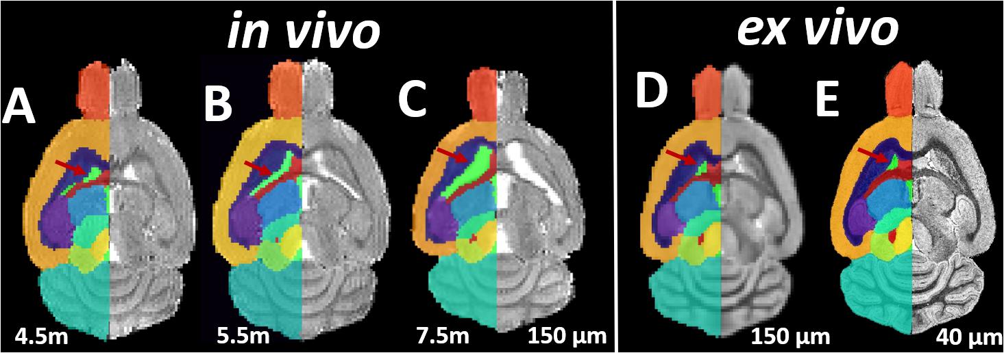
Figure 1. Representative axial slices of the Longitudinal in vivo and ex vivo images of the untreated transgenic mice, overlaid with the automatic parcellated structural labels. (A–C) In vivo images acquired at 4.5, 5.5, and 7.5 months. (D) The ex vivo image down-sampled to the same resolution of in vivo image (150 μm). (E) The ex vivo image with the original resolution (40 μm). Red Arrow: the longitudinal in vivo expansion and the ex vivo collapse of the ventricle is accurately delineated by parcellated labels.
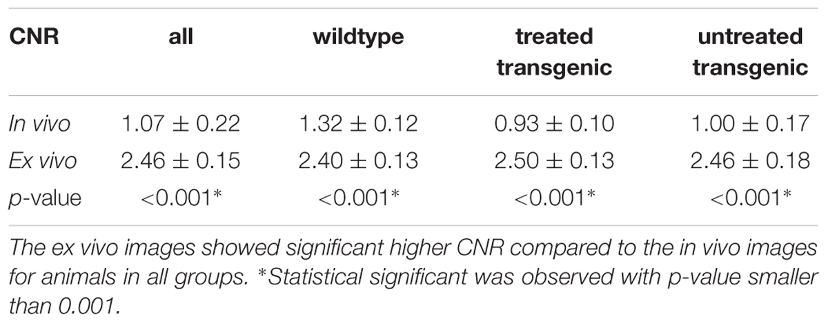
Table 1. Comparison of GM/WM tissue contrast-to-noise-ratio (CNR) between the in vivo and ex vivo images.
In vivo to ex vivo Volumetric Difference
Firstly, we compared the pair of in vivo and ex vivo structure volumes both acquired at 7.5 months. The ex vivo data were down-sampled to the same resolution as the in vivo data (150 um) to control the effect comes from the resolution difference. Figure 2 shows the results of the Bland–Altman analysis for the (Figure 2A) wild-type controls, (Figure 2B) the untreated rTg4510 group, and (Figure 2C) the doxycycline-treated rTg4510 group. The >100% relative volume shrinkage of the ventricles (Figure 2; red arrow) reflects the collapse of the ventricles from in vivo to ex vivo. The Bland–Altman plot shows variations in volume difference, indicating a non-linear non-uniform distribution of the volume shrinkage from in vivo to ex vivo.
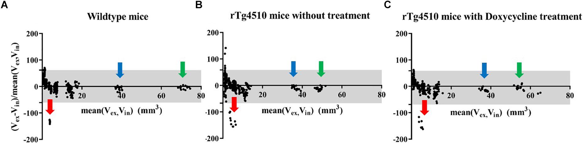
Figure 2. Bland–Altman plot showing the structure volume difference in the in vivo and ex vivo volume measurement (proportional to the mean volume of the two measurements). Gray area: 95% limit of agreement between in vivo and ex vivo measurements. (A) FVB/NCrl wild-type mice. (B) rTg4510 mice without treatment. (C) rTg4510 mice with doxycycline treatment. Arrows show examples of three distinctive structures, red arrow: ventricle; blue arrow: cerebellum; green arrow: neocortex.
We then plotted the percentage volume change as calculated from Bland–Altman analysis of all structure for each individual mouse in all three groups: the wild-type group, the untreated rTg4510 group, and the doxycycline-treated rTg4510 group (Figures 3A–C). The structures are listed in descending order of size: the top 29 structures are gray matter structures (except for the ventricles); the bottom 6 structures are white matter: (internal capsule, fimbria, and anterior commissure). We also performed paired t-test between the volume measured both in vivo and ex vivo for each group. The number at the right of each subplot represent the adjusted p-value of the paired t-test between the in vivo and ex vivo measurement (multiple comparisons were corrected with FDR = 0.05). Significant level of in/ex vivo differences are observed in most structures for all three groups, and the ventricular collapses are apparent for all groups (shown as the dark blue band), reflecting widespread changes induced by the preparation of the tissues for ex vivo scanning (Figures 3A–C). The ex vivo volumes were significantly smaller for the majority of the gray matter structures (e.g., neocortex, cerebellum, thalamus, olfactory bulb, hippocampus, caudate putamen, basal forebrain septum, hypothalamus, amygdala and superior/inferior colliculi) except for the central gray (the smallest labeled gray matter structure), which exhibited a significantly larger ex vivo volume compared to in vivo volume. On the other hand, most of the white structures demonstrated significantly larger ex vivo volumes than in vivo volumes (i.e., internal capsule, and fimbria) except for the smallest white matter structure, the anterior commissure, which was significantly smaller ex vivo. For the structure labeled “rest of midbrain” where there is a mix of white and gray matter, the volume change is not significant.
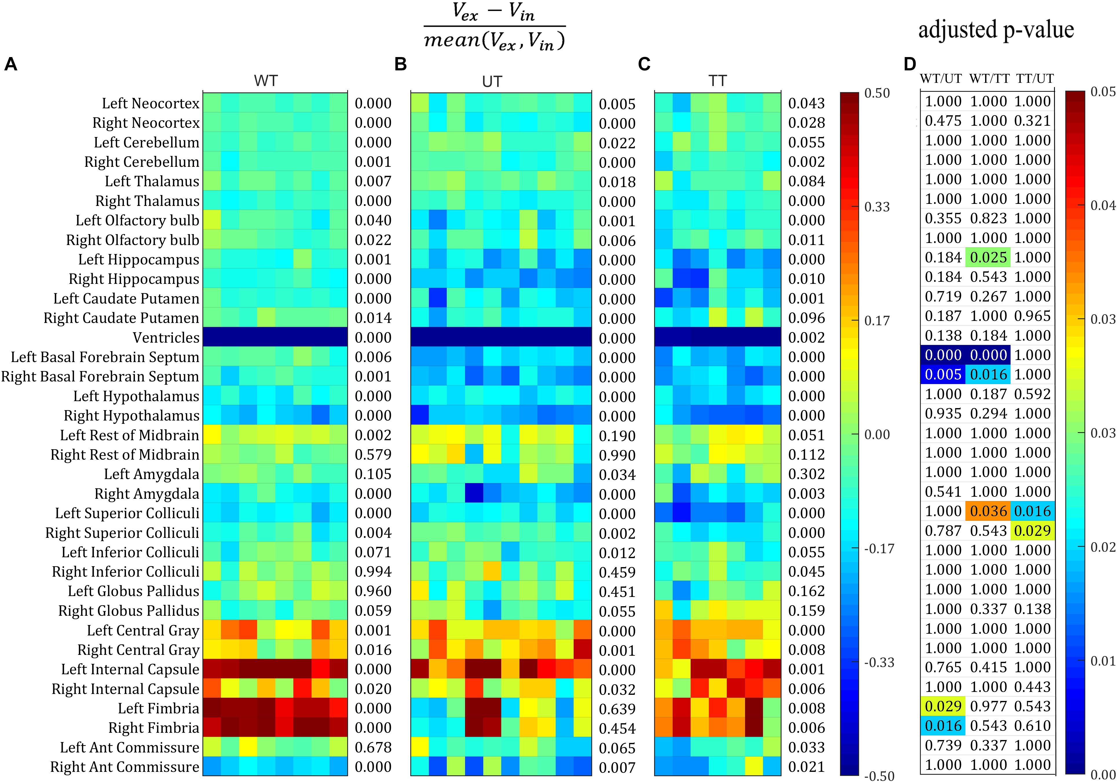
Figure 3. The percentage volume difference of each structure calculated from the Bland–Altman analysis for all the individual mouse across all three groups. Structures were listed from large to small top down. (A–C) The value were thresholded to within the range of [–0.5, 0.5]. The number at the right of each subplot represent the adjusted p-value of the paired t-test between the in vivo and ex vivo measurement (multiple comparisons were corrected with FDR = 0.05). (A) Wild-type group (WT). (B) Transgenic group without doxycycline treatment (untreated, UT). (C) Transgenic group with doxycycline treatment (treated, TT). (D) The adjusted p-value of the pairwise comparison among all three groups after ANOVA with Bonferroni post hoc test followed by multiple comparison corrections with FDR = 0.05. Only the significant p-values were shown with color (ranging from [0, 0.05]).
Figure 3D shows the statistical results of the ANOVA analysis, comparing the mean in/ex vivo volume difference among three groups (with Bonferroni post hoc test followed by multiple comparison corrections with FDR = 0.05). The majority of volume differences were not significantly different between groups; however, significant differences were detected for: the hippocampus (left side only) when comparing the wild-type controls to the treated rTg4510 group; the basal forebrain septum when comparing wild-type group to the rTg4510 groups (both the treated and untreated); the superior colliculi when comparing both the treated and untreated rTg4510 groups, as well as the wild-type to untreated rTg4510 group (left side only); and the fimbria when comparing between wild-type to the treated transgenic group (all shown in Figure 3D).
Group Difference Analysis
Next, we investigated whether the differences in in vivo and ex vivo volume measurements affected the statistical analysis when analyzing the treatment effect, by comparing the parcellated volumes of rTg4510 mice with and without doxycycline treatment. The structural volumes were normalized to TBV using the standardized residual (w-score), as described in the “Materials and Methods” section. Figure 4 shows the w-score of the volume for each structure across subjects for both rTg4510 groups (with untreated titled as UT, and treated group titled as TT), with the untreated group as the reference group. The w-score of each structure shows the difference between the normalized structure volume of the subject to the reference group mean, normalized by the reference group standard deviation. The number at the right of each subplot represents the adjusted p-value when comparing the untreated and treated group with two-tailed unpaired t-test. We performed the group difference analysis on both the single time-point data, as well as the longitudinal data, which are described in detail below.
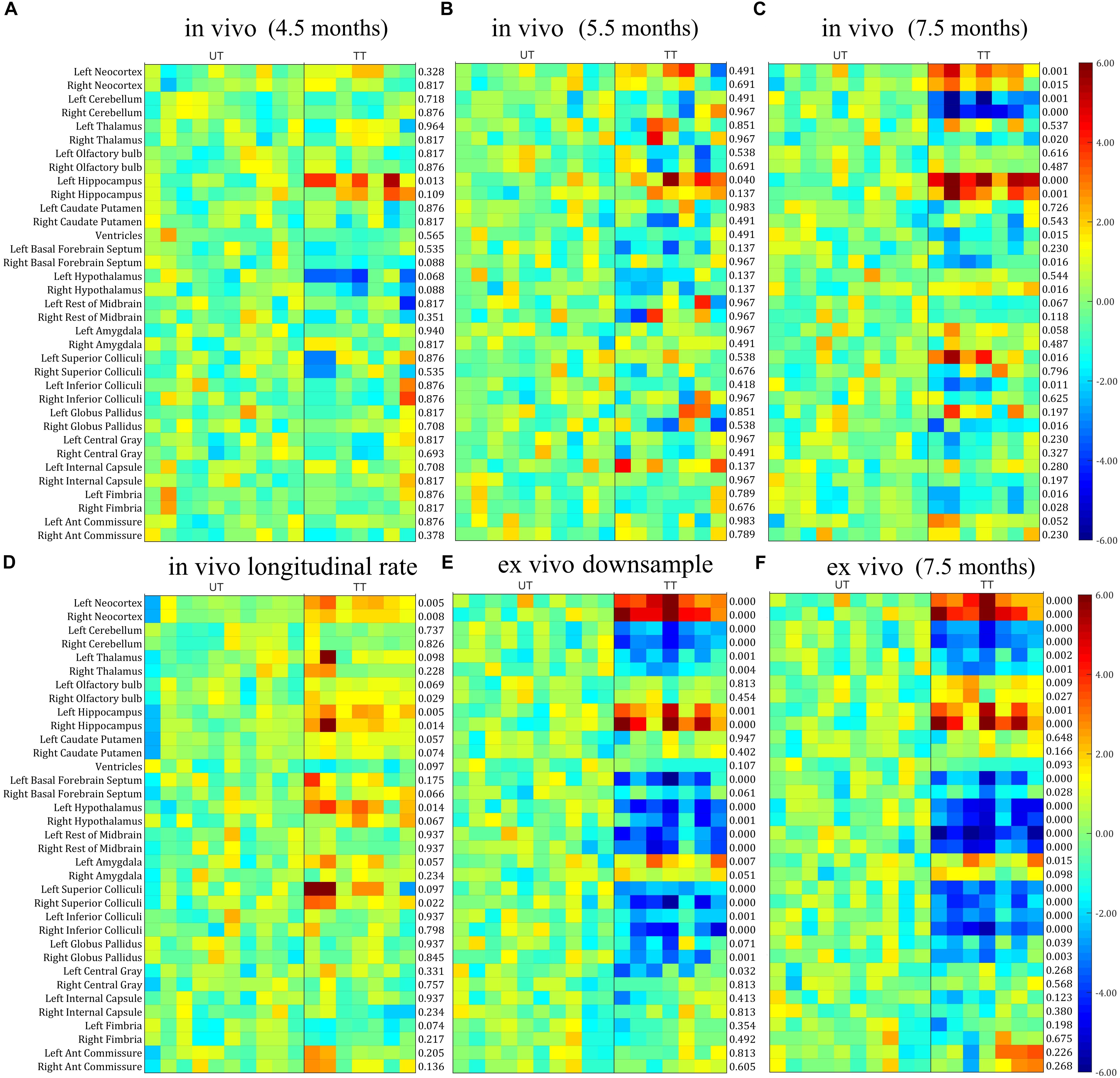
Figure 4. The w-score of the TBV normalized volume for each structure across subjects for both untreated (UT) and Doxycycline treated (TT) groups, with the untreated group as the reference group. The number at the right of each subplot represent the statistical results of unpaired two-tailed t-tests comparing the normalized structural volume of the treated and untreated group on both in vivo and ex vivo data. (A–C) In vivo data at different time-points (3.5, 5.5, and 7.5 months). (D) The longitudinal volume change calculated from the in vivo data at three time-points. (E) Ex vivo data down-sampled to the same resolution of the in vivo data (150 μm). (F) Original ex vivo data acquired at a resolution of 40 μm. All tests were corrected for multiple comparisons with a false discovery rate (FDR) of 0.05.
Single Time-Point Analysis
In order to make a direct comparison between structural changes identified in vivo versus ex vivo, we first compared the statistical analysis between in vivo and ex vivo data acquired at the same 7.5 months’ time-point. The in vivo results (Figure 4C) revealed a significant reduction in ventricle size after doxycycline treatment; however, this finding was not detected in the ex vivo data (Figure 4F) due to the ventricular collapse during the preparation of the post-mortem tissues. For the white matter (Figure 4; bottom six rows of each subplot), no significant volume differences were detected in any of the ex vivo white matter regions (Figure 4F), but a significant volume decrease was detected in the fimbria in the in vivo data (Figure 4C).
Within the gray matter, the in vivo data (Figure 4C) showed significant volume increases in the neocortex and hippocampus, right hypothalamus, left superior colliculi, and significant volume decreases in the right thalamus, right basal forebrain septum, left inferior colliculi and right globus pallidus. The statistical analysis of the ex vivo volumetric data acquired at the same time (Figure 4F) showed a similar pattern of group differences. However, the ex vivo volume analysis revealed additional significant volume decreases in the left thalamus, the olfactory bulb, the left basal forebrain septum, hypothalamus, superior/inferior colliculi, central gray (for both the raw and down-sampled data), and a significant volume increase in the left amygdala, which was not shown in the in vivo volumetric data. Interestingly for the hypothalamus, the in vivo results revealed an increase in volume within the hypothalamus associated with doxycycline treatment, while the ex vivo data showed a volume decrease. These discrepancies highlight the potential confounding effects of post-mortem tissue processing on ex vivo structural volumes. In addition, both the in vivo (Figure 4C) and ex vivo data showed significant cerebellar volume shrinkage after the doxycycline treatment (the third and fourth row of each subplot).
The down-sampled ex vivo data showed a similar level of statistical significance compared to the high resolution data, with a marginal reduction of statistical differences for most of the structures (Figures 4E,F); however, the significance levels of volume changes for a few structures (e.g., the olfactory bulb and the anterior commissure) were altered in the down-sampled data. For the olfactory bulb, the significant difference between treated and untreated rTg4510 groups did not persist after down-sampling, while for the anterior commissure, although no significant difference was detected for both cases, the adjust p-value became larger in the down-sampled data, indicating a reduction of statistical power after down-sampling. The fact that even the down-sampled data showed an improved level of significance relative to the in vivo analysis indicates that, the improved statistical power in the ex vivo data is not solely dominated by the improved resolution (40 um ex vivo versus 150 um in vivo), but other factors, such as improved CNR.
Longitudinal Analysis
When comparing the data from different time points from the in vivo data (Figures 4A–C), a pattern of increasing volumetric changes can be observed. Figure 4D shows the w-score and the statistical results of a two-tailed unpaired t-test (the adjusted p-value shown at the right of the plot) for the longitudinal unnormalized structural volume change rate, calculated from the in vivo data, which showed complementary information compared to the single timepoint volume difference (Figures 4A–C). Again, the untreated group is used as the reference group similar to the single-time-point analysis, so the higher values in the treatment subgroup represent better volume preserving effects comparing to the untreated subgroup, therefore reflecting the treatment effect. Significant differences in volume change rate were found in the neocortex, hippocampus, right olfactory bulb, and hypothalamus between the treated and untreated groups. In addition, the longitudinal data showed a higher level of significance of group difference for caudate putamen than the ex vivo data (and higher than the in vivo data for the right caudate putamen). These differences indicate complementary information over single timepoint in vivo and ex vivo volumetric analysis.
Comparison of Multivariate Classification Power
The results comparing the classification power of the in vivo and ex vivo data to correctly classify the untreated and treated group of mice using SVM with a linear kernel as the classifier are presented in Figure 5. Threefold cross-validation was performed, and the mean AUC of the ROC are presented as the classification performance, with a larger mean AUC representing better classification power. The in vivo data (Figure 5A) showed less classification power when compared with the ex vivo data, at either the original resolution (Figure 5B) or down-sampled to the same resolution as in vivo data (Figure 5E). In both scenarios, the ex vivo classification power showed all-correct prediction with AUC = 1; this can be attributed to the distinctive morphological differences between the two groups that was readily captured ex vivo. We noted that the classification power of both the in vivo single time-point volumetric analysis (Figure 5A) as well as the in vivo longitudinal rate of volumetric change across the three time-points (Figure 5C) demonstrated less classification power relative to the ex vivo data; however, the in vivo classification power showed marked improvements when these data (both the single time-point and the longitudinal) were combined (Figure 5D). This finding indicates that the two approaches for analysing the in vivo data capture complementary information, and the inclusion of both features can improve the classification performance. It is worth mentioning that, although we observed 100% accuracy (mean AUC = 1) for both the combined in vivo data (Figure 5D) as well as the two ex vivo analyses at original and down-sampled resolution (Figures 5B,E, respectively), this cannot be interpreted as the three set of data showing the same level of classification power.
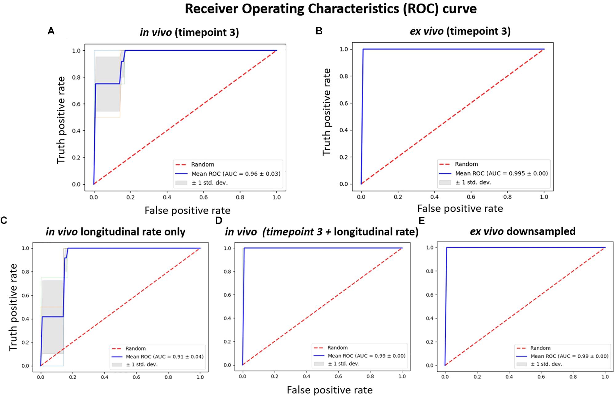
Figure 5. The receiver operating characteristics (ROC) of classification power for: (A) in vivo volume at timepoint 3 (7.5 months); (B) the corresponding ex vivo data with original resolution at timepoint 3 (7.5 months); (C) longitudinal in vivo volume change rate, calculated from the parcellation result of the data acquired at three timepoints (3.5, 5.5, and 7.5 months); (D) the in vivo feature combining both the single time point volume (at 7.5 months) and longitudinal volume change rate; (E) the ex vivo volume with volume down-sampled to the same resolution of the in vivo data. SVM with linear kernel is used as classifier, and the classification power is represented as the area under the curve (AUC) of the receiver operating characteristic (ROC) for threefold cross-validation.
The learning curve (Figure 6) shows the change of classification power to differentiate the doxycycline-treated and untreated rTg4510 groups using the SVM classifier, with respect to different sample size. The testing accuracies of both the in vivo and ex vivo data remained at 0.60 when the sample sizes were less than 10, and gradually improved with increasing sample sizes. The testing accuracy of ex vivo reached 1.00 when the sample size increased to 13 (Figure 6B), while the in vivo data with the same sample size only reached a testing accuracy of 0.86 (Figure 6A). For the down-sampled ex vivo data, the testing accuracy dropped slightly to 0.95 with a sample size of 13 (Figure 6E). Conversely, the testing accuracy of the longitudinal in vivo data increases from 0.60 to 0.90 when the sample size increases from 10 to 13 (Figure 6C). Finally, when the in vivo single time-point and longitudinal rate information were combined, the testing accuracy improved to 0.95 when sample size increases to 13; this is comparable to the down-sampled ex vivo data.
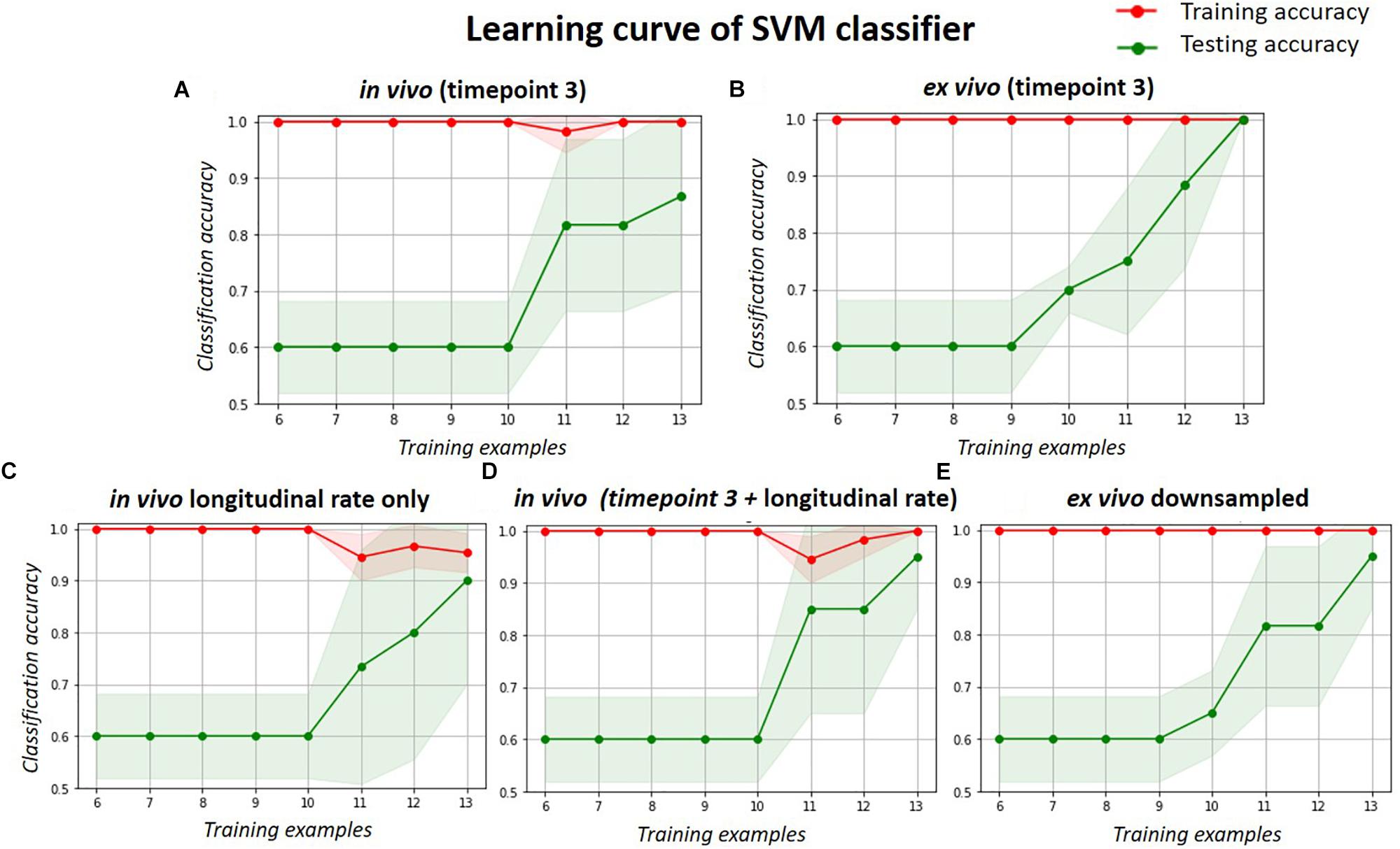
Figure 6. The learning curve of the SVM classifier with respect to different sample size, when classifying the treated and untreated group. Red lines represent the training accuracy, and the green lines represent the test accuracy. The shade region represents the standard deviation. Each subplot shows the classification accuracy for the: (A) in vivo data; (B) ex vivo data; (C) longitudinal in vivo data (in terms of volume change rate); (D) combination of the single timepoint cross-sectional and longitudinal in vivo data; and (E) ex vivo data down-sampled to the same resolution of in vivo data.
Evaluation of Individual Variation in the Longitudinal Scale
The longitudinal volume change of three structures most affected by AD: hippocampus, neocortex, and ventricle, were plotted in Figure 7, for all three experimental groups: wildtype, rTg4510 mice without treatment, and rTg4510 mice with doxycycline treatment. The longitudinal trend in the result clearly shows the continuous progression of pathologies (wildtype vs. untreated transgenic group), as well as the effect of doxycycline treatment (untreated vs. treated transgenic group) in all three structures. Statistical analysis indicated that the hippocampal/cortical atrophies start to manifest as early as 4.5 months, and the ventricle expansion starts from 5.5 months (as indicated by the significant volume difference between wildtype and untreated transgenic group). In addition, the treatment effect appeared as early as 4.5 months in the hippocampus, and is observable in neocortex and ventricles at 7.5 months (as indicated by the significant volume difference between the treated and untreated transgenic group). These results align with the reported longitudinal disease progression time windows in previously published studies and validate the timepoints selected in this study.
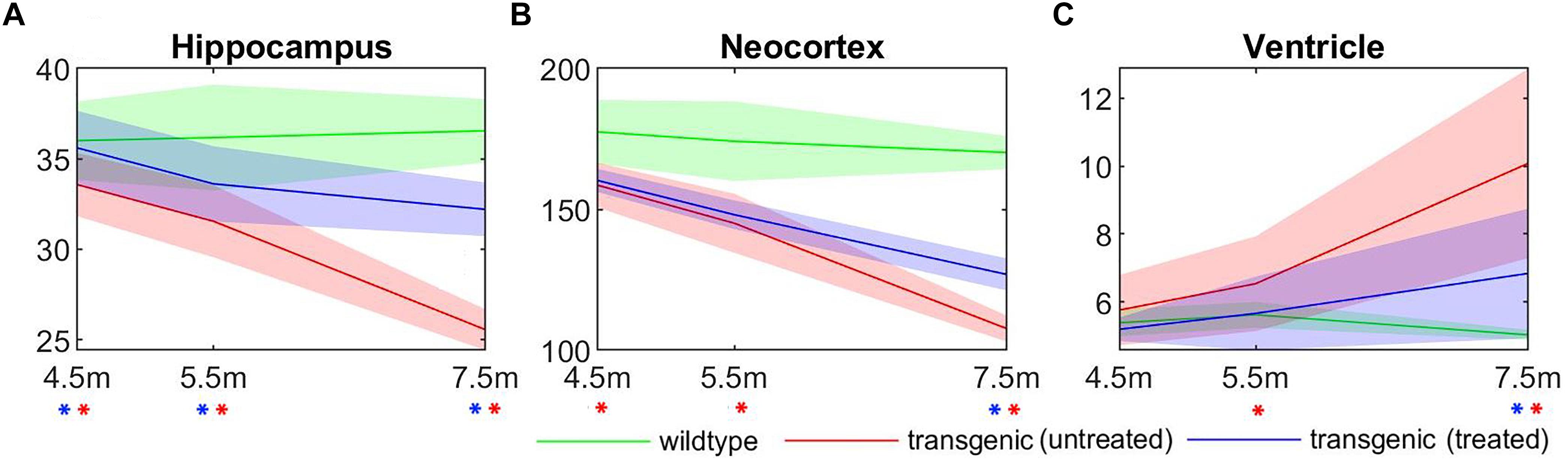
Figure 7. The longitudinal absolute structural volume change of (A) hippocampus, (B) neocortex, and (C) ventricle for all three experimental groups. Green: wild-type mice, red: transgenic mice without treatment, blue: transgenic mice with doxycycline treatment. ∗(red): significant volume difference was detected between untreated transgenic and wild-type mice; ∗(blue): significant volume difference was detected between treated and untreated transgenic mice. ANOVA with Bonferroni post hoc test followed by multiple comparison corrections with FDR = 0.05. Unit of the y-axis: mm3.
It can be observed from Figure 7 that, compared to the hippocampus and neocortex, the ventricles showed larger individual variation of disease pathology progression, especially in the later timepoints (5.5 and 7.5 months), and exhibit less significant group differences. Therefore, we further analyzed the longitudinal individual variation in the in vivo data using LME model. Table 2 shows the result comparing different LEM model performance when evaluating the individual variations in the in vivo data. Models performances were evaluated with AIC, and the statistical difference between the corresponding REML estimations. Comparing to the fixed-effect model, the random intercept model performance improves for all three AD-related structures, indicating significant individual variation in the structural volume measurements. The random intercept and slope model showed further performance improvement, demonstrating additional individual variation in the longitudinal volume change rate.
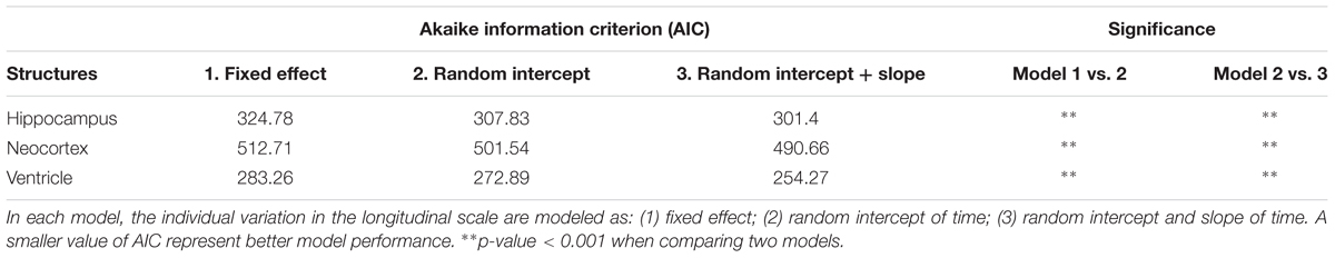
Table 2. Comparison of different linear mixed effect (LME) models in terms of AIC and significant difference in REML estimation.
Figure 8 shows the comparison of the individual percentage residual of the volumes for all three structures across all three group at different timepoints. The random intercept model (Figure 8B) showed smaller relative residual compared to the fixed-effect model (Figure 8A), while the random intercept and slope model (Figure 8C) reduced the relative residual further, which agree with the model comparison results shown in Table 2. In the fixed-effect model (Figure 8A), the individual variation in the neocortex (middle row) is the smallest among the three structures across all three timepoints, indicating small individual variation in the cortical region. In addition, with the fixed effect model and the random intercept model (Figures 8A,B), the ventricle (bottom row) exhibits larger relative residual compared to hippocampus and neocortex for both the untreated and treated transgenic group (as shown in red and blue box), especially in the later timepoints (5.5 and 7.5 months). This result confirms the larger individual variation in the ventricles in the longitudinal scale. The relative residual is greatly reduced after the individual variance is controlled by including the random effects to the slope of time in the model (Figure 8C, bottom row).
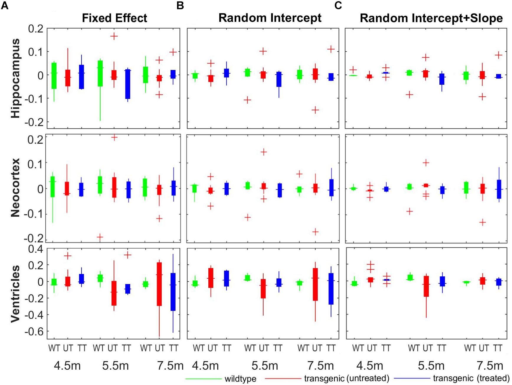
Figure 8. The comparison of the model fitting between the three linear mixed-effect (LME) models. (A) Fixed-effect model, in which individual variation was not modeled explicitly, and the longitudinal measurements for each individual subject are modeled as fixed-term; (B) random intercept model, in which individual variance on the absolute volume was explicitly modeled by introducing a random-effect term on the intercept; (C) random intercept and slope model, in which the individual variance on the longitudinal scale was also modeled by adding an additional random-effect term over the slope of time. The y-axis represent the relative residual which is the ratio between the model residual and the actual measured volume (unit: percentage).
Discussion
When designing experiments to study diseases using mouse models, one must choose whether to scan animals in vivo or ex vivo. It is sometimes a controversial choice as each of these imaging paradigms has its own strengths and weaknesses. In this study, we investigated both the progression of longitudinal structural volume changes, as well as the in vivo to ex vivo volumetric changes due to the preparation of post-mortem tissues. We demonstrated how this choice of paradigm will affect volumetric analysis using automated brain structural parcellation, both in terms of group difference analysis, as well as classification power.
In vivo to ex vivo Volumetric Change
Previous studies exploring volumetric changes from in vivo to ex vivo have shown controversial conclusions. Early histology studies have shown that both perfusion and fixation processes cause tissue shrinkage (Palay et al., 1962; Cragg, 1980). With MRI data, Schulz et al. (2011) investigated the effect of fixation on the volume of the human brain for up to 70 days using image registration, and found unevenly distributed brain shrinkage after initial expansion. Conversely, a study by Kotrotsou et al. (2014) found a linear correlation between ex vivo and in vivo gray matter volumes, with no significant change during the 6 months’ fixation period. Studies on preclinical imaging data also show inconsistent results. Zhang et al. (2010) used manual segmentation and showed a decrease in ex vivo brain volume (4.47% for wild-type mice, and 8% for Huntington’s disease mice). Meanwhile, Ma et al. (2005, 2008) used semi-automatic segmentation propagation and found a 10.6% shrinkage in ex vivo brain volumes relative to in vivo brain volumes, and reported that some parts of the gray matter shrunk from in vivo to ex vivo whilst others expanded. However, the in vivo and ex vivo imaging datasets in these studies were acquired from different mice populations (of the same strain), and the ex vivo specimens were scanned after physical skull removal, with brain tissue loss notable from the images. On the other hand, Oguz et al. (2013) performed single-atlas segmentation-propagation on rat brains (male Wistar) but found no significant change between the in vivo and ex vivo datasets for TBV, and structural volumes. Recent work by Holmes et al. (2017) reported a reduction in the TBV of 10.3% between in vivo and ex vivo mouse brain MRI and non-uniform morphological change using tensor based morphometry (TBM). Such variance in these different volumetric studies could be attributed to factors such as animal strain difference, pathological model diversity and protocol variation of post-mortem tissue processing. Consequently, these various factors might impact the accuracy and reliability of quantitative measurements extracted from ex vivo data.
Our result confirmed the uneven distribution of volumetric changes across different brain structures, as published studies have reported (Ma et al., 2005, 2008; Zhang et al., 2010; Schulz et al., 2011; Holmes et al., 2017). Our study expanded upon these previous findings by quantifying the volume change for each individual structure, in both the gray and white matter. We demonstrated that the post-mortem fixation and perfusion processes introduce different morphological alterations that affects different tissue types: after the ex vivo tissue processing, the majority of gray matter structures shrink, while most white matter structures expand. Furthermore, the collapse of almost the entire ventricular space results in a dramatic reduction in CSF volume ex vivo. These observed changes in gray and white matter volumes were non-uniformly distributed within each tissue types. Furthermore, our results showed differences in the level of volumetric changes across the three groups of mice: the doxycycline-treated rTg4510s, untreated rTg4510s and wild-type controls. Such variation in volume changes among ex vivo tissue types, tissue structures, and between groups, will obviously complicate the interpretation of morphological analysis using techniques such as voxel-based morphometry, which relies on the estimation of proportional volume change between gray matter and white matter. Therefore, although the ex vivo volumetric analysis in this study demonstrated superior statistical and classification power for group difference analysis compared to the in vivo data acquired at the same time-point, it is, however, difficult to differentiate the proportion of such improvements which represent the true biological effect, and the changes that manifest as a result of the post-mortem tissue processing. For example, the level of in/ex vivo volume difference of the superior colliculi is significantly higher in the doxycycline treated group than the untreated group, as shown in Figure 3D. Therefore, the increased ex vivo statistical power of the group difference detected within the superior colliculi (as shown in Figures 4C,E) is, in fact, a combination of actual biological morphological differences, and effects originating from the ex vivo tissue processing.
Specifically, ventricular expansion is an important neuroimaging biomarker for neurodegenerative diseases such as AD (Nestor et al., 2008; Weiner, 2008). For the ex vivo ventricular measurements, the ventricle collapse and the loss of ventricular CSF in the post-mortem brain tissue preservation process. Our study reported a large ventricles volumetric loss from in vivo to ex vivo which aligns with previous studies: (Ma et al., 2008; Zhang et al., 2010).
The white matter expansion is also interesting, which indicates potential microstructural-level volume expansion of the white matter tract. Compared to the GM, the WM contains significantly less water (∼70% vs. ∼85%) and more lipid (16–22/100 g vs. 5–6/100 g) (Davison and Wajda, 1962). The post-mortem brain tissue fixation changes various MR indexes significantly, such as T1, the magnetization transfer ratio (MTR), and the macromolecular protons fraction, which also differs between GM and WM (Schmierer et al., 2008, 2010). Such compositional and signal difference will obviously affect the volume change to different tissues types. Von Halbach und Bohlen et al. (2014) proposed an alternative method to conduct post-mortem ex vivo imaging directly after the animal has been sacrificed, to prevent the potential volume changes associated with the preparation of fixed tissues. However, such ex vivo imaging procedure is inevitably contaminated by the fast post-mortem tissue degradation (Sun et al., 2015). This becomes even more significant given the long scanning time of the ex vivo imaging which easily adds up to several hours. In addition, tissue samples frequently undergo histological evaluation after ex vivo imaging to corroborate structural changes with alterations occurring at the cellular level. The advanced brain tissue decomposition after long scans will also affect the quality of the histology evaluation (Von Halbach und Bohlen et al., 2014).
It is worth noting that, the measurements for the ex vivo images depend highly on the post-mortem tissue processing protocol in MR microscopy, In the case of this study, the in-skull brain tissue was soaked in contrast-enhanced agent for 9 weeks before ex vivo imaging, which would theoretically aggravate the tissue dehydration. The protocol diversity among various ex vivo studies should account for a large portion of the difference in the corresponding results. Therefore, the ex vivo brain structure volume change reported in the current paper should be regarded as specific to the active staining tissue processing protocol used in this study. On the other hand, such variation in the results of different ex vivo studies emphasize the importance and advantage of protocol consistency for in vivo measurements.
Comparison Between in vivo and ex vivo Morphological Analysis
Lerch et al. (2012) have compared the theoretical statistical power between in vivo and ex vivo imaging, using a pre-determined variance value with simulated deformation on the hippocampus. Their result showed that ex vivo imaging provides better precision and should be preferred if the volume is normalized to TBV, as the normalization process regress out the effect of gross brain volume difference between individual animals; while in vivo measurements give better results on absolute volume measurements and can provide more accuracy in longitudinal studies than cross-sectional ex vivo measurements. In a recent study, Holmes et al. (2017) have conducted power analysis to determine the required sample size in order to detect a specific amount of local morphological variation either in vivo or ex vivo. Careful power analysis is important to determine the appropriate sample size given effect size. Comparing with voxel-wise statistical analysis such as TBM (Holmes et al., 2017), the required sample size to detect volume difference is smaller for structural-based analysis, as the effect toward all the voxels in each structure are grouped together if the intra-structural volume change is homogenous enough. Our findings extended these theoretical analyses with application to longitudinal in vivo analysis on each individual structural volume. Although the longitudinal analysis based on structure volume change rate by itself is less powerful to statistically compare and classify different groups, it indeed showed complementary information over the single-time-point volume information. We showed that by combining the both the longitudinal and cross-sectional in vivo volumetric information, there is an improvement of the classification power.
In this study, we modeled the longitudinal volume change as a liner effect for each all structures. However, the change of ratio might be in fact not linear, and the time that volume change occurs can be different for different structures (either due to the nature of the pathological process, or the treatment start to show effect). Therefore, a model alternative to the linear regression would potentially represent the actual volume change better and further improved the in vivo analysis results. Furthermore, by integrating the volume information with other in vivo assessment to form multimodality analysis (such as CEST and CBF (Wells et al., 2015; Holmes et al., 2017) could potentially further improve the statistical and classification power for the in vivo data.
Specifically, it is interesting that both the in vivo and ex vivo data of the transgenic mouse at 7.5 months showed cerebellar shrinkage after doxycycline treatment. The cerebellum is traditionally considered unaffected in AD, although recent studies have shown increase evidence that it is also affected during the AD disease progression (Larner, 1997; Jacobs et al., 2018), which is also the case for rTg4510 (Xie et al., 2010). However, further investigations are required to draw connection between potential neuroprotective or neurotoxicity effect of doxycycline to the cerebellum, such as the cerebellar plasticity (Ito, 2012), to help us understand the observation reported in this study.
In this study, we used the w-score (Eq. 3, Figure 4) to visualize the group difference rather than the raw volume. The advantage of using w-score is that the volume measurements of each individual structure are transformed to the reference group mean and normalized by the reference group standard deviation. This process standardizes the group difference for all the features to the same scale, effectively improve the feature-based classification (Fortin et al., 2017; Rozycki et al., 2017).
In experiments with biological tissues or subjects, the variations of the individual measurements are often observed. The presence of outliers may affect the power of statistical analysis, especially in cases where the sample number is relatively small This is a common issue that animal studies usually suffer from, especially when the effect size of the group difference is small. In this study, we presented a data visualization method that is capable of pooling the entire dataset within a panorama figure showing multiple measurements for each individual (as shown in Figures 3, 4). Moreover, presenting the w-score of the raw measurement ensures meaningful visualization of the individual variation while preserving the statistical analysis results, since all the data are shifted and scaled by the same number (i.e., the mean and standard deviation of the reference group). Such data visualization technique is an intuitive way to demonstrate internal data inhomogeneity on very large databases (Ma et al., 2018), and in this study, showed individual variations in small dataset as well. In addition, comparison of different LME models demonstrated region-specific, group-dependent, and time-variate individual variations in the longitudinal in vivo measurement of structure volume.
When classifying the treated and untreated group, the SVM showed satisfactory results even with the relatively small sample size (Figures 5, 6), thanks to the relatively large effect size between the two groups. Never the less, the classification power analysis result clearly demonstrated the improvement in testing accuracy after combining cross-sectional and longitudinal in vivo data when comparing with ex vivo data, although larger sample size is required to reduce the testing error when the effect size between the groups is small (Figueroa et al., 2012; Beleites et al., 2013). Techniques such as bootstrap aggregating (a.k.a bagging) can be used, along with increasing the number of data, to reduce the variance in the training, improve the classification accuracy, and avoid overfitting (Dietterich, 2000).
In the field of preclinical imaging research, we anticipate that the widely regarded ‘gold standard’ for investigating mouse models at the macroscopic level to shift from histology to ex vivo imaging, and later to in vivo imaging. Such a shift in the imaging paradigm will not only enable the longitudinal assessment of neuroanatomical changes but will also help reduce the number of animals dedicated to preclinical studies (Gunn et al., 2012; Home Office, 2014).
Limitations of the Current Study
In the current study, we used TBV as a normalization term. However, the TBV itself is a dependent variable toward the treatment effect (Holmes et al., 2017). A better alternative to normalized the data should be estimating the total intracranial volume (TIV) employing tissue classification techniques, which use expectation maximization to estimate the tissue probability for each voxel, including gray matter, white matter, CSF, and non-brain tissues, and estimate the TIV as the summation of all types of brain tissues (Lemieux et al., 2003; Acer et al., 2007; Ridgway et al., 2011). However, a tissue probability map is necessary as prior information to initialize the expectation-maximization procedure. One of the current limitations in mouse brain MRI studies is the lack of such accurate tissue probability map. A tissue classification framework with accurate tissue probability maps (Sawiak et al., 2013; Powell et al., 2016; Hikishima et al., 2017) would be beneficial for future preclinical studies.
In the section of classification power comparison, no feature selection and hyperparameter tuning were performed, and the selected models and hyperparameters do not necessarily reflect the optimal choice or value for the group classification for the current dataset. However, model optimization is not the focus of this study, and the main purpose of this section of analysis is to compare the classification performance using the same model and parameter when applied from the dataset collected from the same sample but with different measurement (in vivo versus ex vivo).
Furthermore, in the current study, the in vivo and ex vivo images were acquired using different imaging protocols with different scanning sequences and coils, for comparing the best quality of each. Consequently, the measured in/ex vivo volume difference is a combination of the biological/pathological change and the measurement difference due to different image quality (e.g., CNR) between the in vivo and ex vivo images. In an ideal experiment setup, the same scanning protocol (i.e., the same coil and scanning sequence) would be used to acquire both in vivo and ex vivo images in order to have a bias-free comparison to assess the volume change accurately. This will on one hand effectively eliminate some confounding factors from the images, but on the other hand, losing its representation of the best image quality acquired in real practice. One effort to alleviate such bias in this study is to down-sample the ex vivo data to the same resolution of the in vivo data, which reduces the bias that comes directly from the resolution difference. On the other hand, even with the similar resolution, the higher GM/WM CNR in the ex vivo data, as shown in Table 1, helps to improve the automatic structural parcellation accuracy, and demonstrated higher statistical and classification power.
In this study, only female mice are used to control the effect of sex toward the variation of the data. However, sex-specific differences have been reported in AD (Mielke et al., 2014; Mazure and Swendsen, 2016; Laws et al., 2018), such as faster cognitive decline and pathological progression in female than male (Ferretti et al., 2018). Specifically, the rTg4510 mice model also showed significantly higher levels of Tau-induced pathology in female mice at 5.5 months (Yue et al., 2011). Therefore, the result and conclusion presented in this study can only be referred to females, and data from both sexes are required to draw more generous conclusions about the disease specification and potential treatment effect for precision medicine.
Finally, the variation comes from scanning gradient coil difference can be alleviated through careful gradient calibration. Gradient calibration is crucial for MRI to eliminate any time-dependent gradient shift to ensure the acquired image represented the tissue volumes accurately. This is especially important for longitudinal studies across a long period of time, as well as the comparison between images acquired with different gradient coil, as in the case of our study. However, unlike clinical systems, the frequency of gradient calibration for the preclinical system is sometimes insufficient. By employing the gradient calibration protocol we developed previously and employed in this study (O’Callaghan et al., 2014), we detected that the 72 mm birdcage radiofrequency (RF) coil we used for in vivo scan comes with around 0.1% gradient shift per month, which will cause significant system bias for both longitudinal analysis using in vivo data, as well as analysis comparing in vivo and ex vivo data acquired from different gradient coil. The effect of such longitudinal imaging gradients shift has been alleviated through proper gradient calibration, and the associated biases have been removed prior to any longitudinal and cross-sectional analysis.
Conclusion
In conclusion, in this paper, we presented our study to compare the volumetric analysis for longitudinal in vivo imaging and cross-sectional ex vivo imaging using automated mouse brain MRI structural parcellation. We showed non-uniformly distributed structural volume changes from in vivo to ex vivo measurements across different tissue types. We also demonstrated the effect of mouse strains and drug treatment toward the in vivo to ex vivo volume change. Our result demonstrated higher statistical and classification power using the ex vivo structure volume compared to the in vivo counterpart, although the volume differences in the ex vivo data represent a combination of both the biological/physiological effect as well as the effect due to post-mortem tissue processing. On the other hand, the in vivo measurements identified ventricular shrinkage, while ex vivo measurements were not sensitive to these changes due to the ventricular collapse during the preparation of the post-mortem tissues. In addition, we showed that the longitudinal in vivo imaging provided complementary information other than single-timepoint measurement. Incorporating the information obtained from the longitudinal data as additional features significantly improves the classification power.
Ethics Statement
All studies were carried out in accordance with the recommendations of United Kingdom’s Animals (Scientific Procedures) Act of 1986 and approved by the UCL internal ethics committee.
Author Contributions
ML, SO, MM, and MC contributed to the conception and design of the study, provide infrastructure, and provide overall supervision. RJ, MO, and EC designed and advised on the animal experiment design and treatment experiment design. HH performed the data acquisition experiments, optimize the protocol, and acquired the data. OI manages the experimental setup as well as the treatment procedure. DM, NP, and JO performed the first phase of data processing and analysis. DM, MB, and KP contributed and performed the second batch of the data analysis and visualization. DM wrote the first draft of the manuscript. HH, IH, and NP refined the experimental setup and data analysis protocol. All authors contributed to the manuscript revision, read and approved the submitted version.
Funding
This work was carried out in collaboration with, and part funded by, Eli Lilly and Company. DM received a proportion of funding from UCL Faculty of Engineering funding scheme, and a proportional of funding from Alzheimer Society of Canada through the Alzheimer Society Research Program (ASRP). HH was supported by an NC3Rs studentship (NC/K500276/1). JO was supported by the UK Medical Research Council Doctoral Training Grant Studentship (MR/J500422/1). MC received funding from EPSRC (EP/H046410/1). MM was supported by the UCL Leonard Wolfson Experimental Neurology Centre (PR/ylr/18575). NP was supported by the UK Medical Research Council Doctoral Training Grant Studentship (MR/G0900207-3/1). SO received funding from the EPSRC (EP/H046410/1, EP/J020990/1, and EP/K005278), the MRC (MR/J01107X/1), the EU-FP7 project VPH-DARE@IT (FP7-ICT-2011-9-601055), the NIHR Biomedical Research Unit (Dementia) at UCL, and the National Institute for Health Research University College London Hospitals Biomedical Research Centre (NIHR BRC UCLH/UCL High Impact Initiative – BW.mn.BRC10269). ML received funding from the Medical Research Council (MR/J013110/1), the UK Regenerative Medicine Platform Safety Hub (MRC: MR/K026739/1) (IRIS 104393) and the King’s College London and UCL Comprehensive Cancer Imaging Centre CR-UK & EPSRC (000012287) in association with the MRC and DoH (United Kingdom). KP and MB were funded by the Natural Sciences and Engineering Research Council of Canada (NSERC), Canadian Institutes of Health Research (CIHR), Brain Canada, Pacific Alzheimer’s Research Foundation, the Michael Smith Foundation for Health Research (MSFHR), and the National Institute on Aging (R01 AG055121-01A1).
Conflict of Interest Statement
The authors declare that the research was conducted in the absence of any commercial or financial relationships that could be construed as a potential conflict of interest.
References
Acer, N., Sahin, B., Baş, O., Ertekin, T., and Usanmaz, M. (2007). Comparison of three methods for the estimation of total intracranial volume: stereologic, planimetric, and anthropometric approaches. Ann. Plast. Surg. 58, 48–53. doi: 10.1097/01.sap.0000250653.77090.97
Aljabar, P., Heckemann, R. A., Hammers, A., Hajnal, J.V. V., and Rueckert, D., (2007). “Classifier selection strategies for label fusion using large atlas databases,” in Proceddings of MICCAI: International Conference on Medical Image Computing and Computer-Assisted Intervention, MICCAI’07 (Berlin: Springer-Verlag), 523–531. doi: 10.1007/978-3-540-75757-3_64
Almhdie-Imjabber, A., Léger, C., Lédée, R., and Harba, R. (2010). Atlas-assisted segmentation of cerebral structures of mice. IWSSIP 2010, 3–6.
Altman, D. G., and Bland, J. M. (1983). Measurement in medicine: the analysis of method comparison studies. J. R. Stat. Soc. Ser. D (Stat.) 32, 307–317. doi: 10.2307/2987937
Bai, J., Trinh, T. L. H., Chuang, K.-H., and Qiu, A. (2012). Atlas-based automatic mouse brain image segmentation revisited: model complexity vs. image registration. Magn. Reson. Imaging 30, 789–798. doi: 10.1016/j.mri.2012.02.010
Beleites, C., Neugebauer, U., Bocklitz, T., Krafft, C., and Popp, J. (2013). Sample size planning for classification models. Anal. Chim. Acta 760, 25–33. doi: 10.1016/j.aca.2012.11.007
Calmon, G., and Roberts, N. (2000). Automatic measurement of changes in brain volume on consecutive 3D MR images by segmentation propagation. Magn. Reson. Imaging 18, 439–453. doi: 10.1016/S0730-725X(99)00118-6
Cardoso, M. J., Leung, K., Modat, M., Keihaninejad, S., Cash, D., Barnes, J., et al. (2013). STEPS: similarity and truth estimation for propagated segmentations and its application to hippocampal segmentation and brain parcelation. Med. Image Anal. 17, 671–684. doi: 10.1016/j.media.2013.02.006
Chumbley, J. R., and Friston, K. J. (2009). False discovery rate revisited: FDR and topological inference using Gaussian random fields. Neuroimage 44, 62–70. doi: 10.1016/j.neuroimage.2008.05.021
Cleary, J. O., Wiseman, F. K., Norris, F. C., Price, A. N., Choy, M., Tybulewicz, V. L. J., et al. (2011). Structural correlates of active-staining following magnetic resonance microscopy in the mouse brain. Neuroimage 56, 974–983. doi: 10.1016/j.neuroimage.2011.01.082
Collij, L. E., Heeman, F., Kuijer, J. P. A., Ossenkoppele, R., Benedictus, M. R., Möller, C., et al. (2016). Application of machine learning to arterial spin labeling in mild cognitive impairment and alzheimer disease. Radiology 281, 865–875. doi: 10.1148/radiol.2016152703
Cragg, B. (1980). Preservation of extracellular space during fixation of the brain for electron microscopy. Tissue Cell 12, 63–72. doi: 10.1016/0040-8166(80)90052-X
Crum, W. R., Hartkens, T., and Hill, D. L. G. (2004). Non-rigid image registration: theory and practice. Br. J. Radiol. 77, S140–153. doi: 10.1259/bjr/25329214
Davison, A. N., and Wajda, M. (1962). Analysis of lipids from fresh and preserved adult human brains. Biochem. J. 82:113. doi: 10.1042/bj0820113
Dietterich, T. G. (2000). An experimental comparison of three methods for constructing ensembles of decision trees: bagging, boosting, and randomization. Mach. Learn. 40, 139–157. doi: 10.1023/A:1007607513941
Ferretti, M. T., Iulita, M. F., Cavedo, E., Chiesa, P. A., Schumacher Dimech, A., Santuccione Chadha, A., et al. (2018). Sex differences in Alzheimer disease — the gateway to precision medicine. Nat. Rev. Neurol. 14, 457–469. doi: 10.1038/s41582-018-0032-9
Figueroa, R. L., Zeng-Treitler, Q., Kandula, S., and Ngo, L. H. (2012). Predicting sample size required for classification performance. BMC Med. Inform. Decis. Mak. 12:8. doi: 10.1186/1472-6947-12-8
Fortin, J.-P., Parker, D., Tunç, B., Watanabe, T., Elliott, M. A., Ruparel, K., et al. (2017). Harmonization of multi-site diffusion tensor imaging data. Neuroimage 161, 149–170. doi: 10.1016/j.neuroimage.2017.08.047
Gunn, M., Vaudano, E., and Goldman, M. (2012). The rational use of animals in drug development: contribution of the innovative medicines initiative. Altern. Lab. Anim. 40, 307–312.
Hikishima, K., Komaki, Y., Seki, F., Ohnishi, Y., Okano, H. J., and Okano, H. (2017). In vivo microscopic voxel-based morphometry with a brain template to characterize strainspecific structures in the mouse brain. Sci. Rep. 7:85. doi: 10.1038/s41598-017-00148-1
Holmes, H. E., Colgan, N., Ismail, O., Ma, D., Powell, N. M., O’Callaghan, J. M., et al. (2016). Imaging the accumulation and suppression of tau pathology using multiparametric MRI. Neurobiol. Aging 39, 184–194. doi: 10.1016/j.neurobiolaging.2015.12.001
Holmes, H. E., Powell, N. M., Ma, D., Ismail, O., Harrison, I. F., Wells, J. A., et al. (2017). Comparison of in vivo and ex vivo MRI for the detection of structural abnormalities in a mouse model of tauopathy. Front. Neuroinform. 11:20. doi: 10.3389/fninf.2017.00020
Home Office (2014). Guidance on the Operation of the Animals (Scientific Procedures) Act 1986. Available at: https://www.gov.uk/guidance/guidance-on-the-operation-of-the-animals-scientific-procedures-act-1986
Jacobs, H. I. L., Hopkins, D. A., Mayrhofer, H. C., Bruner, E., Van Leeuwen, F. W., Raaijmakers, W., et al. (2018). The cerebellum in Alzheimer’s disease: evaluating its role in cognitive decline. Brain 41, 37–47. doi: 10.1093/brain/awx194
Kim, Y., and Kong, L. (2016). Improving classification accuracy by combining longitudinal biomarker measurements subject to detection limits. Stat. Biopharm. Res. 8, 171–178. doi: 10.1080/19466315.2016.1142889
Klingenberg, C. P. (1996). Individual variation of ontogenies: a longitudinal study of growth and timing. Evolution (N. Y.) 50, 2412–2428. doi: 10.1111/j.1558-5646.1996.tb03628.x
Kotrotsou, A., Bennett, D. A., Schneider, J. A., Dawe, R. J., Golak, T., Leurgans, S. E., et al. (2014). Ex vivo MR volumetry of human brain hemispheres. Magn. Reson. Med. 71, 364–374. doi: 10.1002/mrm.24661
La Joie, R., Perrotin, A., Barre, L., Hommet, C., Mezenge, F., Ibazizene, M., et al. (2012). Region-specific hierarchy between atrophy, hypometabolism, and -amyloid (a) load in Alzheimer’s disease dementia. J. Neurosci. 32, 16265–16273. doi: 10.1523/JNEUROSCI.2170-12.2012
Larner, A. J. (1997). The cerebellum in Alzheimer’s disease. Dement. Geriatr. Cogn. Disord. 8, 203–209. doi: 10.1159/000106632
Lavenex, P., Lavenex, P. B., Bennett, J. L., and Amaral, D. G. (2009). Postmortem changes in the neuroanatomical characteristics of the primate brain: hippocampal formation. J. Comp. Neurol. 512, 27–51. doi: 10.1002/cne.21906
Laws, K. R., Irvine, K., and Gale, T. M. (2018). Sex differences in Alzheimer’s disease. Curr. Opin. Psychiatry 31, 133–139. doi: 10.1097/YCO.0000000000000401
Lee, H., Nakamura, K., Narayanan, S., Brown, R. A., and Arnold, D. L. (2018). Estimating and accounting for the effect of MRI scanner changes on longitudinal whole-brain volume change measurements. Neuroimage 184, 555–565. doi: 10.1016/J.NEUROIMAGE.2018.09.062
Lemieux, L., Hammers, A., Mackinnon, T., and Liu, R. S. N. (2003). Automatic segmentation of the brain and intracranial cerebrospinal fluid in T1-weighted volume MRI scans of the head, and its application to serial cerebral and intracranial volumetry. Magn. Reson. Med. 49, 872–884. doi: 10.1002/mrm.10436
Lerch, J. P., Gazdzinski, L., Germann, J., Sled, J. G., Henkelman, R. M., and Nieman, B. J. (2012). Wanted dead or alive? The tradeoff between in-vivo versus ex-vivo MR brain imaging in the mouse. Front. Neuroinform. 6:6. doi: 10.3389/fninf.2012.00006
Ma, D., Cardoso, M. J., Modat, M., Powell, N., Wells, J., Holmes, H., et al. (2014). Automatic structural parcellation of mouse brain MRI using multi-atlas label fusion. PLoS One 9:e86576. doi: 10.1371/journal.pone.0086576
Ma, D., Popuri, K., Bhalla, M., Sangha, O., Lu, D., Cao, J., et al. (2018). Quantitative assessment of field strength, total intracranial volume, sex, and age effects on the goodness of harmonization for volumetric analysis on the ADNI database. Hum. Brain Mapp. doi: 10.1002/hbm.24463 [Epub ahead of print].
Ma, Y., Hof, P. R., Grant, S. C., Blackband, S. J., Bennett, R., Slatest, L., et al. (2005). A three-dimensional digital atlas database of the adult C57BL/6J mouse brain by magnetic resonance microscopy. Neuroscience 135, 1203–1215. doi: 10.1016/j.neuroscience.2005.07.014
Ma, Y., Smith, D., Hof, P. R., Foerster, B., Hamilton, S., Blackband, S. J., et al. (2008). In Vivo 3D digital atlas database of the adult C57BL/6J mouse brain by magnetic resonance microscopy. Front. Neuroanat. 2:1. doi: 10.3389/neuro.05.001.2008
Martin Bland, J., and Altman, D. (1986). Statistical methods for assessing agreement between two methods of clinical measurement. Lancet 327, 307–310. doi: 10.1016/S0140-6736(86)90837-8
Mazure, C. M., and Swendsen, J. (2016). Sex differences in Alzheimer’s disease and other dementias. Lancet Neurol. 15, 451–452. doi: 10.1016/S1474-4422(16)00067-3
McEvoy, L. K., and Brewer, J. B. (2010). Quantitative structural MRI for early detection of Alzheimer’s disease. Exp. Rev. Neurother. 10, 1675–1688. doi: 10.1586/ern.10.162
Mielke, M. M., Vemuri, P., and Rocca, W. A. (2014). Clinical epidemiology of Alzheimer’s disease: assessing sex and gender differences. Clin. Epidemiol. 6, 37–48. doi: 10.2147/CLEP.S37929
Modat, M., Cash, D. M., Daga, P., Winston, G. P., Duncan, J. S., and Ourselin, S. (2014). “A symmetric block-matching framework for global registration,” in SPIE Medical Imaging, eds S. Ourselin and M.A. Styner (Bellingham, WA: SPIE), 90341D. doi: 10.1117/12.2043652
Montie, E. W., Wheeler, E., Pussini, N., Battey, T. W., Barakos, J., Dennison, S., et al. (2010). Magnetic resonance imaging quality and volumes of brain structures from live and postmortem imaging of California sea lions with clinical signs of domoic acid. Dis. Aquat. Organ. 91, 243–256. doi: 10.3354/dao02259
Myles, P. S., and Cui, J. (2007). I. Using the Bland–Altman method to measure agreement with repeated measures. Br. J. Anaesth. 99, 309–311. doi: 10.1093/bja/aem214
Nestor, S. M., Rupsingh, R., Borrie, M., Smith, M., Accomazzi, V., Wells, J. L., et al. (2008). Ventricular enlargement as a possible measure of Alzheimer’s disease progression validated using the Alzheimer’s disease neuroimaging initiative database. Brain 131, 2443–2454. doi: 10.1093/brain/awn146
O’brien, P. C., and Dyck, P. J. (1995). Procedures for setting normal values. Neurology 45, 17–23. doi: 10.1212/WNL.45.1.17
O’Callaghan, J., Wells, J., Richardson, S., Holmes, H., Yu, Y., Walker-Samuel, S., et al. (2014). Is your system calibrated? MRI gradient system calibration for pre-clinical, high-resolution imaging. PLoS One 9:e96568. doi: 10.1371/journal.pone.0096568
Oguz, I., Yaxley, R., Budin, F., and Hoogstoel, M. (2013). Comparison of magnetic resonance imaging in live vs. Post mortem rat brains. PLoS One 8:e071027. doi: 10.1371/journal.pone.0071027
Ourselin, S., Roche, A., Prima, S., and Ayache, N. (2000). “Block matching: a general framework to improve robustness of rigid registration of medical images,” in Proceedings of MICCAI: International Conference on Medical Image Computing and Computer-Assisted Intervention, Lecture Notes in Computer Science, eds S. L. Delp, A. M. DiGioia, and B. Jaramaz (Berlin: Springer-Verlag), 557–566. doi: 10.1007/978-3-540-40899-4_57
Palay, S. L., McGee-Russell, S. M., Gordon, S., and Grillo, M. A. (1962). Fixation of neural tissues for electron microscopy by perfusion with solutions of osmium tetroxide. J. Cell Biol. 12, 385–410. doi: 10.1083/jcb.12.2.385
Pollock, M. A., Jefferson, S. G., Kane, J. W., Lomax, K., MacKinnon, G., and Winnard, C. B. (1992). Method comparison—a different approach. Ann. Clin. Biochem. Int. J. Biochem. Med. 29, 556–560. doi: 10.1177/000456329202900512
Powell, N. M., Modat, M., Cardoso, M. J., Ma, D., Holmes, H. E., Yu, Y., et al. (2016). Fully-automated μMRI morphometric phenotyping of the Tc1 mouse model of down syndrome. PLoS One 11:e0162974. doi: 10.1371/journal.pone.0162974
Rathore, S., Habes, M., Iftikhar, M. A., Shacklett, A., and Davatzikos, C. (2017). A review on neuroimaging-based classification studies and associated feature extraction methods for Alzheimer’s disease and its prodromal stages. Neuroimage 155, 530–548. doi: 10.1016/j.neuroimage.2017.03.057
Richards, K., Watson, C., Buckley, R. F., Kurniawan, N. D., Yang, Z., Keller, M. D., et al. (2011). Segmentation of the mouse hippocampal formation in magnetic resonance images. Neuroimage 58, 732–740. doi: 10.1016/j.neuroimage.2011.06.025
Ridgway, G. G., Barnes, J., Pepple, T., and Fox, N. (2011). Estimation of total intracranial volume: a comparison of methods. Alzheimer’s Dement. 7, S62–S63. doi: 10.1016/j.jalz.2011.05.099
Roche, D. G., Careau, V., and Binning, S. A. (2016). Demystifying animal ‘personality’ (or not): why individual variation matters to experimental biologists. J. Exp. Biol. 219, 3832–3843. doi: 10.1242/jeb.146712
Rohlfing, T., Brandt, R., Menzel, R., and Maurer, C. R. (2004). Evaluation of atlas selection strategies for atlas-based image segmentation with application to confocal microscopy images of bee brains. Neuroimage 21, 1428–1442. doi: 10.1016/j.neuroimage.2003.11.010
Rozycki, M., Satterthwaite, T. D., Koutsouleris, N., Erus, G., Doshi, J., Wolf, D. H., et al. (2017). Multisite machine learning analysis provides a robust structural imaging signature of schizophrenia detectable across diverse patient populations and within individuals. Schizophr. Bull. 44, 1035–1044. doi: 10.1093/schbul/sbx137
Rueckert, D., Sonoda, L. I., Hayes, C., Hill, D. L., Leach, M. O., and Hawkes, D. J. (1999). Nonrigid registration using free-form deformations: application to breast MR images. IEEE Trans. Med. Imaging 18, 712–721. doi: 10.1109/42.796284
Sanfilipo, M. P., Benedict, R. H. B., Zivadinov, R., and Bakshi, R. (2004). Correction for intracranial volume in analysis of whole brain atrophy in multiple sclerosis: the proportion vs. residual method. Neuroimage 22, 1732–1743. doi: 10.1016/j.neuroimage.2004.03.037
Santacruz, K., Lewis, J., Spires, T., Paulson, J., Kotilinek, L., Ingelsson, M., et al. (2005). Tau suppression in a neurodegenerative mouse model improves memory function. Science 309, 476–481. doi: 10.1126/science.1113694
Sawiak, S. J., Wood, N. I., Williams, G. B., Morton, A. J., and Carpenter, T. A. (2013). Voxel-based morphometry with templates and validation in a mouse model of Huntington’s disease. Magn. Reson. Imaging 31, 1522–1531. doi: 10.1016/j.mri.2013.06.001
Schmierer, K., Thavarajah, J. R., An, S. F., Brandner, S., Miller, D. H., and Tozer, D. J. (2010). Effects of formalin fixation on magnetic resonance indices in multiple sclerosis cortical gray matter. J. Magn. Reson. Imaging 32, 1054–1060. doi: 10.1002/jmri.22381
Schmierer, K., Wheeler-Kingshott, C. A. M., Tozer, D. J., Boulby, P. A., Parkes, H. G., Yousry, T. A., et al. (2008). Quantitative magnetic resonance of postmortem multiple sclerosis brain before and after fixation. Magn. Reson. Med. 59, 268–277. doi: 10.1002/mrm.21487
Schulz, G., Crooijmans, H. J. A, Germann, M., Scheffler, K., Müller-Gerbl, M., and Müller, B. (2011). Three-dimensional strain fields in human brain resulting from formalin fixation. J. Neurosci. Methods 202, 17–27. doi: 10.1016/j.jneumeth.2011.08.031
Sharief, A. A., Badea, A., Dale, A. M. A., and Johnson, G. A. (2008). Automated segmentation of the actively stained mouse brain using multi-spectral MR microscopy. Neuroimage 39, 136–145. doi: 10.1016/j.neuroimage.2007.08.028
Spires, T. L., Orne, J. D., SantaCruz, K., Pitstick, R., Carlson, G. A., Ashe, K. H., et al. (2006). Region-specific dissociation of neuronal loss and neurofibrillary pathology in a mouse model of tauopathy. Am. J. Pathol. 168, 1598–1607. doi: 10.2353/ajpath.2006.050840
Storey, J. D. (2010). False Discovery Rates. Princeton: Princeton University, 1–7. doi: 10.1198/016214507000000941
Sun, J., Kil, C., Stankewich, M. C., Yao, Z., Li, J., and Vortmeyer, A. O. (2015). A 10-minute prototype assay for tissue degradation monitoring in clinical specimens. Exp. Mol. Pathol. 99, 86–94. doi: 10.1016/j.yexmp.2015.05.009
Thompson, P. M., Hayashi, K. M., De Zubicaray, G. I., Janke, A. L., Rose, S. E., Semple, J., et al. (2004). Mapping hippocampal and ventricular change in Alzheimer disease. Neuroimage 22, 1754–1766. doi: 10.1016/j.neuroimage.2004.03.040
Thompson, P. M., Mega, M. S., Woods, R. P., Zoumalan, C. I., Lindshield, C. J., Blanton, R. E., et al. (2001). Cortical change in Alzheimer’s disease detected with a disease-specific population-based brain atlas. Cereb. Cortex 11, 1–16. doi: 10.1093/cercor/11.1.1
Tustison, N. J., Avants, B. B., Cook, P. A., Zheng, Y., Egan, A., Yushkevich, P. A., Gee, J. C. (2010). N4ITK: improved N3 bias correction. IEEE Trans. Med. Imaging 29, 1310–1320. doi: 10.1109/TMI.2010.2046908
Von Halbach und Bohlen, O., Lotze, M., and Pfannmöller, J P. (2014). Post-mortem magnetic resonance microscopy (MRM) of the murine brain at 7 Tesla results in a gain of resolution as compared to in-vivo MRM. Front. Neuroanat. 8:47. doi: 10.3389/fnana.2014.00047
Warfield, S. K., Zou, K. H., and Wells, W. M. (2004). Simultaneous truth and performance level estimation (STAPLE): an algorithm for the validation of image segmentation. IEEE Trans. Med. Imaging 23, 903–921. doi: 10.1109/TMI.2004.828354
Weiner, M. W. (2008). Expanding ventricles may detect preclinical Alzheimer disease. Neurology 70, 824–825. doi: 10.1212/01.wnl.0000304743.72127.cc
Wells, J. A., Holmes, H. E., O’Callaghan, J. M., Colgan, N., Ismail, O., Fisher, E. M. C., et al. (2015). Increased cerebral vascular reactivity in the tau expressing rTg4510 mouse: evidence against the role of tau pathology to impair vascular health in Alzheimer’s disease. J. Cereb. Blood Flow Metab. 35, 359–362. doi: 10.1038/jcbfm.2014.224
Xie, Z., Yang, D., Stephenson, D., Morton, D., Hicks, C., Brown, T., et al. 2010. “Characterizing the regional structural difference of the brain between tau transgenic (rTg4510) and wild-type mice using MRI,” in Lecture Notes in Computer Science (Including Subseries Lecture Notes in Artificial Intelligence and Lecture Notes in Bioinformatics) (Berlin: Springer). doi: 10.1007/978-3-642-15705-9_38
Yue, M., Hanna, A., Wilson, J., Roder, H., and Janus, C. (2011). Sex difference in pathology and memory decline in rTg4510 mouse model of tauopathy. Neurobiol. Aging 32, 590–603. doi: 10.1016/j.neurobiolaging.2009.04.006
Keywords: in vivo, ex vivo, structural parcellation, longitudinal, disease progression, treatment effect, volumetric, atlas-based segmentation
Citation: Ma D, Holmes HE, Cardoso MJ, Modat M, Harrison IF, Powell NM, O’Callaghan JM, Ismail O, Johnson RA, O’Neill MJ, Collins EC, Beg MF, Popuri K, Lythgoe MF and Ourselin S (2019) Study the Longitudinal in vivo and Cross-Sectional ex vivo Brain Volume Difference for Disease Progression and Treatment Effect on Mouse Model of Tauopathy Using Automated MRI Structural Parcellation. Front. Neurosci. 13:11. doi: 10.3389/fnins.2019.00011
Received: 02 August 2018; Accepted: 08 January 2019;
Published: 24 January 2019.
Edited by:
Dongdong Lin, Mind Research Network (MRN), United StatesReviewed by:
Peixin Zhu, Harvard University, United StatesHelene Benveniste, Yale University, United States
Copyright © 2019 Ma, Holmes, Cardoso, Modat, Harrison, Powell, O’Callaghan, Ismail, Johnson, O’Neill, Collins, Beg, Popuri, Lythgoe and Ourselin. This is an open-access article distributed under the terms of the Creative Commons Attribution License (CC BY). The use, distribution or reproduction in other forums is permitted, provided the original author(s) and the copyright owner(s) are credited and that the original publication in this journal is cited, in accordance with accepted academic practice. No use, distribution or reproduction is permitted which does not comply with these terms.
*Correspondence: Da Ma, ZC5tYS4xMUB1Y2wuYWMudWs=
†Joint first authors
‡Joint senior authors