Seizure Classification From EEG Signals Using an Online Selective Transfer TSK Fuzzy Classifier With Joint Distribution Adaption and Manifold Regularization

To recognize abnormal electroencephalogram (EEG) signals for epileptics, in this study, we proposed an online selective transfer TSK fuzzy classifier underlying joint distribution adaption and manifold regularization. Compared with most of the existing transfer classifiers, our classifier has its own characteristics: (1) the labeled EEG epochs from the source domain cannot accurately represent the primary EEG epochs in the target domain. Our classifier can make use of very few calibration data in the target domain to induce the target predictive function. (2) A joint distribution adaption is used to minimize the marginal distribution distance and the conditional distribution distance between the source domain and the target domain. (3) Clustering techniques are used to select source domains so that the computational complexity of our classifier is reduced. We construct six transfer scenarios based on the original EEG signals provided by the Bonn University to verify the performance of our classifier and introduce four baselines and a transfer support vector machine (SVM) for benchmarking studies. Experimental results indicate that our classifier wins the best performance and is not very sensitive to its parameters.

Introduction

The maturity of the brain–computer interface (BCI) technology has provided an important channel for the human to use artificial intelligence (AI) to explore the cognitive activities of the brain. For example, many AI methods have been proposed for an intelligent diagnosis of epilepsy instead of neurological physicians through electroencephalogram (EEG) signals (Ghosh-Dastidar et al., 2008; Van Hese et al., 2009; Wang et al., 2016). In this study, we also focus on the intelligent diagnosis of epilepsy through EEG signals. The classic diagnostic procedure for epilepsy by using intelligent models is illustrated in Figure 1. We observe that, for an emerging task, a large number of labeled EEG epochs are required to train an intelligent model. Therefore, it needs to consume a lot of effort to manually label EEG epochs. Because the responses to EEG signals of different patients in the same cognitive activity show a certain degree of similarity, we expect to leverage abundant labeled EEG epochs, which are available in a related source domain for training an accurate intelligent model to be reused in the target domain. To this end, transfer learning is often used, which has been proven to be promising for epilepsy EEG signal recognition. For example, Yang et al. (2014) proposed a transfer model LMPROJ for epilepsy EEG signal recognition underlying the support vector machine (SVM) framework. In LMPROJ, the marginal probability distribution distance measured by the maximal mean discrepancy (MMD) between the source domain and the target domain is used to minimize the distribution difference. Jiang et al. (2017c) improved LMPROJ and generated a model A-TL-SSL-TSK for epilepsy EEG signal recognition underlying the TSK fuzzy system framework. Comparing with LMPROJ, A-TL-SSL-TSK not only used the marginal probability distribution consensus as a transfer principle but also introduced semisupervised learning (cluster assumption) for regularization. Additionally, in our previous work (Jiang et al., 2020), we proposed an online multiview and transfer model O-MV-T-TSK-FS for EEG-based drivers' drowsiness estimation. It minimized not only the marginal distribution differences but also the conditional distribution differences between the source domain and the target domain. But it did not derive any information from unlabeled data. More references about transfer learning for epilepsy EEG signal recognition can be found in Jiang et al. (2019) and Parvez and Paul (2016).

FIGURE 1

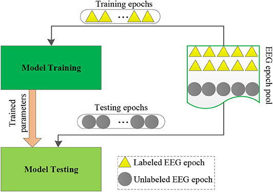
Figure 1. The classic diagnostic procedure for epilepsy.

Although existing intelligent models, for example, LMPROJ and A-TL-SSL-TSK, underlying the transfer learning framework are effective for epilepsy EEG signal recognition, there still exist some issues that should be further addressed.

• To tolerate the distribution difference between the source domain and the target domain, it is not enough to only minimize the marginal distribution difference between the two domains.

• Most of the existing models use only one source domain for knowledge transfer. That is to say, all available labeled data in the source domain are leveraged for model training. However, some labeled data may cause negative transfer.

Therefore, in this study, by overall considering the above two issues, we propose a new intelligent TSK fuzzy classifier (online selective transfer TSK fuzzy classifier with joint distribution adaption and manifold regularization, OS-JDA-MR-T-TSK-FC) for epilepsy EEG signal recognition. First, it further explores the marginal probability distribution adaption between the source domain and the target domain from two aspects. One is that it additionally introduces conditional probability distribution adaption to further minimize the distribution difference. The second is that it preserves manifold consistency underlying the marginal probability distribution. Second, it can selectively leverage knowledge from multiple source domains.

The following sections are organized as follows: in Data and Methods, we give the EEG data and our proposed method. In Results, we report the experimental results. Discussions about experimental results are presented in Discussions, and the whole conclusions are summarized in the last section.

Data and Methods

Data

In this study, we download very commonly used epilepsy EEG¹ data to verify our proposed intelligence model. The data from the University of Bonn is open to the public for scientific research. Table 1 gives the data archive and collection conditions. Additionally, Figure 2 illustrates the amplitudes during the collection procedure of one volunteer in each group. The original EEG data cannot be directly used for model training (Jiang et al., 2017b; Tian et al., 2019). We should employ feature extraction methods to extract robust features before model training.

TABLE 1

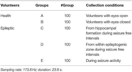
Table 1. Epilepsy EEG data archive and collection condition.

FIGURE 2

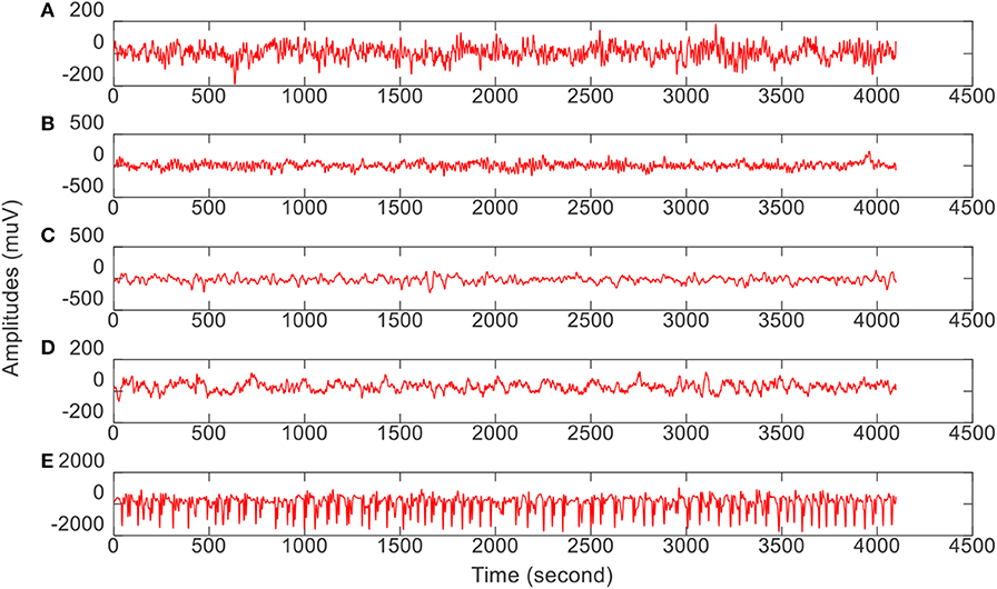
Figure 2. The amplitude of one volunteer in each group during the collection procedure. From top to bottom corresponds to (A–E), respectively.

Feature Extraction

Three feature extraction algorithms, that is, wavelet packet decomposition (WPD) (Li, 2011), short-time Fourier transform (STFT) (Pei et al., 1999), and kernel principal component analysis (KPCA) (Li et al., 2005), are employed to extract three kinds of features from the original epilepsy EEG signals.

• Wavelet Packet Decomposition

Wavelet packet decomposition is used to extract time-frequency features from epilepsy EEG signals. More specifically, the epilepsy EEG signals are disassembled into six different frequency bands with the Daubechies 4 wavelet coefficients. Each band is considered as one feature. Figure 3 illustrates the six features of group A.

• Short-Time Fourier Transform

FIGURE 3

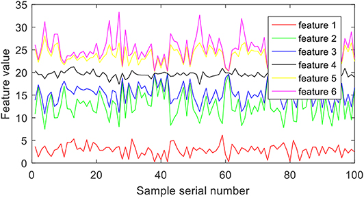
Figure 3. Features extracted by wavelet packet decomposition.

Short-time Fourier transform is used to extract frequency-domain features from epilepsy EEG signals. More specifically, the epilepsy EEG signals are disassembled into different local stationary signal segments, and then the Fourier transform is used to extract a group of spectra of the local segments, which are with evident time-varying characteristics at different times. Finally, six frequency bands are extracted from each group of spectra. Figure 4 illustrates the six features of group A.

• Kernel Principal Component Analysis

FIGURE 4

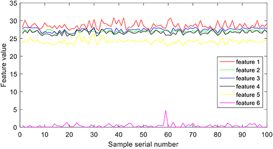
Figure 4. Features extracted by short time Fourier transform.

Kernel principal component analysis is used to extract time-domain features from epilepsy EEG signals. More specifically, the Gaussian function is chosen as the kernel to map the original features nonlinearly. Then six kinds of features are selected from the top six PC eigenvectors. Figure 5 illustrates the six features of group A.

FIGURE 5

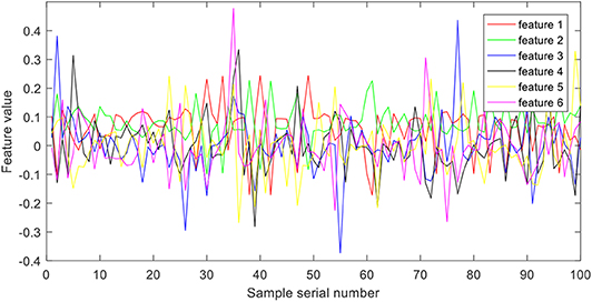
Figure 5. Features extracted by kernel principal component analysis.

Online Transfer Scenario Construction

We construct six online transfer scenarios from the EEG data after feature extraction (Table 2). Each scenario consists of five source domains as multiple source domains and one target domain. Specifically, two healthy groups (A, B) and three epileptic groups (C, D, E) are combined to generate six different pairs of combinations, that is, AC, AD, AE, BC, BD, and BE. Five pairs are alternatively selected from the six combinations as source domains, and the rest one is taken as the target domain such that each pair has the opportunity to become the target domain.

TABLE 2

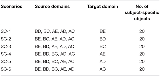
Table 2. Six online transfer scenarios.

In general, calibration in BCIs can be divided into two types, that is, offline calibration and online calibration (Jiang et al., 2020). Offline calibration means that we have obtained a pool of unlabeled EEG epochs. Some of unlabeled EEG epochs were labeled by experts to train a classifier. The unseen epochs then were classified by the trained classifier. Online calibration means that the training EEG epochs were obtained on-the-fly. That is to say, the classifier was trained online. Both calibration methods have their own advantages and disadvantages. For example, in offline calibration, unlabeled EEG epochs can be used to assist labeled ones to achieve classifier training, for example, semisupervised learning (Mallapragada et al., 2009; Zhang et al., 2013; Dornaika and El Traboulsi, 2016). Additionally, if necessary, we can easily obtain the label of any EEG epochs at any time. In online calibration, we not only have no unlabeled EEG epochs to be used for classifier training but also have little control on which epochs to see next. However, online calibration is more attractive because it is more in line with the needs of practical application scenarios. Therefore, in this study, we only consider online calibration for seizure classification. To simulate online calibration in the aforementioned six transfer scenarios, we first generate M = 20 subject-specific objects from the target domain. The online calibration flowchart is shown in Figure 6. We repeat all rounds 10 times to obtain statistically meaningful results, where each time has a random starting position m₀.

FIGURE 6

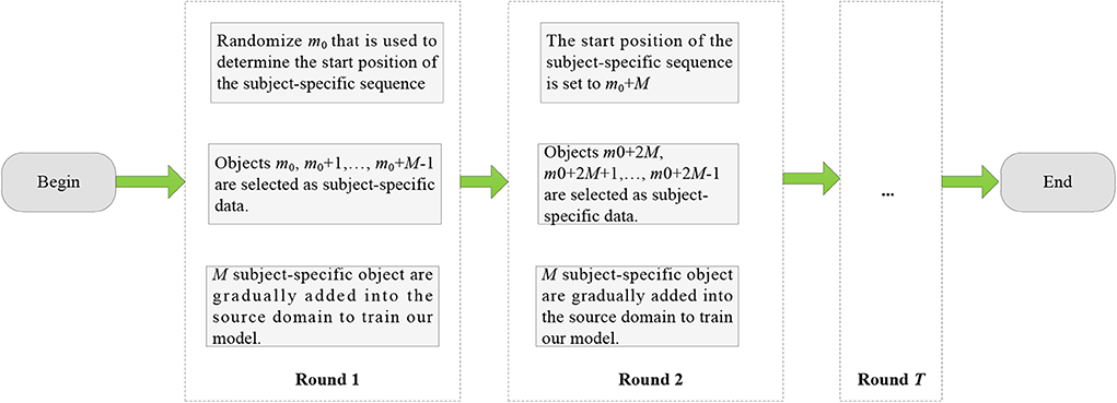
Figure 6. Online calibration flowchart.

Methods

In this section, we will elaborate the method we proposed for seizure classification. We first mathematically state the transfer problem, and then we give the online transfer learning framework and hence the online transfer TSK fuzzy classifier (OS-JDA-MR-T-TSK-FC). Lastly, we give the detailed algorithm steps of OS-JDA-MR-T-TSK-FC including how to select source domains.

Problem Statement

A domain Ψ = {X, P(x)} in the transfer learning or domain adaption scenario consists of a d-dimensional feature space ∈ R^d and a marginal distribution P(x), and a task Γ = {Y, P(y|x)} in the similar scenario consists of a one-dimensional label space Y and a conditional distribution P(y|x), where y ∈ Y. Suppose that Ψ_s and Ψ_t are two domains derived from Ψ, they are deemed to be different when X_s ≠ X_t and/or P_s(x) ≠ P_t(x). Homoplastically, two tasks Γ_s and Γ_t derived from Γ are different when Y_s ≠ Y_t and/or P_s(y|x) ≠ P_t(y|x).

Based on the above definitions, the target of OS-JDA-MR-T-TSK-FC is to train a predictive function on a source domain Ψ_s having N-labeled EEG epochs ${\left\{({\text{x}}_{\text{i}},y_i)\right\}}_{i=1}^N$ and a target domain Ψ_t having M-labeled EEG subject-specific epochs ${\left\{({\text{x}}_{\text{i}},y_i)\right\}}_{i=1}^M$ to predict the class label of a unseen epoch in the target domain with a low expected error under the hypotheses that Ψ_s = Ψ_t, Y_s = Y_t, P_s(x) ≠ P_t(x), and P_s(y|x) ≠ P_t(y|x).

OS-JDA-MR-T-TSK-FC

• Online Transfer Learning Framework

Because the classic one-order TSK fuzzy classifier (1-TSK-FC) (Deng et al., 2015; Jiang Y. et al., 2017a; Zhang J. et al., 2018; Zhang et al., 2019) is considered as the basic component of our online transfer learning framework, we first give some details about 1-TSK-FC before introducing our framework.

The kth fuzzy rule involved in 1-TSK-FC is formulated as the following if–then form:

$\begin{array}{l}\text{If }{x}_{i1}\text{is }{A}_1^k\wedge x_{i2}\text{is }{A}_2^k\wedge \dots \wedge x_{id}\text{is }{A}_d^k,\\ \text{then }{f}^k({\text{x}}_{\text{i}})=p_0^k+p_1^k{x}_{i1}+\dots +p_d^k{x}_{id},& (1)\end{array}$

where k = 1, 2, …, K, K represents the total number of fuzzy rules 1-TSK-FC uses. ${\text{x}}_{\text{i}}={\left[x_{i1},x_{i2},\dots ,x_{id}\right]}^T$ represents the ith object contains d features. $A_j^k$ in (1) represents a fuzzy set subscribed by x_ij for the kth fuzzy rule, and ∧ represents a fuzzy conjunction operator. Each fuzzy rule is premised on the feature space and maps the fuzzy sets in the feature space into a varying singleton represented by $f^k({\text{x}}_{\text{i}})$. After the steps of inference and defuzzification, the predictive function y^o(•) for an unseen object x is formulated as the following form:

$\begin{array}{ll}{y}^o(\text{x})={\displaystyle \sum _{k=1}^K}\left({\mu }^k(\text{x})/{\displaystyle \sum _{k^{\prime }=1}^K}{\mu }^{k^{\prime }}(\text{x})\right)f^k(\text{x})={\displaystyle \sum _{k=1}^K}(\tilde{\mu }(\text{x}))f^k(\text{x}),& (2)\end{array}$

in which the μ^k(x) is expressed as

$\begin{array}{ll}{\mu }^k(\text{x})={\prod }_{j=1}^d{\mu }_{A_j^k}(x_j),& (3)\end{array}$

where ${\mu }_{A_j^k}(x_j)$ can be expressed as the following form when the Gaussian kernel function is employed:

$\begin{array}{ll}{\mu }_{A_j^k}\left(x_j\right)=exp\left(-{\left(x_j-c_j^k\right)}^2/2{\left({\delta }_j^k\right)}^2\right),& (4)\end{array}$

where $c_j^k$ and ${\delta }_j^k$ are two parameters representing the kernel center and kernel width, respectively. Therefore, training of 1-TSK-FC means to find optimal $c_j^k$, ${\delta }_j^k$ in the if parts, and ${\text{p}}^k={\left[p_0^k,p_1^k,\dots ,p_d^k\right]}^T$ in the then parts. Referring to the literature (Zhang et al., 2019), we know that parameters in the if parts can be trained by clustering techniques. For instance, $c_j^k$ and ${\delta }_j^k$ can be trained by fuzzy c-means (FCM) (Gu et al., 2017) as

$\begin{array}{ll}{c}_j^k={\displaystyle \sum _{i=1}^N}{\mu }_{ik}{x}_{ij}/{\displaystyle \sum _{i=1}^N}{\mu }_{ik}& (5)\end{array}$

$\begin{array}{ll}{\delta }_j^k=h{\displaystyle \sum _{i=1}^N}{{\mu }_{ik}(x_{ij}-c_j^k)}^2{\displaystyle \sum _{i=1}^N}{\mu }_{ik},& (6)\end{array}$

where μ_ik is the fuzzy membership degree of x_i belonging to the kth cluster. h is a regularized parameter that can be always set to 0.5 according to the suggestions in Jiang Y. et al. (2017a). When $c_j^k$ and ${\delta }_j^k$ in the if parts are determined by FCM or other similar techniques, for an object x_i in the training set, let

$\begin{array}{ll}{\text{x}}_e={(1,{({\text{x}}_{\text{i}})}^T)}^T,& (\mathrm{7.a})\end{array}$

$\begin{array}{ll}{\tilde{\text{x}}}_i^k={\tilde{\mu }}^k({\text{x}}_i){\text{x}}_e,& (\mathrm{7.b})\end{array}$

$\begin{array}{ll}{\text{x}}_{gi}={({({\tilde{\text{x}}}_i^1)}^T,{({\tilde{\text{x}}}_i^2)}^T,\dots ,{({\tilde{\text{x}}}_i^K)}^T)}^T,& (\mathrm{7.c})\end{array}$

$\begin{array}{ll}{\text{p}}^k={(p_0^k,p_1^k,\dots ,p_d^k)}^T,& (\mathrm{7.d})\end{array}$

$\begin{array}{ll}{\text{p}}_g={({({\text{p}}^1)}^T,{({\text{p}}^2)}^T,\dots ,{({\text{p}}^K)}^T)}^T,& (7.e)\end{array}$

then we can rewrite the predictive function y^o(·) in (2) as the following form:

$\begin{array}{ll}{y}^o({\text{x}}_i)={\text{p}}_{\text{g}}^T{\text{x}}_{gi}& (8)\end{array}$

Referring to Zhou et al. (2017) and Zhang Y. et al. (2018), we formulate an objective function as follows to solve p_g:

$\begin{array}{ll}{J}_{1-order-TSK-Fc}({\text{p}}_g)=\frac{1}{2}{({\text{p}}_{g,c})}^T{\text{p}}_{g,c}+\frac{\eta }{2}{\displaystyle \sum _{i=1}^N}{\Vert {({\text{p}}_g)}^T{\text{x}}_{gi}-y_i\Vert }^2,& (9)\end{array}$

where the first $\frac{1}{2}{({\text{p}}_g)}^T{\text{p}}_g$ is a generalization term, the second is a square error term, and η > 0 is balance parameter used to control the tolerance of errors and the complexity of 1-TSK-FC. By setting the partial derivative of the objective function w.r.t p_g to zero, that is, ∂J_{1−order−TSK−FS}(p_g)/∂p_g = 0, we can compute p_g analytically as

$\begin{array}{ll}{\text{p}}_g={\left({\text{I}}_{k(d+1)\times k(d+1)}+{\displaystyle \sum _{i=1}^N}{\text{x}}_{gi}{({\text{x}}_{gi})}^T\right)}^{-1}\times \left(\eta {\displaystyle \sum _{i=1}^N}{\text{x}}_{gi}{y}_i\right).& (10)\end{array}$

In this study, 1-TSK-FC is taken as the basic learning component to support the transfer learning framework. Many previous works (Yang et al., 2014; Jiang et al., 2017c) explored the marginal distribution adaption between the source domain and the target domain for transfer learning. In our framework, we introduce conditional distribution adaption to further minimize the distribution difference. Additionally, we impose manifold consistency on the marginal distribution. Therefore, the transfer learning framework can be formulated as

$\begin{array}{l}f=arg{\displaystyle \underset{f}{min}}[{\displaystyle \sum _{i=1}^N}\ell (f({\text{x}}_i),y_i)+{\omega }_t{\displaystyle \sum _{i=N+1}^{N+M}}\ell (f({\text{x}}_i),y_i)]\\ +{\lambda }_1\left[D(J_s,J_t)\right]+{\lambda }_2\left[M(P_s,P_t)\right],& (11)\end{array}$

where ω_t in the first term is the overall weights of the specific-subject objects. Generally, ω_t should be larger than 1 so that more emphasis is given to objects in Ψ_s than Ψ_t. Therefore, we set ω_t to ω_t = max(2, σ · N/M). λ₁ and λ₂ are regularization parameters. The first term contains two parts: the first is to measure the loss on Ψ_s, and the second is to measure the loss in Ψ_t. The second one is the joint distribution adaption term, and the third one is the manifold regularization term. Below, we will explain how to embody them formally.

• Objective function of OS-JDA-MR-T-TSK-FC

Under the framework shown in (11), we specify each term to get the objective function of our online transfer TSK fuzzy classifier OS-JDA-MR-T-TSK-FC.

Loss Function

The squared loss is taken as the loss function to measure the sum of squared training errors on both Ψ_s and Ψ_t; hence, the first term in (11) can be formulated as

$\begin{array}{l}{\displaystyle \sum _{i=1}^N}{(f({\text{x}}_i)-y_i)}^2+{\omega }_t{\displaystyle \sum _{i=N+1}^{N+M}}{(f({\text{x}}_i)-y_i)}^2\\ ={\displaystyle \sum _{i=1}^N}{({\text{p}}_g^T{\text{x}}_{gi}-y_i)}^2+{\omega }_t{\displaystyle \sum _{i=N+1}^{N+M}}{({\text{p}}_g^T{\text{x}}_{gi}-y_i)}^2,& (12)\end{array}$

where $f(\text{x})={\text{p}}_g^T{\text{x}}_{gi}$ is the predictive function of 1-TSK-FC. Suppose we have a diagonal matrix Θ in which each element is defined as

$\begin{array}{ll}\Theta (i,i)=\{\begin{array}{ll}1& 1\le i\le N\\ {\omega }_t& N+1\le i\le N+M\end{array}.& (13)\end{array}$

By submitting (13) to (12), then (12) can be rewritten as

$\begin{array}{l}{\displaystyle \sum _{i=1}^N}{({\text{p}}_g^T{\text{x}}_{gi}-y_i)}^2+{\omega }_t{\displaystyle \sum _{i=N+1}^{N+M}}{({\text{p}}_g^T{\text{x}}_{gi}-y_i)}^2\\ ={\displaystyle \sum _{i=1}^{N+M}}\Theta (i,i){({\text{p}}_g^T{\text{x}}_{gi}-y_i)}^2\\ =({\text{y}}^T-{\text{p}}_g^T{\text{X}}_g^T)\Theta (\text{y}-{\text{X}}_g{\text{p}}_g),& (14)\end{array}$

where ${\text{X}}_g={\left[{\text{X}}_{g1},\dots ,{\text{X}}_{gN},\dots ,{\text{X}}_{g(N+M)}\right]}^T$ in which each element ${\text{X}}_{gi}$ is derived from ${\text{X}}_i$ by using (7.c).

Joint distribution adaptation

As all we know that even EEG epoch features in Ψ_s and Ψ_t are extracted in the same way, the joint distributions (marginal and conditional distributions) between Ψ_s and Ψ_t are generally different. In order to meet practical requirements, we assume that P_s(x) ≠ P_t(x) and P_s(y|x) ≠ P_t(y|x). Therefore, a joint distribution adaptation should be designed to minimize the distribution similarity (distance) D(J_s, J_t) between Ψ_s and Ψ_t.

First, the projected MMD (Gangeh et al., 2016; Jia et al., 2018; Lin et al., 2018) is employed to the marginal distribution similarity D(P_s, P_t) between Ψ_s and Ψ_t. As a result, D(P_s, P_t) can be expressed as

$\begin{array}{ll}D(P_t,P_s)={\left[\frac{1}{N}{\displaystyle \sum _{i=1}^N}f({\text{x}}_i)-\frac{1}{M}{\displaystyle \sum _{i=N+1}^{N+M}}f({\text{x}}_i)\right]}^2={\text{p}}_g^T{\text{X}}_g\Phi {\text{X}}_g{\text{p}}_g,& (15)\end{array}$

where Φ is the MMD matrix, which can be defined as

$\begin{array}{ll}\Phi (i,j)=\{\begin{array}{ll}1/N^2,& 1\le i\le N,\text{1}\le j\le N\\ 1/M^2,& N+\text{1}\le i,j\le N+M\\ -1/NM& \text{otherwise}.\end{array}& (16)\end{array}$

Second, we suppose that Ψ_s,c belongs to Ψ_s and its objects are selected by {x_i|x_i ∈ Ψ_s ∧ y_i = c}, and Ψ_t,c belongs to Ψ_t and its objects are selected by {x_i|x_i ∈ Ψ_t ∧ y_i = c}, where c means the cth class in one domain. Also, for the source domain, N_c is used to denote the number of objects in the cth class, and for the specific-subject objects in the target domain, M_c is used to denote the number of objects in the cth class. Hence, D(Q_s, Q_t) can be expressed as

$\begin{array}{l}D(Q_t,Q_s)={\displaystyle \sum _{c=1}^2}{[\frac{1}{N_c}{\displaystyle \sum _{{\text{x}}_i\in {\Omega }_{s,c}}}f({\text{x}}_i)-\frac{1}{M_c}{\displaystyle \sum _{{\text{x}}_j\in {\Omega }_{t,c}}}f({\text{x}}_j)]}^2\\ ={\displaystyle \sum _{c=1}^2}{[\frac{1}{N_c}{\displaystyle \sum _{{\text{x}}_i\in {\Omega }_{s,c}}}{\text{p}}_g^T{\text{x}}_{gi}-\frac{1}{M_c}{\displaystyle \sum _{{\text{x}}_j\in {\Omega }_{t,c}}}{\text{p}}_g^T{\text{x}}_{gj}]}^2,\\ ={\displaystyle \sum _{c=1}^2}{\text{p}}_g^T{\text{X}}_g{\Delta }_c{\text{X}}_g{\text{p}}_g,\\ ={\text{p}}_g^T{\text{X}}_g\Delta {\text{X}}_g{\text{p}}_g,& (17)\end{array}$

where $\Delta ={\displaystyle \sum _{c=1}^2}{\Delta }_c$ and Δ_c is an MMD matrix defined as follows:

$\begin{array}{ll}{\Delta }_c(i,j)=\{\begin{array}{ll}1/N_c^2& {\text{x}}_i,{\text{x}}_j\in {\Omega }_{s,c}\\ 1/M_c^2& {\text{x}}_i,{\text{x}}_j\in {\Omega }_{t,c}\\ -1/N_c{M}_c& {\text{x}}_i\in {\Omega }_{s,c},{\text{x}}_j\in {\Omega }_{t,c}\\ & \text{or }{\text{x}}_i\in {\Omega }_{t,c},{\text{x}}_j\in {\Omega }_{s,c}\\ 0& \text{otherwise}\end{array}& (18)\end{array}$

According to the probability theory, the joint adaption D(J_s, J_t) = D(P_s, P_t)+D(Q_s, Q_t) so that the joint distribution adaptation can be formulated as

$\begin{array}{l}D(J_s,J_t)=D(P_t,P_s)+D(Q_t,Q_s)\\ ={\text{p}}_g^T{\text{X}}_g\Phi {\text{X}}_g{\text{p}}_g+{\text{p}}_g^T{\text{X}}_g\Delta {\text{X}}_g{\text{p}}_g,\\ ={\text{p}}_g^T{\text{X}}_g(\Phi +\Delta ){\text{X}}_g{\text{p}}_g.& (19)\end{array}$

Manifold regularization

In the manifold assumption (Lin and Zha, 2008; Chen and Wang, 2011; Geng et al., 2012), it is assumed that if two objects x_i and x_j are very close in the intrinsic geometry in terms of P(x_i) and P(x_j), then the corresponding Q(y_i|x_i) and Q(y_j|x_j) are considered as being similar. That is to say, for the objects in Ψ_s and the calibration objects in Ψ_t, if they are in a manifold, it is expected that their output (conditional probability distribution) differences should be as small as possible. Therefore, the manifold regularization can be formulated as follows under geodesic smoothness,

$\begin{array}{l}M(P_s,P_t)={\displaystyle \sum _{i=1}^{N+M}}{\displaystyle \sum _{j=1}^{N+M}}{(f({\text{x}}_i)-f({\text{x}}_j))}^2{w}_{ij}\\ ={\displaystyle \sum _{i=1}^{N+M}}{\displaystyle \sum _{j=1}^{N+M}}f({\text{x}}_i)l_{ij}f({\text{x}}_j)\\ ={\displaystyle \sum _{i=1}^{N+M}}{\displaystyle \sum _{j=1}^{N+M}}{\text{p}}_g^T{\text{x}}_{gi}{l}_{ij}{\text{p}}_g^T{\text{x}}_{gj}\\ ={\text{p}}_g^T{\text{X}}_g\text{L}{\text{X}}_g{\text{p}}_g,& (20)\end{array}$

Where, W = [w_ij]_(N+M)×(N+M) is the graph affinity matrix in which each element is defined as

$\begin{array}{ll}{w}_{ij}=\{\begin{array}{ll}cos({\text{x}}_i,{\text{x}}_j)& \text{if }{\text{x}}_i\in {\xi }_{\nu }({\text{x}}_j)\text{ or }{\text{x}}_j\in {\xi }_{\nu }({\text{x}}_i)\\ 0& \text{otherwise}\end{array},& (21)\end{array}$

Where, ξ_ν(x_i) represents a set of v-nearest neighbors of object x_i. L = [l_ij]_(N+M)×(N+M) is the corresponding normalized graph Laplacian matrix of W, which can be computed by L = I − D^−1/2WD^−1/2, where D is the degree matrix in which each diagonal element d_ii is computed by $\sum _{j=1}^{N+M}{w}_{ij}$.

By embedding the manifold regularization into the transfer learning framework, the marginal probability distributions of objects in the target domain and the source domain are fully utilized to guarantee the consistency between the predictive structure of the decision function f and the intrinsic manifold data structure.

By substituting (14), (19), and (20) into our transfer learning framework shown in (12), we can obtain a transfer learning model, that is, OS-JDA-MR-T-TSK-FC as

$\begin{array}{l}f=arg{\displaystyle \underset{f}{min}}[({\text{y}}^T-{\text{p}}_g^T{\text{X}}_g^T)\Theta (\text{y}-{\text{X}}_g{\text{p}}_g)\\ +{\text{p}}_g^T{\text{X}}_g{\lambda }_1(\Phi +\Delta ){\text{X}}_g{\text{p}}_g+{\text{p}}_g^T{\text{X}}_g{\lambda }_2\text{L}{\text{X}}_g{\text{p}}_g],\\ =arg{\displaystyle \underset{f}{min}}[({\text{y}}^T-{\text{p}}_g^T{\text{X}}_g^T)\Theta (\text{y}-{\text{X}}_g{\text{p}}_g)\\ +{\text{p}}_g^T{\text{X}}_g({\lambda }_1(\Phi +\Delta )+{\lambda }_2\text{L}){\text{X}}_g{\text{p}}_g].& (22)\end{array}$

We can deduce a closed-form solution of p_g for the objective function in (26) by setting its derivative w.r.t p_g to zero as

$\begin{array}{ll}{\text{p}}_g={\left[{\text{X}}_g^T(\Theta +{\lambda }_1\Phi +{\lambda }_1\Delta +{\lambda }_2\text{L}){\text{X}}_g\right]}^{-1}{\text{X}}_g^T\Theta \text{y}.& (23)\end{array}$

Algorithm of OS-JDA-MR-T-TSK-FC

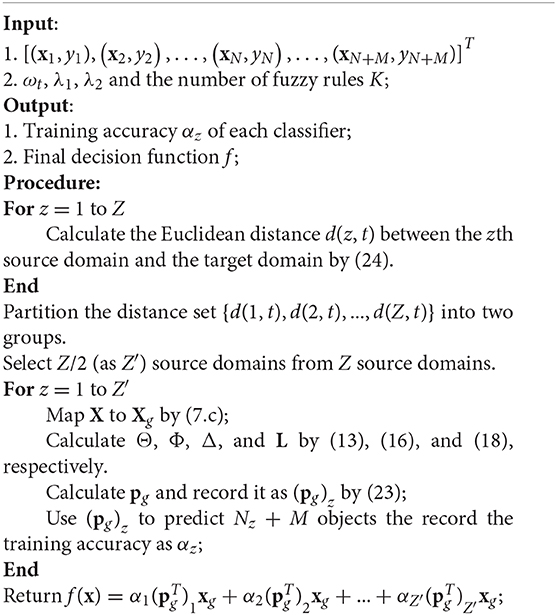
Different from most of the existing transfer models, OS-JDA-MR-T-TSK-FC can leverage knowledge from multiple source domains. However, as we know, too many source domains will improve computational complexity. Additionally, some source domains having significant differences with the target domain may bring some negative transfer knowledge. Therefore, according to Wu et al. (2017), we adopt a distance-based schema to select relative source domains.

We use v_z,c to denote the mean vector of each class in the zth source domain, where z = 1,2,…, Z. Similarly, v_t,c is used to denote the mean vector of each class in the target domain. The Euclidean distance between the zth source domain and the target domain can be computed as

$\begin{array}{ll}d(z,t)={{\displaystyle \sum _c}\Vert {\text{v}}_{z,c}-{\text{v}}_{t,c}\Vert }^2.& (24)\end{array}$

With (24), we can get a distance set {d(1, t), d(2, t), …, d(Z, t)} that contains Z domain distances. The distance set then is partitioned by k-means to k groups (in this study, k is set to 2), and the source domains are selected from the cluster who has the smallest center.

As a whole, the training of OS-JDA-MR-T-TSK-FC contains three parts: the first one is source domain selection, the second one is model training on a source domain combining with the target domain, and the last is classifier combination. Algorithm 1 shows the detailed training steps of OS-JDA-MR-T-TSK-FC.

ALGORITHM 1

Algorithm 1: OS-JDA-MR-T-TSK-FC

OS-JDA-MR-T-TSK-FC can also be used for multiclassification tasks. According to Zhou et al. (2017), we can convert y from the space R to the space R^C by that y_ij = 1 if y(x_i) = j, and y_ij = 0 otherwise, where i = 1, 2, …, N + M, j = 1, 2, …, C, and C represents the number of classes. Thus, the label space becomes $\text{Y}={\left[{\text{y}}_1,\dots ,{\text{y}}_N,\dots ,{\text{y}}_{N+M}\right]}^T\in R^C$, and ${\text{p}}_g$ is also converted from R^d+1 to R^(d+1)×C.

Results

Experiment setups and comparison results will be reported in this section.

Setups

For fair, we introduce three baselines and one transfer learning algorithm for comparison study. The three baselines all use 1-TSK-FC for training. But their training sets are different.

(1) Baseline 1 (BL1). Its training set consists of the five source domains directly connected, and its testing set is the target domain. Therefore, BL1 is considered as a calibration-independent classifier, which does not use the subject-specific data in the target domain for training.

(2) Baseline 2 (BL2). It uses only subject-specific calibration EEG data in the target domain for training. Its testing set is the unlabeled data in the target domain. Therefore, BL2 is considered as a source domain-independent classifier, which does not consider the EEG data in the source domains at all.

(3) Baseline 3 (BL3). BL3 is trained on five training sets, receptively. Each set consisted of a source domain and the subject-specific data in the target domain. The five trained models are finally combined by a weight schema that is also used in Algorithm 1. Its testing set is the unlabeled data in the target domain

(4) Transfer support vector machine (TSVM) (Chapelle et al., 2008). It trains five TSVM classifiers by combining unlabeled EEG data in the target domain for semisupervised learning. The five trained models are finally combined by a weight schema that is also used in Algorithm 1.

(5) ARRLS (Long et al., 2014). It trains five ARRLS classifiers by combining unlabeled EEG data in the target domain for supervised learning. The five trained models are finally combined by a weight schema that is also used in Algorithm 1.

Experimental Results

In this section, we report the experimental results from several aspects, that is, classification performance, interpretability, and robustness.

• Classification Performance

Table 3 shows the average classification performance of the six scenarios in the KPCA feature space, PWD feature space, and STFT feature space, respectively. Table 4 shows the classification performance on KPCA features. Table 5 shows the classification performance on PWD features, and Table 6 shows the classification performance on STFT features. The best results are marked in bold.

• Interpretability

TABLE 3

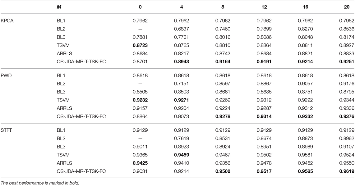
Table 3. Average classification performance of the six scenarios in three feature spaces.

TABLE 4

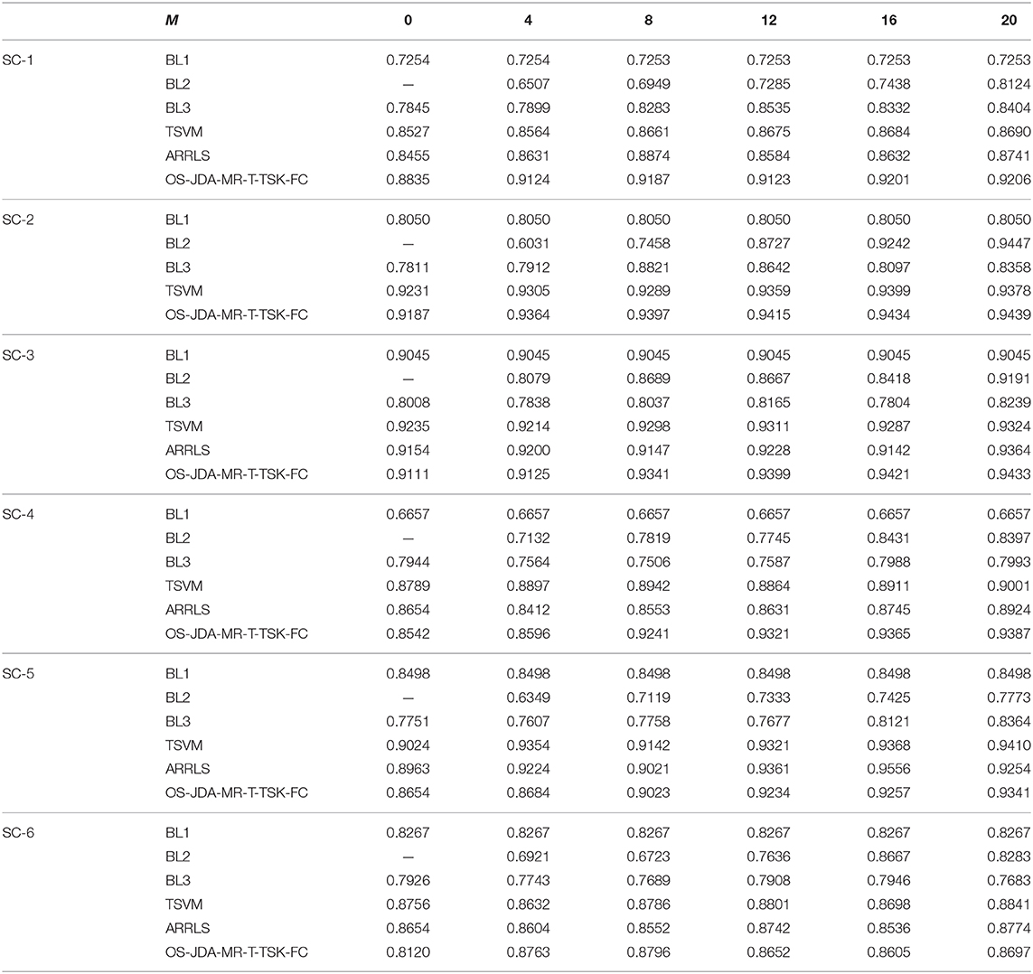
Table 4. Classification performance on six scenarios in the KPCA feature space.

TABLE 5

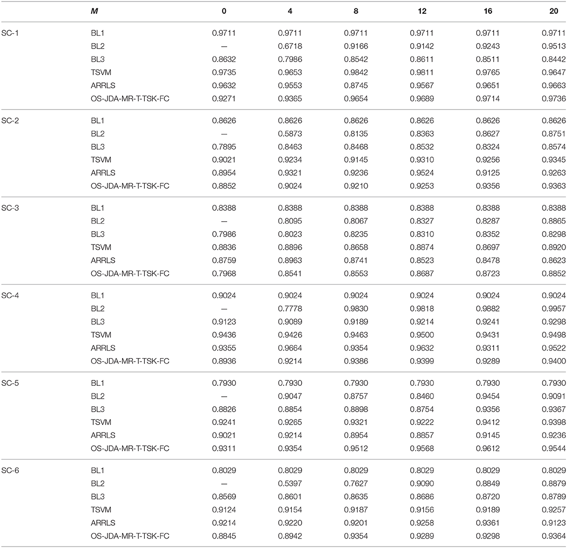
Table 5. Classification performance on six scenarios in the WPD feature space.

TABLE 6

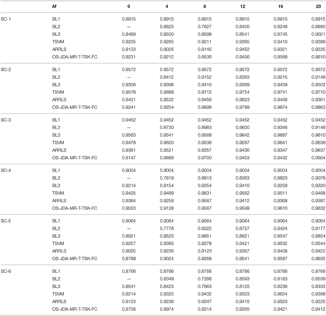
Table 6. Classification performance on six scenarios in the STFT feature space.

Unlike TSVM that works in a black-box manner, the proposed OS-JDA-MR-T-TSK-FC has high interpretability because 1-TSK-FC is taken as the basic component. Table 7 shows the five trained fuzzy rules (antecedent and consequent parameters) on SC-1 in the KPCA feature space.

• Robustness

TABLE 7

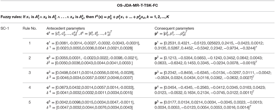
Table 7. Fuzzy rules trained on SC-1 in the KPCA feature space.

From the objective function of OS-JDA-MR-T-TSK-FC, we see that there are three parameters, that is, ω_t (σ), λ₁, and λ₂ that should be fixed before a classification task. So, we should consider the robustness OS-JDA-MR-T-TSK-FC to them. The sensitivity analysis results are shown in Figure 7.

FIGURE 7

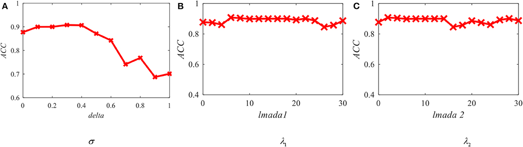
Figure 7. Average accuracy of OS-JDA-MR-T-TSK-FC in the KPCA feature space with different parameters. (A) Robustness w.r.t delta; (B) robustness w.r.t lmada 1; (C) robustness w.r.t lmada 2.

Discussions

We observe from Table 3 that the proposed OS-JDA-MR-T-TSK-FC wins the best average performance across the six transfer scenarios in all feature spaces when the number of specific-subject objects is more than 4. Especially compared with the three baselines, the advantages are more obvious.

Moreover, the classification results in Tables 4–6 also exhibit the following four characteristics:

• BL1 does not use the specific-subject objects, so its accuracy is independent on M, whereas the other four classifiers depend on M, and it is intuitive that they gradually perform better than BL1 with the increasing of M.

• BL2 is only trained by the subject-specific objects. Therefore, BL2 becomes unusable when M is set to 0. But BL1, BL3, TSVM, and OS-JDA-MR-T-TSK-FC can work because, except subject-specific objects, they also leverage training objects from the source domains. Compared with other algorithms, when M is too small, BL2 performs so badly because it cannot get enough training patterns from subject-specific objects.

• When M is set to 0, TSVM always achieves the best performance. With the subject-specific objects gradually added into the training set, OS-JDA-MR-T-TSK-FC soon performs better than TSVM, which indicates that significant differences exist among the domains. Hence, a domain-dependent classifier, for example, TSVM is not very expected in our online transfer scenarios.

• When one batch (four subject-specific objects are taken as a batch in our experiments) or at most two batches of subject-specific objects are added into the training set, the classification performance of OS-JDA-MR-T-TSK-FC becomes stable. That is to say, the number of subject-specific objects OS-JDA-MR-T-TSK-FC needs is very small. So, OS-JDA-MR-T-TSK-FC meets the practical requirements because subject-specific objects are very few in real-world applications.

In addition to classification performance, interpretability is also a main characteristic of the proposed OS-JDA-MR-T-TSK-FC. From Table 7, we see that it generates five interpretable fuzzy rules on SC-1 in the KPCA feature space. Each feature in a fuzzy rule can be interpreted as the energy of an EEG signal band, and each fuzzy membership function is endowed with a linguistic description. For example, “x₁ is $A_1^k$” in the antecedent of a fuzzy rule can be interpreted as “the energy of an EEG band is a litter high,” where the term “a little high” can be replaced by others such as “a litter low,” “medium,” or “high.” In this way, suppose I am an expert from the field of EEG signal analysis, I assign five kinds of linguistic descriptions to each fuzzy membership function, that is, “low,” “a little low,” “medium,” “a little high,” and “high.” Therefore, for the first fuzzy rule in Table 7, it can be interpreted as follows:

If the energy of an EEG signal band (band 1) is “high,” and the energy of an EEG signal band (band 2) is “a little low,” and the energy of an EEG signal band (band 3) is “low,” and the energy of an EEG signal band (band 4) is “low,” and the energy of an EEG signal band (band 5) is “low,” and the energy of an EEG signal band (band 6) is “low,” then the consequent of the first fuzzy rule can be expressed as:

$f^1(\text{x})=0.2531+0.4321x_1-0.5123x_2+0.2562x_3+0.2415x_4-0.0423x_5+0.0012x_6+0.3153$−0.5278x₁+0.4452x₂−0.5342x₃+0.2342x₄−0.9734x₅−0.3244x₆.

From Figure 6, we observe that O-T-TSK-FC is robust to σ in the range of [0.1, 0.4], to λ₁ in the range of (Geng et al., 2012; Jiang et al., 2017c), and to λ₂ in the range of (Ghosh-Dastidar et al., 2008; Mallapragada et al., 2009), respectively.

Conclusions

In this study, we propose a seizure classification model OS-JDA-MR-T-TSK-FC using an online selective transfer TSK fuzzy classifier with a joint distribution adaption and manifold regularization. We use epilepsy EEG signals provided by the University of Bonn as the original data and construct six transfer scenarios in three kinds of feature spaces to demonstrate the promising performance of OS-JDA-MR-T-TSK-FC. We also generate four baselines and introduce a transfer SVM model for fair comparison. The experimental results show that OS-JDA-MR-T-TSK-FC performs better than baselines and the introduced two transfer models. However, in this study, we only consider how to select the source domains. Recent studies show that dynamically selecting useful samples from the source domain can effectively induce the learning on the target domain. Therefore, in our future work, we will try to develop a mechanism, for example, classification error consensus to select most useful samples from the source domain.

Data Availability Statement

The original EEG data are available in http://www.meb.unibonn.de/epileptologie/science/physik/eegdata.html.

Author Contributions

YZ designed the whole algorithm and experiments. ZZ, HB, and WL contributed on code implementation, and LW gave some suggestions to the writing.

Funding

This work was supported in part by the National Natural Science Foundation of China under Grants No. 81873915, 817017938, by Ministry of Science and Technology Key Research and Development Program of China under Grants no. 2018YFC0116902.

Conflict of Interest

The authors declare that the research was conducted in the absence of any commercial or financial relationships that could be construed as a potential conflict of interest.

Acknowledgments

We thank the reviewers whose comments and suggestions helped improve this manuscript.

Footnote

1. ^http://www.meb.unibonn.de/epileptologie/science/physik/eegdata.html.

References

Chapelle, O., Sindhwani, V., and Keerthi, S. S. (2008) Optimization techniques for semi-supervised support vector machines. J. Mach. Learn. Res. 9, 203–233.

Google Scholar

Chen, K., and Wang, S. (2011). Semi-supervised learning via regularized boosting working on multiple semi-supervised assumptions. IEEE Trans. Pattern Anal. Mach. Intell. 33, 129–143. doi: 10.1109/TPAMI.2010.92

PubMed Abstract | CrossRef Full Text | Google Scholar

Deng, Z., Cao, L., Jiang, Y., and Wang, S. (2015). Minimax probability TSK fuzzy system classifier: a more transparent and highly interpretable classification model. IEEE Trans. Fuzzy Systems 23, 813–826. doi: 10.1109/TFUZZ.2014.2328014

CrossRef Full Text | Google Scholar

Dornaika, F., and El Traboulsi, Y. (2016). Learning flexible graph-based semi-supervised embedding. IEEE Trans. Cybern. 46, 206–218. doi: 10.1109/TCYB.2015.2399456

PubMed Abstract | CrossRef Full Text | Google Scholar

Gangeh, M. J., Tadayyon, H., Sannachi, L., Sadeghi-Naini, A., Tran, W. T., and Czarnota, G. J. (2016). Computer aided theragnosis using quantitative ultrasound spectroscopy and maximum mean discrepancy in locally advanced breast cancer. IEEE Trans. Med. Imaging 35, 778–790. doi: 10.1109/TMI.2015.2495246

PubMed Abstract | CrossRef Full Text | Google Scholar

Geng, B., Tao, D., Xu, C., Yang, L., and Hua, X. (2012). Ensemble manifold regularization. IEEE Trans. Pattern Anal. Mach. Intell. 34, 1227–1233. doi: 10.1109/TPAMI.2012.57

PubMed Abstract | CrossRef Full Text | Google Scholar

Ghosh-Dastidar, S., Adeli, H., and Dadmehr, N. (2008). Principal component analysis-enhanced cosine radial basis function neural network for robust epilepsy and seizure detection. IEEE Trans. Biomed. Eng. 55, 512–518. doi: 10.1109/TBME.2007.905490

PubMed Abstract | CrossRef Full Text | Google Scholar

Gu, X., Chung, F., Ishibuchi, H., and Wang, S. (2017). Imbalanced TSK fuzzy classifier by cross-class bayesian fuzzy clustering and imbalance learning. IEEE Trans. Systems Man Cybern. Systems 47, 2005–2020. doi: 10.1109/TSMC.2016.2598270

CrossRef Full Text | Google Scholar

Jia, X., Zhao, M., Di, Y., Yang, Q., and Lee, J. (2018). Assessment of data suitability for machine prognosis using maximum mean discrepancy. IEEE Trans. Ind. Electron. 65, 5872–5881. doi: 10.1109/TIE.2017.2777383

CrossRef Full Text | Google Scholar

Jiang, Y., Deng, Z., Chung, F., and Wang, S. (2017a). Realizing two-view TSK fuzzy classification system by using collaborative learning. IEEE Trans. Systems Man Cybern. Systems 47, 145–160. doi: 10.1109/TSMC.2016.2577558

CrossRef Full Text | Google Scholar

Jiang, Y., Deng, Z., Chung, F. L., Wang, G., Qian, P., Choi, K. S., et al. (2017b). Recognition of Epileptic EEG Signals Using a Novel Multiview TSK Fuzzy System. IEEE Trans. Fuzzy Systems 25, 3–20. doi: 10.1109/TFUZZ.2016.2637405

CrossRef Full Text | Google Scholar

Jiang, Y., Wu, D., Deng, Z., Qian, P., Wang, J., Wang, G., et al. (2017c). Seizure classification from EEG signals using transfer learning, semi-supervised learning and TSK fuzzy system. IEEE Trans. Neural Sys. Rehabil. Eng. 25, 2270–2284. doi: 10.1109/TNSRE.2017.2748388

PubMed Abstract | CrossRef Full Text | Google Scholar

Jiang, Y., Zhang, Y., Lin, C., Wu, D., and Lin, C. (2020). EEG-based driver drowsiness estimation using an online multi-view and transfer TSK fuzzy system. IEEE Trans. Intell. Transportation Systems. 1–13. doi: 10.1109/TITS.2020.2973673

CrossRef Full Text | Google Scholar

Jiang, Z., Chung, F., and Wang, S. (2019). Recognition of multiclass epileptic EEG signals based on knowledge and label space inductive transfer. IEEE Trans. Neural Sys. Rehabil. Eng. 27, 630–642. doi: 10.1109/TNSRE.2019.2904708

PubMed Abstract | CrossRef Full Text | Google Scholar

Li, J., Tao, D., Hu, W., and Li, X. (2005). “Kernel principle component analysis in pixels clustering,“ in The 2005 IEEE/WIC/ACM International Conference on Web Intelligence (WI'05), (Compiegne: IEEE). 786–789.

Google Scholar

Li, S. (2011). ”Speech Denoising Based on Improved Discrete Wavelet Packet Decomposition,“ in 2011 International Conference on Network Computing and Information Security (Guilin: IEEE), 415–419. doi: 10.1109/NCIS.2011.182

CrossRef Full Text | Google Scholar

Lin, T., and Zha, H. (2008). Riemannian manifold learning. IEEE Trans. Pattern Anal. Mach. Intell. 30, 796–809. doi: 10.1109/TPAMI.2007.70735

PubMed Abstract | CrossRef Full Text | Google Scholar

Lin, W., Mak, M., and Chien, J. (2018). Multisource I-vectors domain adaptation using maximum mean discrepancy based autoencoders. IEEE/ACM Trans. Audio Speech Lang. Proc. 26, 2412–2422. doi: 10.1109/TASLP.2018.2866707

CrossRef Full Text | Google Scholar

Long, M., Wang, J., Ding, G., Pan, S. J., and Yu, P. S (2014). Adaptation regularization: a general framework for transfer learning. IEEE Trans. Knowl. Data Eng. 26, 1076–1089. doi: 10.1109/TKDE.2013.111

CrossRef Full Text | Google Scholar

Mallapragada, P. K., Jin, R., Jain, A. K., and Liu, Y. (2009). SemiBoost: boosting for semi-supervised learning. IEEE Trans. Pattern Anal. Mach. Intell. 31, 2000–2014. doi: 10.1109/TPAMI.2008.235

PubMed Abstract | CrossRef Full Text | Google Scholar

Parvez, M. Z., and Paul, M. (2016). Epileptic seizure prediction by exploiting spatiotemporal relationship of EEG signals using phase correlation. IEEE Trans. Neural Systems Rehabil. Eng. 24, 158–168. doi: 10.1109/TNSRE.2015.2458982

PubMed Abstract | CrossRef Full Text | Google Scholar

Pei, S. C., Yeh, M. H., and Luo, T. L. (1999). Fractional Fourier series expansion for finite signals and dual extension to discrete-time fractional Fourier transform. IEEE Trans. Signal Proc. 47, 2883–2888. doi: 10.1109/78.790671

CrossRef Full Text | Google Scholar

Tian, X., Deng, Z., Ying, W., Choi, K. S., Wu, D., Qin, B., et al. (2019). Deep multi-view feature learning for EEG-based epileptic seizure detection. IEEE Trans. Neural Systems Rehabil. Eng. 27, 1962–1972. doi: 10.1109/T.N.S.R.E.2019.2940485

PubMed Abstract | CrossRef Full Text | Google Scholar

Van Hese, P., Martens, J., Waterschoot, L., Boon, P., and Lemahieu, I. (2009). Automatic detection of spike and wave discharges in the EEG of genetic absence epilepsy rats from strasbourg. IEEE Trans. Biomed. Eng. 56, 706–717. doi: 10.1109/TBME.2008.2008858

PubMed Abstract | CrossRef Full Text | Google Scholar

Wang, Y., Chen, Y., Su, A. W., Shaw, F., and Liang, S. (2016). Epileptic pattern recognition and discovery of the local field potential in amygdala kindling process. IEEE Trans. Neural Systems Rehabil. Eng. 24, 374–385. doi: 10.1109/TNSRE.2015.2512258

PubMed Abstract | CrossRef Full Text | Google Scholar

Wu, D., Lawhern, V. J., Gordon, S., Lance, B. J., and Lin, C. (2017). Driver drowsiness estimation from EEG signals using online weighted adaptation regularization for regression (OwARR). IEEE Trans. Fuzzy Systems 25, 1522–1535. doi: 10.1109/TFUZZ.2016.2633379

CrossRef Full Text | Google Scholar

Yang, C., Deng, Z., Choi, K. S., Jiang, Y., and Wang, S. (2014). Transductive domain adaptive learning for epileptic electroencephalogram recognition. Artif. Intell. Med. 62, 165–177. doi: 10.1016/j.artmed.2014.10.002

PubMed Abstract | CrossRef Full Text | Google Scholar

Zhang, J., Deng, Z., Choi, K., and Wang, S. (2018). Data-driven elastic fuzzy logic system modeling: constructing a concise system with human-like inference mechanism. IEEE Trans. Fuzzy Sys. 26, 2160–2173. doi: 10.1109/TFUZZ.2017.2767025

CrossRef Full Text | Google Scholar

Zhang, Y., Dong, J., Zhu, J., and Wu, C. (2019). Common and special knowledge-driven TSK fuzzy system and its modeling and application for epileptic EEG signals recognition. IEEE Access 7, 127600–127614. doi: 10.1109/ACCESS.2019.2937657

CrossRef Full Text | Google Scholar

Zhang, Y., Ishibuchi, H., and Wang, S. (2018). Deep takagi–sugeno–kang fuzzy classifier with Shared Linguistic Fuzzy Rules. IEEE Trans. Fuzzy Systems 26, 1535–1549. doi: 10.1109/TFUZZ.2017.2729507

CrossRef Full Text | Google Scholar

Zhang, Z., Chow, T. W. S., and Zhao, M. (2013). Trace ratio optimization-based semi-supervised nonlinear dimensionality reduction for marginal manifold visualization. IEEE Trans. Knowl. Data Eng. 25, 1148–1161. doi: 10.1109/TKDE.2012.47

CrossRef Full Text | Google Scholar

Zhou, T., Chung, F., and Wang, S. (2017). Deep TSK fuzzy classifier with stacked generalization and triplely concise interpretability guarantee for large data. IEEE Trans. Fuzzy Sys. 25, 1207–1221. doi: 10.1109/TFUZZ.2016.2604003

CrossRef Full Text | Google Scholar