Making online polls more accurate: statistical methods explained

Arletti, Alberto; Tanturri, Maria Letizia; Paccagnella, Omar

doi:10.3389/fpos.2025.1592589

REVIEW article

Front. Polit. Sci., 11 July 2025

Sec. Political Science Methodologies

Volume 7 - 2025 | https://doi.org/10.3389/fpos.2025.1592589

This article is part of the Research TopicMethods in political science – Innovation & DevelopmentsView all 8 articles

Making online polls more accurate: statistical methods explained

Alberto Arletti^*

Maria Letizia Tanturri

Omar Paccagnella

Department of Statistical Sciences, University of Padova, Padova, Italy

Online data has the potential to transform how researchers and companies produce election forecasts. Social media surveys, online panels, and even comments scraped from the internet can offer valuable insights into political preferences. However, such data is often affected by significant selection bias, as online respondents may not be representative of the overall population. At the same time, traditional data collection methods are becoming increasingly cost-prohibitive. In this scenario, scientists need instruments to be able to draw the most accurate estimate possible from samples drawn online. This paper provides an introduction to key statistical methods for mitigating bias and improving inference in such cases, with a focus on electoral polling. Specifically, it presents the main statistical techniques, categorized into weighting, modeling, and other approaches. It also offers practical recommendations for drawing estimates with measures of uncertainty. Designed for both researchers and industry practitioners, this introduction takes a hands-on approach, with code available for implementing the main methods.

1 Introduction

Random sampling, one of the most powerful tools in scientific research, was first introduced in 1934. The idea is simple. Given a small portion of individuals in a group, it is possible to obtain a reliable estimate for the parameter of interest for the whole population, such as the population mean. A random sample, or probability sample—adjectives which will be used interchangeably in the text—possesses therefore the seemingly magical power of achieving an estimate even with few values of n, the sample size, compared to N, the population size (Smith, 1976). The key to such a feat of random sampling lies in managing to obtain a sample which is entirely random with respect to all aspects that might influence the parameter of interest. To do so, researchers often need to know the probability of each individual in the population to join the survey, a value called inclusion probability. If such value is known and is not zero, the sample can be considered a representative probability sample.

Although straightforward, respecting such a requirement in practice can be a major issue. This is especially true when drawing measurements of complex human phenomena, such as voting behavior. As stated by Kruskal and Mosteller (1979) “the idea will rarely work in a complicated social problem because we always have additional variables that may have important consequences for the outcome” (p. 249).

The delicate complexity of social problems requires random sampling to follow extra steps in order to obtain effective randomness in the sample, and therefore maintain its status as the “dominating” sampling mechanism. For example, when contacting citizens in order to measure their voting intentions for an upcoming election, randomness could be achieved by calling phone numbers at random, given a list of all phone addresses in a given area (method referred to as Random Digit Dialling, or RDD). But what about people who can't answer the phone, for a variety of reasons that could be connected with their choice of vote, and therefore generate bias in the final outcome? In other words, “polling of humans is far from the simple random sampling described in many statistics textbooks” (Gelman, 2021, p. 69).

The issue of achieving randomization when human factors are at play is further hampered by another important aspect: declining response rates. The decrease has been abundantly reported (Brick, 2011), with a recent example being the decline from 60% in 2004 to 40% in 2024 in the European Social Survey (European Social Survey, 2024). This decline applies to electoral polls as well (Gelman, 2021). As people are seemingly uninterested in answering field researchers, two consequences appear: Firstly, a non-response bias is introduced in electoral polls (Shirani-Mehr et al., 2018), which is to say that the individuals who do not respond could be systematically different from those who do respond. Secondly, conducting research becomes more expensive, as more and more people need to be contacted to obtain a representative sample (Baker et al., 2013b). Representative surveys can also be more expensive, even without considering response rates. For example, Unangst et al. (2020) reports the cost for a single interview to be 10$ when conveniently obtained from the internet, with little guarantees of randomness, while the cost climbs to 192$ for the more selection-safe face-to-face approach. In addition to the prohibitive costs, given the complexity of social sciences and the increasing rates of non-response, one might legitimately question whether a truly random sample is still achievable at all. These two considerations led some researchers to state that there is no such thing as a “random sample” anymore (Bailey, 2023; Beaumont and Haziza, 2022) or, humorously, that “non-random samples are almost everywhere” (Meng, 2018, p. 718). These two consequences have led researchers and polling companies to increasingly turn to alternative methods of sampling. In the following, we introduce non-probability sampling as a pragmatic response to the challenges and limitations of probability-based approaches.

1.1 Non-probability samples

Given the aforementioned problems, researchers might need alternative methods for data collection. To the rescue come non-probability samples, or non-random samples. Non-probability samples are all samples that come from a vast number of techniques used to obtain data, from snowball sampling (Dusek et al., 2015) to asking people's opinion on social media (Alexander et al., 2020) to scraping web pages (Schirripa Spagnolo et al., 2025), to many others. Such samples are cheaper and more convenient to obtain, and therefore a very popular choice for researchers and practitioners.

In the social sciences, non-probability samples can be advantageous due to their versatility, low cost, and possibility of being employed where other methods often cannot. In particular, speed can be a remarkable quality. For example, the influx of online non-probability data can allow feats such as using Facebook Advertising Platform to nowcast the distribution of migrant groups in the United States, as in Alexander et al. (2020) and Zagheni et al. (2017). In another example, the stream of non-representative Twitter data has been used to provide fast-updated estimates of pre-electoral polls for the US elections (Beauchamp, 2017). Non-probability samples can also be used to make updated forecasts when more recent census data is unavailable, such as in using Google searches to forecast birth rates (Billari et al., 2016). Continuing, non-random sampling can often be the only viable strategy to examine hard-to-reach populations, as for example using mobile and landline in De Vries et al. (2021), using LinkedIn as in Dusek et al. (2015), or using the social media platforms Vkontakte e Odnoklassniki (Rocheva et al., 2022). Migrants are an especially salient case of such populations, which might not fit in the traditional administrative or random sampling schemes. For example, Zagheni et al. (2014) used localized tweets to draw a non-random sample used to infer migration patterns, while Jacobsen and Kühne (2021) used a tracking app for the same aim. Finally, it is clear that using social media, a case of non-probability sampling, offers the advantage of smaller prices and a relatively large pool of individuals to draw from. While most samples obtained online can often be considered non-probabilistic in nature, it is worth noting that some online probability samples exist, as Blom et al. (2016).

1.1.1 Pollings and the shortcoming of non-probability samples

Even though it is clear that non-probability samples such as opt-in online panels or social media data can be a game changer in many scenarios, the significant drawbacks of selection bias, which might result in less accurate results, must be accounted for Callegaro et al. (2014b). Selection bias can be defined as systematic differences between the sampled and target populations, due to the fact that the survey was accessible to a section of the population only, for example, internet users only or Facebook users only. Non-probability samples are non-representative as they carry selection bias, which leads to a violation of the canon of randomness in some measure.

Because non-probability samples contain this selection, drawn estimates, such as the predicted share of votes for a said party, are not reliable, as in they do not represent the target population of interest, but rather the selected subgroup from data was extracted (e.g., Facebook users who happened to be online at the time of the survey). Therefore, while selection is used in a random sample to select a sample which is random in all its characteristics with respect to the interest statistics, non-random samples are vulnerable to the adverse effect of selection (Kruskal and Mosteller, 1979, p. 246). Some examples of such violations of the pure assumptions of probability sampling are nonresponse, incomplete coverage of the population, and measurement errors (Brick, 2011). The effect is that the “magical” quality of random samples is not applicable anymore, and suddenly the small size n of the sample is unable to measure correctly the large N of the interest population (Meng, 2022). Therefore, this has led the American Association for Public Opinion Research (AAPOR) in 2010 (Baker et al., 2010) and again in 2013 (Baker et al., 2013a, p. 12) to state that “researchers should avoid non-probability opt-in-panels when a key research objective is to accurately estimate population values... claims of representativeness should be avoided when using these sample sources.”

Another issue is that respondents in non-probability surveys, such as those collected via social media or online panels, tend to provide less informative responses compared to more involved methods like face-to-face interviews. For instance, Fricker et al. (2005) and Heen et al. (2014) document “depressed responses” in such settings, evidenced by answer clustering around the middle of the scale, reduced differentiation, and fewer extreme opinions.

Arguably, the field where non-probability samples' shortfalls have generated the strongest shockwave is electoral polling (Evans and Mathur, 2018; Zagheni and Weber, 2015; Shirani-Mehr et al., 2018). As put eloquently in a 2018 review: “Polls have had a number of high-profile misses in recent elections. Political polls have staggered from embarrassment to embarrassment in recent years” (Prosser and Mellon, 2018, p. 757). Famous examples are the 2016 presidential race (Kennedy et al., 2018) [which has been named “a black eye” for polling (Gelman, 2021, p. 67)], the 2016 Brexit referendum (Financial Times, 2016), and the 2023 Turkish general elections (Selcuki, 2023). Generally, the failure of those polls is mainly attributed to the use of non-probability samples (Gelman, 2021), as such samples have been reported as less accurate compared to probability sources (Sohlberg et al., 2017; Sturgis et al., 2018). Nonetheless, the trend does not seem to be stopping for the rise of non-probability samples in electoral polling as well (Callegaro et al., 2014a). A failure in an electoral prediction bears a higher cost for the public image of the discipline. After all, “election polling is arguably the most visible manifestation of statistics in everyday life” (Shirani-Mehr et al., 2018, p. 608). Election polling is almost the most salient because poll-based forecasts are compared to actual election outcomes (Gelman, 2021).

Researchers might end up stuck between a rock and a hard place. Random samples can hardly be completely trustworthy and require heavy costs compared to the cheaper non-probability alternatives (Tam and Clarke, 2015). On the other hand, non-probability samples carry important challenges for inference. Given these premises, what should researchers do with the abundant quantities of non-random samples available, such as Twitter posts, Google searches, online, and opt-in panels, etc.? It is clear that the need for reliable approaches to draw valuable inferences from non-probability samples is pressing and might bring great benefits to the academic community. After all, “Great advances of the most successful sciences—astronomy, physics, chemistry were and are achieved without probability sampling.” (Kish, 1965, pp. 28–29).

From this scenario, the need for statistical methods used to draw valid inferences from non-probability social science data emerges as paramount for the whole scientific community. Statistical methods could aim at reducing or acting as a counterweight to the distortion or bias present in such non-probability samples. In other words, the estimated value would be closer to the true population value after applying the estimation method, in the form of calibration or correction.

Given the potential of non-probability data sources, such as social media online surveys, for the social sciences and opinion research, such as electoral polling, it is crucial to explore statistical methods that reduce bias and improve accuracy in such datasets. This work aims to assist researchers and practitioners by outlining key statistical techniques for correcting non-probability data, focusing on reducing distortion or bias. It provides an accessible overview of these methods, their assumptions, and practical implementation, serving as a reliable guide for selecting and applying the appropriate approach in their analyses.

2 Data availability scenarios in non-probability sampling

Addressing selection bias in non-probability samples requires appropriate statistical methods, but their applicability depends on the available population information. Researchers may find themselves in different data availability scenarios when working with non-probability samples, which are briefly illustrated here.

In the simplest case, only sample data is available, with no population reference (e.g., hard-to-reach groups like migrants, where census data is lacking). More commonly, researchers also have population totals, as in electoral data, which may be available in marginal (e.g., total voters by sex or region) or cross-tabulated form (e.g., female voters by region). Lastly, some non-probability samples can be paired with a (often smaller-sized) probability sample (Tutz, 2023; Rafei et al., 2022). The present contribution focuses on the second case, where marginal or cross-tabulated totals are available. The first case allows little room for correction, while the third involves distinct challenges and is less common in electoral poll practice.

In the second setting, population information is available as either marginal totals or cross-tabulated census data. This can be represented as a dataset with a target variable Y, a set of covariates X with p parameters, and a p-sized vector T(X) containing population totals for each variable in X. When complete cross-tabulated census data is available, the researcher has two datasets: (1) A non-representative sample containing Y and predictors (also named covariates in the text) X (n rows). (2) A representative dataset of the full population (N rows) with covariates X, but without Y. These datasets can be concatenated with an indicator variable S, where S = 1 for sampled units and S = 0 otherwise (see Figure 1).

Figure 1

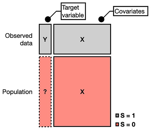
Figure 1. Schematic representation of the variables in the considered dataset.

An additional important concept is population cells. Any population, such as voters in a country, can be divided into non-overlapping cells. Each cell represents a unique category in the population, defined by a specific combination of categorical X variables. For example, a cell might be male, 30–45 years old, voter. The total number of cells is given by the product of the levels of available categorical variables. For instance, if gender (2 levels) and employment status (3 levels) are available, the population is divided into 2 × 3 = 6 cells. The X covariates can also be political affiliation variables in the case of electoral polling, such as party affiliation or the party voted in the previous elections.

Finally, hands-on practice enhances the learning of new methods. To complement the theoretical discussion, this introduction is accompanied by a sample dataset and code implementations for most methods presented. This allows readers to grasp both the technical details and practical application. The code and data are available on GitHub: nonign_sel_companion.

3 Weighting

Weighting, or calibration weighting, first introduced by Deville and Särndal (1992), is considered one of the most important methods for correcting a non-representative sample (Valliant, 2020). In weighting, the individual observations are up or down weighted so their distribution is adapted to be more similar to the distribution of a representative sample or of the census. In their most basic idea, if the sample has way more males than females compared to the known national totals, then male observations can be down-weighted. This class of methods can also be referred to as “pseudo-weighting” or “quasi-randomization” (Valliant, 2020). This is due to the fact that in random sampling, observations in the sample are weighted by the inverse of their inclusion probability, which is known (see Horvitz and Thompson, 1952). In the case of non-random sampling, the inclusion probabilities are not known and are to be estimated. Therefore, weighting is used in trying to approximate sampling weights in a manner that resembles what is done in probability sampling. In the case of unknown inclusion probabilities, or non-random samples, weighting can be obtained with one, or a combination of raking, propensity scoring, and matching.

3.1 Raking (iterative proportional fitting)

Iterative Proportional Fitting, or Raking, Deming and Stephan (1940) is a weighting method which is used to weight a dataframe so that the X variables' marginals match the corresponding population marginals. This is done in the case of multiple marginal distributions, for example, gender and region. The term iterative is used to refer to the process that is used to obtain the weighting, which can be described in simple words as adjusting the weights iteratively, making them more similar to the marginals at each iteration until convergence (Stephan, 1942).

The goal of raking is to assign weights w₁ … w_j … w_n to each row in the sample so that the weighted sums match known population totals from the census. For the covariate p, this can be expressed as:

\begin{array}{l} \sum_{j = 1}^{n} w_{j} x_{j, p} = T (X_{p}) . & (1) \end{array}

Here, T(X_p) is the population total for the p-th covariate, and x_{j, p} represents the value of the p-th covariate for row j. The estimated population mean ( $\hat{μ} (Y)$ ) is then obtained as:

\begin{array}{l} \hat{μ} (Y) = \frac{1}{n} \sum_{j = 1}^{n} y_{j} w_{j} . & (2) \end{array}

This formula allows the estimation of the population total for the target variable, such as the share of votes. If one would like to obtain measures of uncertainty around such an estimate, a common practice is to use a bootstrap or similar resampling approaches (Kolenikov, 2010). Alternatively, a direct expression to obtain raking variance is provided in Deville and Särndal (1992).

Raking is a very simple weighting method that only requires the marginal distributions to be employed, and is especially useful in the case where only marginal totals are available (see Section 2), or in cases where the number of observations in each cell is small. Nonetheless, it can suffer from a series of limitations. To begin with, the raking to the marginals does not take into account possible higher-level interactions between the raking variables. This can be an issue, making the weighing less accurate compared to the real population distribution. A proposed solution to this problem is multilevel calibration weighting, an approach by Ben-Michael et al. (2021). While raking matches the marginal distributions of the raked variables only, it might not be able to balance higher-order interactions. Multilevel calibration weighting aims at solving that, behaving similarly to raking but adding some approximate balance for interaction, prioritizing lower-order interactions. In addition, if the raking variables do not fully account for the inclusion probability, the method becomes inconsistent. Finally, it should be noted that the weights produced by raking can have very high (or very low) values, making the practice unreliable. One possible solution is “trimming” the weights, or constraining the weights to be in a certain range of values. Such a solution is also implemented directly in the R command for raking anesrake (Pasek, 2018).

3.2 Propensity score adjustment

Propensity Score Adjustment is a class of adjustment methods that relies on the estimation of the probability of inclusion in the non-probability sample. The main method, discussed here, is often referred as Propensity Score-based Inverse Probability Weighting (PS-IPW) (Zou et al., 2016).

PS-IPW works through the use of a second representative sample, with common covariates to the non-probability sample, where the target Y variable is missing (Schonlau and Couper, 2017; McPhee et al., 2022). Such a sample can be generated knowing the census cross-tabulated totals, if those are available. To do so, it would be sufficient to generate a dataframe where each column corresponds to a census cross-tabulated variable, and the number of rows that belong in each cell corresponds to, or is proportional to, the known population total. The two datasets are temporarily binned into a single frame, as described in Section 2 and Figure 1. Then, the method builds a weighted logistic regression model to estimate the probability of an observation being in a non-probability sample. Here, the regression weights correspond to the known inclusion probabilities in the reference sample, while non-sampled observations receive a weight of 1. Inclusion probabilities in the reference sample correspond to the known probability of individual j of being included in the sample, which generally accompany a representative sample. If the reference sample has been generated from the cross-tabulated census values, then the inclusion probability of a row j belonging to cell c is just the inverse of the numerosity of that cell. The regression can be described as:

\begin{array}{l} logit (P (S = 1 | X)) = β_{0} + β^{T} X . & (3) \end{array}

The predicted values of the weighted regression, which can be set as ${\hat{π}}_{j} = logit (P (S_{j} = 1 | x_{j}))$ , are then inverted and used to estimate the population mean.

\begin{array}{l} {\hat{μ}}_{PS-IPW} (Y) = \frac{1}{n} \sum_{j = 1}^{n} \frac{1}{{\hat{π}}_{j}} y_{j} . & (4) \end{array}

This last formula is the same as the famous Horvitz-Thompson estimator (Horvitz and Thompson, 1952), with the difference that the weights are not known from the sample design, but are estimated from the data. It is also similar to Equation 2, with the difference that the $\frac{1}{{\hat{π}}_{j}}$ values are estimated differently from w_j. Such a probability estimated from the data is called the propensity score. What this achieves is an estimation of the inclusion probabilities, which are unknown, from the observed data. The propensity score represents the conditional probability of being included in the survey given an individual's covariate profile.

For a measure of uncertainty of this estimate, variance estimates can be obtained through a Taylor linearization approximation (Valliant et al., 2013, p. 426) or through a Jackknife approximation (Valliant, 2020, p. 8).

One topic of discussion regards which model to choose in order to obtain propensity scores. While logistic regression is a very popular method, some authors argue that it is insufficient in cases such as where the propensity score shows a non-linear function. In this regard, Lee et al. (2010) compares the performance of different methods to obtain propensity scores. They compare both logistic regression with Classification and Regression Trees (CART) models, and find that logistic regression's performance can deteriorate in case of non-additivity and non-linearity. Therefore, choosing a flexible or non-parametric approach to model propensity scores can be advantageous. For example, Rafei et al. (2020) uses Bayesian Additive Regression Trees (BART) to model inclusion probabilities (see also Elliott et al., 2010 for Bayesian modeling of this kind). Furthermore, attention should be dedicated to choosing the appropriate variables to correctly model inclusion probabilities. To this task, variable selection methods such as in Ferri-García and Rueda (2022) can be employed.

Once an appropriate model has been selected to capture the selection mechanism and there are no empty cells in the data, the PS-IPW can be used to build reliable estimators. A first assumption of this approach is that every unit in the population has a non-zero propensity score. A second important assumption is that the covariates X should include all relevant confounders (Lee and Valliant, 2009). The main danger in using this method emerges when the selected X variables do not fully account for the sample selection mechanism, or in other words, there is significant selection bias that cannot be controlled by the available covariates. In that case, adjusting for the propensity score will not produce unbiased estimates of the treatment effect. A further requirement of PS-IPW is called “common support” and requires that the distribution of the covariates in the reference sample is similar to the distribution in the sample to be adjusted. For example, there should not be population cells completely absent from the non-probability sample (Valliant, 2020). Pseudo-inclusion probabilities are typically estimated using weighted logistic regression (Lee and Valliant, 2009).

4 Modeling

Another popular approach to adjust non-probability surveys and reduce selection bias is modeling. In this case, the non-random sample is employed to train a model used to predict the dependent variable for each cell of the missing rows, corresponding to the population. This approach is also called superpopulation model estimation (Valliant, 2020), model-based predictive inference (Buelens et al., 2018), or model-based estimation (Wu, 2022). In modeling, the y_i values of the non-sampled units are predicted with a variety of methods trained on the sampled units. In this way, the value for the total population is considered the union of both the sampled and non-sampled units. That is, the non-sampled units correspond to all individuals who are in the target population, but not in the sample.

4.1 Post-stratification

Superpopulation methods are therefore comprised of two steps, a first modeling step, where the model is estimated from the observed data, and a post-stratification step, where the value is predicted for each cell of the population. The sum of all predicted values for all cells gives the estimated value for the entire population. After modeling, the post-stratification step allows for balancing for sample discrepancy.

An estimate of the population mean for a given cell of the population, y_c, where the subscript c indicates the cell, can be obtained by first estimating a model between Y and X in the sample, for example, a linear regression. This can be described as:

\begin{array}{l} logit (P (Y = 1 | X)) = β_{0} + β^{T} X . & (5) \end{array}

Then, the cell total can be obtained using the following formula:

\begin{array}{l} \hat{μ} (Y_{c}) = \frac{N_{c}}{N} (β_{0} + β^{T} X_{c}) & (6) \end{array}

where N_c is the known size of the population cell c, X_c indicates the matrix of covariates data for the cell c, and $\hat{β}$ are the estimated regression coefficients. The estimate for the whole population will be the sum of all cell totals, so that $\hat{μ} (Y) = \sum_{c} \hat{μ} (Y_{c})$ .

While the post-stratification adjustment step remains the same across applications, what can be changed is the model used for prediction. A simple linear model can be substituted with more complicated or non-linear models. In this regard, Ferri-García et al. (2021) and Castro-Martín et al. (2020) examine the use of machine-learning models as prediction models, such as neural networks and decision trees. However, when predictors are demographic categorical variables, a hierarchical model is most effective, and such adjustment is referred to as Multilevel Regression and Post-stratification (MRP). MRP is not of recent development, with Gelman (1997) being the original proposer of the method. Nonetheless, MPR is one superpopulation method that is frequently used with non-representative surveys (McPhee et al., 2022; Si, 2020). In MRP, a multilevel regression model is used to estimate the outcome variable using a larger number of auxiliary variables and their interactions than is possible with standard weighting methods. The particularity of MRP is that it performs a cell-based (sub-group) estimation, and the hierarchical component (with Bayesian prior in its original specification, see Li and Si, 2022) regularizes the model and allows for borrowing of information.

MRP is a key method in the field, and it provides several advantages over post-stratification with a simple linear regression. To best understand the mechanics of MPR, it can be useful to examine the following formula for estimating the population mean using MPR (Si, 2020, p. 5):

\begin{array}{l} {\hat{μ}}_{MRP} (Y) = \sum_{c} \frac{N_{c}}{N} \frac{\hat{μ} (Y_{c}) + δ_{c} \hat{μ} (Y)}{1 + δ_{c}}, where δ_{c} = \frac{σ_{c}^{2}}{n_{c} σ_{Y}^{2}} . & (7) \end{array}

Here, as in Equation 6 the subscript c indicates a post-stratification cell, $\hat{μ} (Y_{c})$ is the model estimate for cell c, N_c is the size of cell c in the population, $\hat{μ} (Y)$ is the estimated population mean, $σ_{c}^{2}$ is the variance of the outcome variable for cell c, n_c is the sample size for cell c and $σ_{Y}^{2}$ is the outcome between-cell variance. Between-cell variance is a measure of how much the mean of Y differs from one cell to another, reflecting systematic differences between groups defined by the stratifying variables (e.g., age, gender, region). Therefore, what this formula tells us is that the less information we have on cell c, both in terms of sample size and variety, the more we are going to “borrow” from the other cells. This method is especially effective in non-probability online panel samples or social media samples, where it's quite often the case to have cells with very few observations.

For uncertainty measures on the population estimates of both post-stratification and MRP usually a Bayesian approach with posterior draws is usually preferred (Lopez-Martin et al., 2022).

For illustration purposes, an example of an electoral poll adjustment using Bayesian MRP is presented in Figure 2. In the plot, the blue dotted and dashed line represents the unadjusted sample mean, while the red dotted line represents the true population value for the share of votes of the center-left coalition in the 2022 Italian elections. The black dashed line represents instead the adjusted population estimate using MRP. In each subplot, the marginal probability of each subpopulation cell to vote for that party is plotted, together with credibility interval bands.

Figure 2

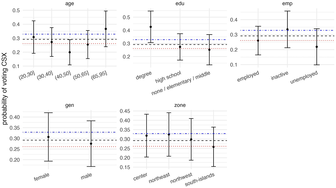
Figure 2. Application example of MRP.

It has been noted that post-stratification is useful in reducing selection bias and correcting imbalances in the sample composition. One advantage of such estimators is their ability to reduce bias (Kim et al., 2021). In this regard, the method has shown to be capable of impressive bias-correcting performances in election forecasting, for example in Wang et al. (2015). Nonetheless, when drawing inference with such method, some factors come into play to determine its performance. The first factor is the need for high-quality predictive post-stratification variables, or, in other words, variables with a strong relationship with the outcome variable. Authors have reported how poorly predictive auxiliary information might have an important effect on the final outcome (Si, 2020), and that variables chosen for post-stratification are more relevant than the model used for estimation (Prosser and Mellon, 2018). For example, Buttice and Highton (2013) examines the correlates of MRP performance in various scenarios. The authors examine how MRP accuracy of estimates of election results varies as the strength of the relationship between voting opinion and state-level covariates increases. They observe that as the strength of the relationship between opinion and the state-level covariates increases, then also MRP estimates get closer to the true values. This is not seen with the same strength for the individual-level covariates.

The requirement for high-quality post-stratification variables can be challenging when the census is limited. The requirement to have cross-tabulated population tables can be daunting, especially as the number of covariates increases. Therefore, it is often the case that variables useful for adjustment are not included in the census, such as party identification or previous vote (Gelman, 2021). Usually, due to non-availability in census, post-survey adjustments are limited to basic demographics such as age, gender, race, and education from large-scale government surveys (Chen et al., 2019). Moreover, for the case of electoral polling, these problems can be exacerbated for practitioners working outside of the United States. For example, pollsters in the United States can access party registration information, which is generally unavailable in other countries (Prosser and Mellon, 2018). Therefore, MRP has generally been applied so far in election forecasts for a few countries (Leemann and Wasserfallen, 2017). As a possible solution, Kastellec et al. (2015) suggests expanding the post-stratification table by incorporating a survey that includes one or more non-census variables, which can aid in adjusting for discrepancies between the sample and the target population. Such practice can be referred to as “embedded MRP” or e-MRP (Li and Si, 2024; Ornstein, 2023).

5 Other methods

5.1 Statistical matching

Statistical Matching, also known as Sample Matching or Mass Imputation, is a technique that can be applied both before the sample is selected (Cornesse et al., 2020; Bethlehem, 2016) or after the non-probability sample is already obtained (Mercer et al., 2018). The approach for the second case, the one of interest for the purpose of the present work, is attributed to Rivers (2007). Similarly to Propensity Score Adjustment, it requires a probability sample where the target variable does not need to be measured, but where there are matching covariates. The reference sample is treated as a target, where each row of the target is paired with the closest observation in the non-probability sample. The “matching” observation is chosen to be an observation that has the strongest similarity in the covariates. A Euclidean distance metric can be used (Cornesse et al., 2020), as well as any sort of similarity matrix, such as one obtained from a Random Forest (Mercer et al., 2018). Alternatively, a nearest neighbor approach can be useful, especially in the cases of continuous variables or categorical variables with many ordinal levels (Chen and Shao, 2000). The closest match is chosen for each row of the reference sample, and any remaining observation that has not been paired is discarded. Sequentially, each observation in the target dataframe is matched one at a time, and the most similar case is chosen among the cases which has not been matched previously. Then, the statistics of interest are obtained using the target variable y of the matched cases. In other words, each row of the target reference sample is substituted with the most similar observation in the non-probability case.

The main limitation of matching is that, in order to obtain a meaningful matching, a sufficiently large set of variables should be available in the required probability sampling. Most often, these variables should be different than the common demographic variables and might not be present in the available census. Otherwise, other forms of adjustment would be more straightforward. For the case of electoral polling, obtaining a reference sample with such characteristics can be challenging.

5.2 Inverse sampling

Inverse Sampling is presented for the estimation of non-probability big data samples in Kim and Wang (2019). The idea of inverse sampling is to leverage the large n of the non-probability sample to make a sub-selection. The first-phase sample consists of big data, named A, which is affected by selection bias. The second-phase sample, named A₂, is a subset of the first-phase sample, designed to adjust for this selection bias. To extract the subsample, inclusion probabilities proportional to the importance weights are used for selection. External information from a reference sample or from the census is used to correct for selection bias in the second step.

5.3 Doubly-robust estimation

Doubly-Robust estimation or Doubly-Robust Post-stratification (DRP) is substantially a combination between weighting, seen in Section 3, and modeling, seen in Section 4. The fundamental idea is to combine the two components, a propensity score component and modeling with a post-stratification component. When estimating a propensity score model, the specified model might be incorrect; for example, it might ignore interactions that influence the selection mechanism. The same might be for the modeling approach, where the chosen model might not be the best fit to describe the relationship between the target variable (Y) and the available covariates (X) (Tan, 2007). In DRP, the final estimate will be correct as the sample size increases even if one of the two models, either the modeling or the propensity score model, is incorrect or misspecified (Theorem 2; Chen et al., 2020). This guarantees further protection against bias. Similarly to DR-IPW, imagine a second reference sample where Y is missing. We call the non-probability sample A and the reference probability sample B. To obtain DRP, two models are fitted,

1. A propensity score model on the probability of j-th being included in A, using, for example, a weighted logistic regression as in Equation 4. The predicted propensity score is again ${\hat{π}}_{j}$ for row j.

2. A model of the relationship between the target Y and the covariates X, using A data only, as in Equation 5. The predicted value of y for row j by this model is indicated as ŷ_j.

For the case of a linear model, the final DRP population estimate is obtained by:

\begin{array}{l} \begin{array}{l} {\hat{μ}}_{DR} (Y) = \frac{1}{\sum_{i \in A} 1 / {\hat{π}}_{i}} \sum_{i \in A} \frac{1}{{\hat{π}}_{i}} (y_{i} - {\hat{y}}_{j}) + \frac{1}{N} \sum_{c} N_{c} (β_{0} + β^{T} X_{c}) . \end{array} & (8) \end{array}

Unpacking this expression, $\sum_{i \in A}$ indicates to sum across all rows in the A dataframe, while $\sum_{c}$ for each population cell. The first term in Equation 8 sums the difference between the predicted and the measured values of Y for the non-probability sample, weighted by the inverse of the probability score obtained with the propensity score model. The second term is a post-stratification, as in Equation 6.

An estimate of variance of the DRP is present in Chen et al. (2020), but bootstrap resampling can also be used (e.g., see Beresewicz and Szymkowiak, 2024). Point estimation of DRP in R can be easily carried out with the nonprobsvy and Non-ProbEst packages (Chrostowski and Beraesewicz, 2024; Rueda et al., 2020), for example, which also provide estimates of the uncertainty of the predicted population mean. For a list of R packages to this aim, the reader is directed to Cobo et al. (2024). The method has a set of strong qualities on paper, but real-world application might vary widely (Si, J., personal communication, 11/2023). This might be due to the fact that the two model components' effects might interact with one another, creating either a more unpredictable behavior (Meng, X. L., personal communication, 11/2023). In conclusion, DRP offers notable advantages theoretically, but has not yet replaced other methods in practical applications automatically.

6 Limits of the presented approaches

All the models presented in the previous sections assume that the selection mechanism is entirely explained by the X covariates alone. If the selection mechanism is not entirely explained by X, then the estimated model might not provide accurate estimates of the population of interest. Importantly, there is abundant evidence that non-probability samples might suffer from non-ignorable selection, or in other words, that S is not only influenced by X alone but by the target variable Y as well. In political polling, this might be the case due to a variety of reasons. For example, respondents in non-probability panels being generally more politically engaged than the general population (Prosser and Mellon, 2018), respondents who vote for a candidate who is doing well might be more likely to answer a survey (Gelman et al., 2016), ads being used to target responders failing to be neutral or to attract voters of a specific political affiliation (Matz et al., 2017; Zarouali et al., 2022; Schneider and Harknett, 2022; Kühne and Zindel, 2020), online responders having different personality characteristics compared to the global population (Valentino et al., 2020; Brüggen and Dholakia, 2010), or online samples having no respondents in certain cells of the population (Bartoli et al., 2019). Despite the many mechanisms that can lead to non-ignorability in online samples, available methods to address this problem are not widely diffused. Examples of useful approaches in this regard are Burakauskaitė and Čiginas (2023) or Marella (2023). One field where methods might be applied to this case is missing data theory, where mechanism missingness can be considered the same driving selection, simply inverted. In this case, some reweighing methods have been proposed to adjust for non-ignorable missingness (for example, see Matei, 2018), as well as models which use assumptions on the selection mechanism to adjust for selection bias (see West and Andridge, 2023 and Andridge, 2024).

All in all, while the methods presented here might prove to be capable in reducing selection bias from samples collected online, researchers should be conscious that some selection mechanisms cannot be completely undone without stronger assumptions or knowledge of the sampling mechanism.

7 Conclusions

This paper reviewed the main methods used for adjusting a non-probability sample, such as an online sample, with a focus on electoral polling. While each method has been described in general terms, the choice of which one to use in each situation can depend on the specific setting, data availability, and research goal. One useful resource in this regard is Cornesse et al. (2020), which also had a setting centered on non-probability samples used to estimate election polls. The authors compare probability samples with corrected or weighted non-probability samples. They compare some approaches listed in the previous sections: (a) Calibration weighting using post-stratification or raking; (b) Sample matching; (c) Propensity score weighting; (d) Pseudo-design based estimation such as propensity score weighting; They find that weighting can reduce the bias in some cases, but in general the authors arrived to the conclusion that weighting does not suffice in completely eliminating bias in non-probability based surveys.

One general rule that can be applied to all methods is that as long as strong predictive variables are available, in weighting or in modeling alike, most of the selection mechanisms can be accounted for. As X decreases in predictive power, things get more complicated: selection might be unaccounted for, and researchers have fewer tools at their disposal in obtaining an estimate. Concluding, we go back to an important concept expressed in the introduction: the large n (typical of non-probability samples), is, alone, unable to provide unbiased estimation. Nonetheless, a rich X, or a wide dataset of covariates, might instead be a more fruitful pathway toward robust estimation. In this sense, to work well, non-probability online samples should not just be big, but rich as well. Techniques that might be the most promising in this sense are therefore the ones which allow for an expansion of prediction variables, such as in Li and Si (2024); Kuriwaki et al. (2024), and methods that allow the researcher to add previous knowledge on the possible selection mechanism, such as in Little et al. (2020). In general, estimation with non-probability samples in electoral polling should proceed carefully, depending on the selection mechanism.

For this reason, it is difficult to give general recommendations on when to use this or that other method. Mostly, the literature points out to the fact that variables, rather than the chosen adjustment method, have the lion's share in making the adjustment effective (Little and Vartivarian, 2005; Elliott and Valliant, 2017; Gelman, 2007; Rafei et al., 2020; Mercer et al., 2018; Prosser and Mellon, 2018). Nonetheless, as a general rule, a few directions can be indicated to guide a researcher. If only the population marginal totals are available, then raking can be a robust adjustment option. When cross-tabulated population totals are available, both propensity score based methods and predictive modeling methods are valid, where the first concentrates more on modeling the S selection mechanism while the latter the Y|X mechanism, so the choice between the two should be guided by considering weather the data and variables might be more informative on one or the other mechanism. Finally, DRP is also a useful approach, especially in the case where variables are strongly predictive of both the S and Y|X mechanisms, but the researcher is not certain of the shape of the relationship. With proper caution and consideration of the factors discussed earlier, readers may refer to Table 1 for a summary of the key use cases for each statistical method.

Table 1

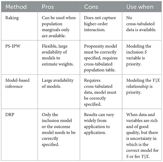
Table 1. Summary of adjustment methods pros and cons.

While non-probability samples pose significant challenges due to selection bias, they also offer valuable opportunities when handled with the right statistical methods. This paper has provided both an intuitive and technical overview of key approaches to adjust for bias and improve inference. Although no method can fully replace probability sampling, the techniques discussed here can enhance the reliability of estimates derived from non-representative data. By increasing awareness of both the risks and potential of these samples, this work aims to support researchers in making informed methodological choices when working with online and other non-probability datasets.

Author contributions

AA: Conceptualization, Data curation, Formal analysis, Investigation, Methodology, Software, Validation, Visualization, Writing – original draft, Writing – review & editing. MLT: Funding acquisition, Project administration, Supervision, Writing – original draft, Writing – review & editing. OP: Funding acquisition, Project administration, Supervision, Validation, Writing – original draft, Writing – review & editing.

Funding

The author(s) declare that financial support was received for the research and/or publication of this article. This work was part-funded by the PON “Research and Innovation” 2014–2020 Actions IV.4 “PhDs and research contracts on innovation issues” and Action IV.5 “PhDs on Green issues.” Ministerial Decree 1061/2021 as a PhD studentship to Alberto Arletti. Open Access funding provided by Università degli Studi di Padova | University of Padua, Open Science Committee The funders had no role in study design, data collection and analysis, decision to publish, or preparation of the manuscript.

Conflict of interest

The authors declare that the research was conducted in the absence of any commercial or financial relationships that could be construed as a potential conflict of interest.

Generative AI statement

The author(s) declare that Gen AI was used in the creation of this manuscript. Open AI GPT-4 is used to edit the manuscript, check grammar and spelling mistakes and latex formatting Open AI GPT-4.

Publisher's note

All claims expressed in this article are solely those of the authors and do not necessarily represent those of their affiliated organizations, or those of the publisher, the editors and the reviewers. Any product that may be evaluated in this article, or claim that may be made by its manufacturer, is not guaranteed or endorsed by the publisher.

References

Alexander, M., Polimis, K., and Zagheni, E. (2020). Combining social media and survey data to nowcast migrant stocks in the United States. Popul. Res. Policy Rev. 1–28. doi: 10.1007/s11113-020-09599-3