Association analysis between polygenic risk scores and traits: practical guidelines and tutorial with an illustrative data set of schizophrenia

Most methodological Polygenic Risk Score (PRS)-related papers explain the laborious process of computing the PRS in great depth. Afterwards, as a last step, it is generally described that to test a possible association between a PRS and a trait of interest, an analysis through regression models (linear or logistic, depending on data type) should be carried out adjusting for covariates (e.g., sex, age, clinical information, or genetic ancestry-based Principal Components). When covariates are included, measurements such as the increment on the variance explained by the addition of the PRS to the model or the significance of the PRS term are usually reported. However, the association study between PRSs and a trait is a complex concern that requires proper modeling and analysis, since interactions and validation conditions represent crucial aspects. Even though excellent papers explain how to use and interpret the results obtained with such regression models, sometimes important information from the previously calculated PRS may be lost, partly due to the automation of analyses. With this guide, we intend to fill a gap in association studies between PRSs and a trait and to facilitate the analysis, obtaining statistically correct results. It contains a motivating real data case analyzed exhaustively to illustrate how to face a real analysis. Besides, it is accompanied by four examples, called Working Examples, which present different situations the researcher may encounter along with the R code for analyzing all these data sets and the corresponding application of the steps in this guide.

1 Introduction

A Polygenic Risk Score (PRS) is an estimated value of an individual’s genetic susceptibility to a trait, condition, or disease, and it is calculated based on the results of a Genome-Wide Association Study (GWAS). Once it is calculated, a typical analysis includes testing for association between the PRS and a trait through a linear or logistic regression model. In the most common situation, the models include covariates such as sex, age, clinical diagnosis, or genetic ancestry-based Principal Components used to control for potential population substructure, among others. Then, to evaluate the effect of the PRS alone, two models are usually considered: the so-called null or baseline model and the full model. The null model consists of the trait as the response variable and the covariates as predictor variables. The full model incorporates the PRS into the null model as a predictor. They are nested models, usually with only one different term, the PRS. Then, both models are analyzed, and the significance of the PRS and the increase in the explained variance between the models are evaluated. Usually, the value of the coefficient of determination R², or the adjusted coefficient of determination, $R_{adj}^2$, is reported in the case of a continuous trait. Likewise, if it is a binary trait, the value of a pseudo-R² coefficient of Nagelkerke is reported.

There are different approaches to computing a PRS. The traditional Clumping + Thresholding (C+T) method enables the selection of independent variants through LD-pruning to avoid redundancy and the inclusion of more or less significantly associated variants with the discovery trait by establishing different GWAS p-value thresholds, often resulting in the generation of several PRSs according to the thresholds used (1). However, more advanced methods have been developed recently that re-weight the SNP effect sizes from the GWAS summary statistics, applying some form of shrinkage and usually allowing for obtaining a single PRS (2).

Although the literature includes excellent papers explaining how to use and interpret regression models (3–9), a guideline for conducting PRS association studies is necessary to assist non-statistician researchers in performing the statistical analyses correctly. Below are the guidelines for conducting these association analyses after calculating the PRS. Therefore, this guide does not focus on the calculation process used to obtain a PRS but rather on analyzing the association between a trait and a previously calculated PRS. This guide features a detailed real case to illustrate how to approach a real analysis. Additionally, it is accompanied by four examples, called Working Examples, which gradually present all the steps explained in increasing order of difficulty. Moreover, the data sets, R code for the analysis, and PDF files containing the results with software output are available at: https://github.com/ItziarI/SupportingMaterial-for-the-guide.

The definitions needed to follow the next sections are reported in Box 1. The different steps of the proposed guide are presented in the next section and summarized in Figure 1.

Figure 1

Figure 1. Workflow of the association analysis described in Section 2. Each panel is associated with one of the steps. Panel 1: describes the different possible models to consider, as explained in subsection 2.1; Panel 2: shows a plot related to subsection 2.2 where a semi-automated procedure to reduce the number of PRSs to be analyzed is presented; Panel 3: related to subsection 2.3 where it is discused how stablish the most appropiate model among all the possible ones; Panel 4: in this panel subsection 2.4 is summarized with the validation of the model and the different strategies to follow depending if the model is validated or not; Panel 5: shows the steps that should be followed for a correct analysis with a binary trait, as it is described in subsection 2.5.

Box 1. Definitions.
Null model: the trait is the response, and the covariates are the predictors.

Full model: the trait is the response; the PRS and covariates are the predictors.

Nested model: a regression model that includes only a subset of the predictor variables from the other regression model.

Coefficient of Determination R²: it gives the percentage variation in the response variable explained by the predictor variables. The range is 0 to 1 (i.e., 0% to 100% of the variation in the response can be explained by the predictor variables).

Adjusted Coefficient of Determination $R_{adj}^2$: it also indicates the goodness of the model, but adjusts for the number of predictors.

Pseudo-R² coefficient of Nagelkerke: similar to R² when the response variable is binary.

Akaike Information Criterion (AIC): metric used to compare the fit of different regression models. The model with the lowest AIC offers the best fit.

Discrimination coefficient D: measure of the discriminant capacity of the two-class logistic regression model. The range is between 0 and 1, with large values indicating the logistic model discriminates better between the classes.

Logit values: also known as “log-odds”, is the natural logarithm of the odds concerning one event. If p is the probability of an event, the odds is given by the ratio p/(1-p). The bigger this value, the greater the chances for the event to occur.

Validation of a linear regression model:

● Linearity: there is a linear relationship between each predictor and the response.

● Normality: the errors follow a normal distribution with a mean equal to zero

○ QQ-plot: short for “quantile-quantile” plot, is used to assess whether or not a set of data potentially came from some theoretical distribution.

○ Shapiro’s test: is used to determine whether or not a given dataset follows a normal distribution (H₀: data is normally distributed vs H₁: data is not normally distributed)

● Constant variance or homoscedasticity: constant variance for all subjects

○ Levene’s test: is used to determine whether or not the variance is constant

○ Heteroscedasticity: there is no homoscedasticity

Skewed data: if one tail is longer than the other, the distribution is skewed (or asymmetrical)

Nonparametric approach: a method that makes statistical inference without regard to any underlying distribution

Permutation test: permutation tests work by resampling the observed data many times to determine a p-value for the test

Box-Cox transformation: it is a useful family of transformations to convert a non-normal behaving data set into an approximately normal distribution.

Overdispersion: occurs when the discrepancies between the observed responses and their predictions according to the model are larger than what the binomial model would predict.

Binomial and quasi-binomial distribution: probability distributions that arise when counting the number of times an event of interest happens given a fixed number of trials. In the binomial distribution, the variance is completely determined by the probability of the event of interest. The quasi-binomial distribution has an extra parameter allowing additional variance compared to the binomial distribution.

2 Guidelines for the association analysis

2.1 Which full model should be considered?

The researcher should be aware of the possibility of different full models. In certain situations, it is necessary to consider models that incorporate interaction terms; however, only those interactions with biomedical meaning or interest for the researcher should be considered. Therefore, the number of models with interactions will not be large, as generally only those related to covariates such as sex, diagnosis, or age are considered. Therefore, for each PRS we can assume different full models. For instance, if there are two categorical covariates of interest, such as sex and diagnosis, four different full models (FM) can be considered (first panel in Figure 1):

● FM_WI: the model without interaction terms.

● FM_Sex: the model with the interaction term PRS×Sex.

● FM_Diag: the model with the interaction term PRS×Diag.

● FM_Sex/Diag: the model including the interaction terms PRS×Sex and PRS×Diag.

2.2 When and how to make a PRS ranking?

This section should only be considered if the researcher has used a PRS calculation method that has generated several PRSs to analyze (e.g., using several p-value thresholds in the C+T approach) and wants to determine which of these PRSs are of greatest interest before performing the association analysis to avoid having to analyze all of them. Instead, if the method generates only a single PRS, this step should be skipped, and the next step is in subsection 2.3.

We propose a semi-automated procedure to reduce the number of PRSs that need detailed analysis. If the trait is continuous, for each PRS and each possible full model (including and excluding interaction terms), calculate the coefficient of determination R² and let S be the sum of all of them. Similarly, if the trait is binary, calculate the pseudo-R² coefficient of Nagelkerke or the discrimination coefficient D for each full model and the sum S of these values. Next, rank the PRSs by S in decreasing order. This ranking is generated automatically, and the top PRSs, which explain more phenotypic variance across all full models, deserve a more careful analysis. Note that this sum incorporates information from all considered models and its use prevents the need to rank all possible models across different PRSs.

The PRSs should be analyzed individually, following the ranking established by S until no association is found for a given PRS. The possible gap in the S values between two consecutive PRSs can also be used as a stopping rule.

A visualization of this PRS rank is possible, as shown in panel 2 of Figure 1. The x-axis represents the S values, and vertical lines can be drawn at different points, such as the mean, median, or percentiles of S. Each horizontal line represents a PRS. Black dots symbolize the S value for each PRS, and adjacent whiskers represent the standard deviation of the R² values (pseudo-R² coefficient of Nagelkerke or the discrimination coefficient D, respectively) obtained from all possible full models. Thus, the length of these horizontal bars can be interpreted as an indicator of the importance of considering interactions between a PRS and the covariates.

2.3 Which model among all the possible ones is the most appropriate?

For a fixed PRS, it is necessary to determine which is the most appropriate full model. First, it must be determined if the model should contain interaction terms, and if so, which ones.

For a continuous trait, scatterplots of the trait and PRS by categorical predictors are useful for visually checking the homogeneity of slopes and determining whether interaction terms should be included. For example, panel 3 of Figure 1 contains four scatterplots, each showing the relationship between a trait and PRS.4, separated by sex and diagnosis. Different slopes are observed. For diagnosis 1, the slopes increase (for both sexes 0 and 1); whereas for diagnosis 0, the slopes are very gentle, either slightly increasing (sex = 0) or slightly decreasing (sex = 1). Therefore, the interaction term “PRS×Diagnosis” should be included in the full model.

For a binary trait, compute the model with all possible interactions and plot the predicted logit values against the PRS. If interaction terms are relevant, different logit behaviors should appear.

At this point, a full model candidate is established; it is crucial to verify whether it meets the conditions required by the statistical analysis, as explained below. However, this validation is not typically performed in automated analyses.

2.4 For a continuous trait, what steps should be followed for a correct analysis?

If the outcome variable is a continuous trait, the focus must be placed on different issues (panel 4 in Figure 1).

2.4.1 How is the candidate model validated?

To validate the full model for a continuous trait, linearity (by scatter plots of trait and PRS), normality (by QQ-plots and Shapiro’s test), and constant variance or homoscedasticity (by Levene’s test) must be checked. The fourth validity condition, the independence of the observations, is generally guaranteed by the design of the experiment itself. Remember that the analysis does not assume normality for either the predictors or the trait. The assumption is that errors are normally distributed, with a mean of zero. The verification of these conditions is relevant in the context of inference regarding the interpretability and significance of the coefficients. For instance, heteroscedasticity tends to produce smaller p-values than they should be (10). Consequently, this problem can lead to the conclusion that a model term is statistically significant when it is not. Furthermore, heteroscedasticity persists as a problem, regardless of sample size.

2.4.2 What can be done if any validation condition fails?

Different strategies will be considered depending on the failed validation condition (panel 4.2 in Figure 1).

When it is suspected that the normality of errors fails, but the model is homoscedastic, and the linearity is maintained, try transforming the response variable. For instance, take the logarithm for positively skewed data or the square root for more moderate skewness situations. Such a transformation aims to rebuild a valid candidate model that allows for assessing the association between the PRS and the trait. However, a nonparametric approach is also possible. A permutation test allows researchers to measure whether the increase in the determination coefficient observed between the null model and the candidate full model is significant. However, with this type of nonparametric approach, it will not be possible to establish if the association is significant or how the variation (of one unit) of the PRS affects the trait. Furthermore, it will not be possible to evaluate the different behavior of the PRS in the groups generated by the categorical variable.

If heteroscedasticity is suspected but the linearity of the model is maintained, it would be advisable to try a Box-Cox transformation of the response variable. The Box-Cox transformations for different values of λ are given by: (trait – 1)/λ, if λ ≠ 0, and log(trait) if λ = 0. Again, it is possible to consider a nonparametric approach. Now, use a weighted permutation test to measure whether the increase in the determination coefficient observed between the null and the selected full model is significant. During its construction process, the weighted permutation test considers heteroscedasticity, making the underlying residuals interchangeable.

If the problem lies in the linearity, try a transformation of the response variable or include new non-linear terms.

2.4.3 How is a possible association established?

Once the PRS, the model, and its validation have been established, analyze the possible association by checking the value and significance of the regression coefficients. At this point, great care must be taken when interpreting the lists provided by the most common software. This is extremely important if the model contains interaction terms, as the value of the PRS coefficient and its significance can vary depending on the group to which each individual belongs.

The detailed Working Examples 1-3, included in the Supporting material (see Section 8), aim to understand the necessity of performing these steps and how to perform them correctly (Working Example 1: Continuous trait, and model fulfilling all assumptions; Working Example 2: Continuous trait and steps taken to address the non-normality of errors; Working Example 3: Continuous trait and the steps taken to address issues in the initial fitted model with non-constant variance.)

2.5 For a binary trait, what steps should be followed for a correct analysis?

If the outcome variable is a binary trait, given a PRS, check overdispersion once the full model has been established. When the ratio comparing the residual deviance with the degrees of freedom is considerably larger than 1, the assumption of binomial variation is violated, and then overdispersion occurs. Overdispersion can also be checked by fitting a logistic regression under two different models using a binomial and a quasi-binomial distribution, respectively. If there is statistical evidence that the expected variance of the two models is significantly different, we can conclude that there is overdispersion. If the candidate full model has no overdispersion, check the significance of the PRS, and analyze the possible association with the trait.

On the contrary, if overdispersion is detected (panel 5 in Figure 1), a simple solution to overdispersion would be to estimate an additional parameter that indicates the amount of overdispersion and specify a quasi-binomial family instead of a binomial in the logistic regression model. Again, when the model includes interaction terms, it is crucial to interpret correctly possible significant associations (see the detailed explanations in Working Example 4).

When working with binary traits, it is also possible to use a nonparametric approach by a permutation test to assess whether the increase in the pseudo-R² coefficient of Nagelkerke or the coefficient of discrimination D is significant. However, the limitations of this approach must be kept in mind, as it will not be possible to determine regression coefficients or their significance.

2.6 Is it necessary to consider all the steps mentioned above?

The answer is Yes. Not considering interaction terms may mask associations between PRS and trait in some groups determined by the corresponding categorical covariate. Ignoring model validation can lead to negative consequences, such as mistakenly concluding that the PRS is significantly associated with the trait when it isn’t. The Working Examples and the real data set demonstrate how poor analysis leads to erroneous conclusions. Finally, the real data set illustrates the difficulties that can arise with real data and how they can be solved following this guide, for both continuous and binary traits.

3 Analysing a real data set

The real data set contains a PRS for psychotic-like experiences (PLEs) computed for 227 healthy individuals, including 64 men (28.1%) and 164 women (71.9%). PLEs are similar to psychotic experiences to those experienced by patients with schizophrenia, but are found in an attenuated form in healthy subjects. PLEs are considered to be normally distributed in the general population, with just a few individuals presenting high levels of PLEs and thus being the ones at risk of developing psychosis (11–13). The PRS in this example was calculated based on the latest GWAS on PLEs (14) with the classical Clumping + Thresholding method (1), using 106 p-value thresholds ranging from 5×10⁻⁸ to 1 to allow us to exemplify the second step of this guide. This motivational example aims to determine which PRSs for PLEs (PLE-PRSs) are associated with a phenotypic measure of PLEs in non-clinical individuals.

Specifically, participants in this data set completed the Community Assessment of Psychic Experiences (CAPE) questionnaire (15), which assesses three dimensions of PLEs: positive, negative, and depressive dimensions. For this tutorial, we used the information on the positive and negative dimensions of PLEs (CAPE Positive and CAPE Negative, respectively).

We considered CAPE Negative as a continuous trait and CAPE Positive as a binary trait separating individuals with high and low levels of PLEs to illustrate how to apply the steps of this guide for both linear and logistic regression models, respectively. In both situations, sex, age, and the first two ancestry-based Principal Components are used as covariates. A larger number of PCs have not been included as usual since it would not add meaningful insight for our purpose and would only lengthen the results tables. The descriptive characteristics of this real data set are in Table 1.

Table 1

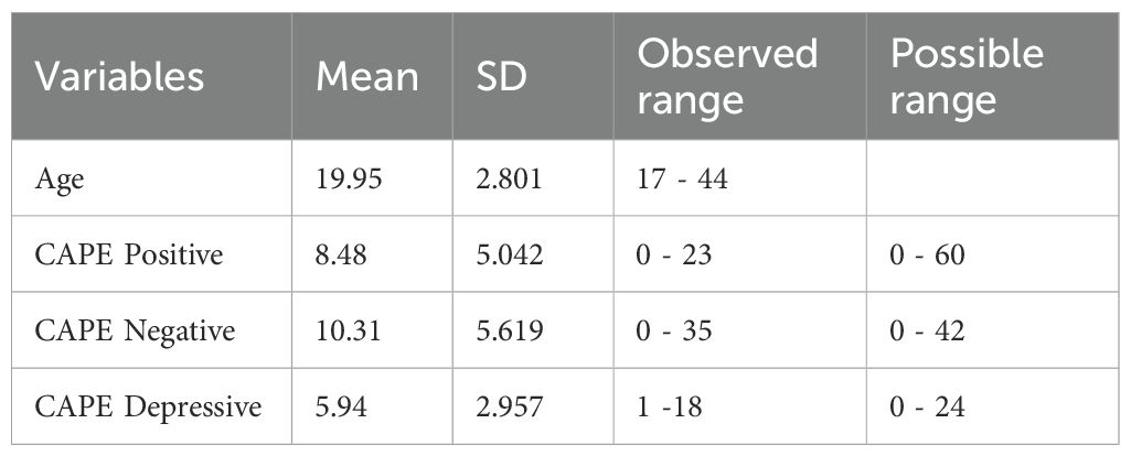
Table 1. Descriptive characteristics of the real data set.

The question is: out of the 106 PRSs that were built, which are the most important to carry out a detailed association analysis? Furthermore, does it make sense to consider models that include interaction terms, for example, between PRS and sex or between PRS and age? Note that if these interaction terms are included and they are significant, we will obtain information regarding how the increase/decrease in PRS values affects the Positive CAPE or Negative CAPE values depending on whether the individual is male (coded by 0) or female (coded by 1), or depending on their age. This information will be lost if interactions are not introduced into the model.

For a better understanding of the results detailed below, it is recommended to run the scripts (see Section 8) simultaneously.

3.1 CAPE negative as the trait

Considering the biomedical meaning of the analysis, only the full models FM_WI (without interaction terms) and FM_Sex (including the interaction term PRS×Sex) are considered. For each model, we calculated the coefficient of determination R² and the sum $S = R_{WI}^2 + R_{Sex}^2$. We ranked the PRSs, and we identified PRS.13 (i.e., the PRS derived from GWAS p-value threshold = 0.07) as the top-ranked. Note that if the method used to compute the PLE-PRSs had been one that generates a single PRS, this step would have been omitted.

For PRS.13, the first of the PRSs rank, the short length of the horizontal bars in Figure 2, and the scatter plots of Trait vs. PRS.13 according to sex (Figure 3), which was the only categorical predictor, indicated the lack of interaction. Thus, we considered the following model, FM_WI: CAPE_Neg versus PRS.13 + Sex + Age + PC1 + PC2, as a candidate full model.

Figure 2

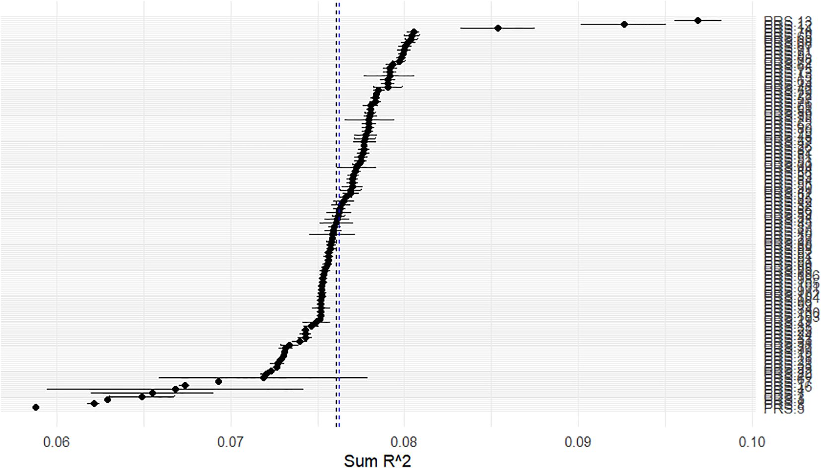
Figure 2. Real data set. On the x-axis, the S values described in section 2.2 are plotted. On the y-axis, the PRSs are ranked in decreasing order according to S. Black dots represent the S for each PRS, and the adjacent whiskers represent the standard deviation of the R² values obtained for the possible full models (including and not including interaction terms).

Figure 3

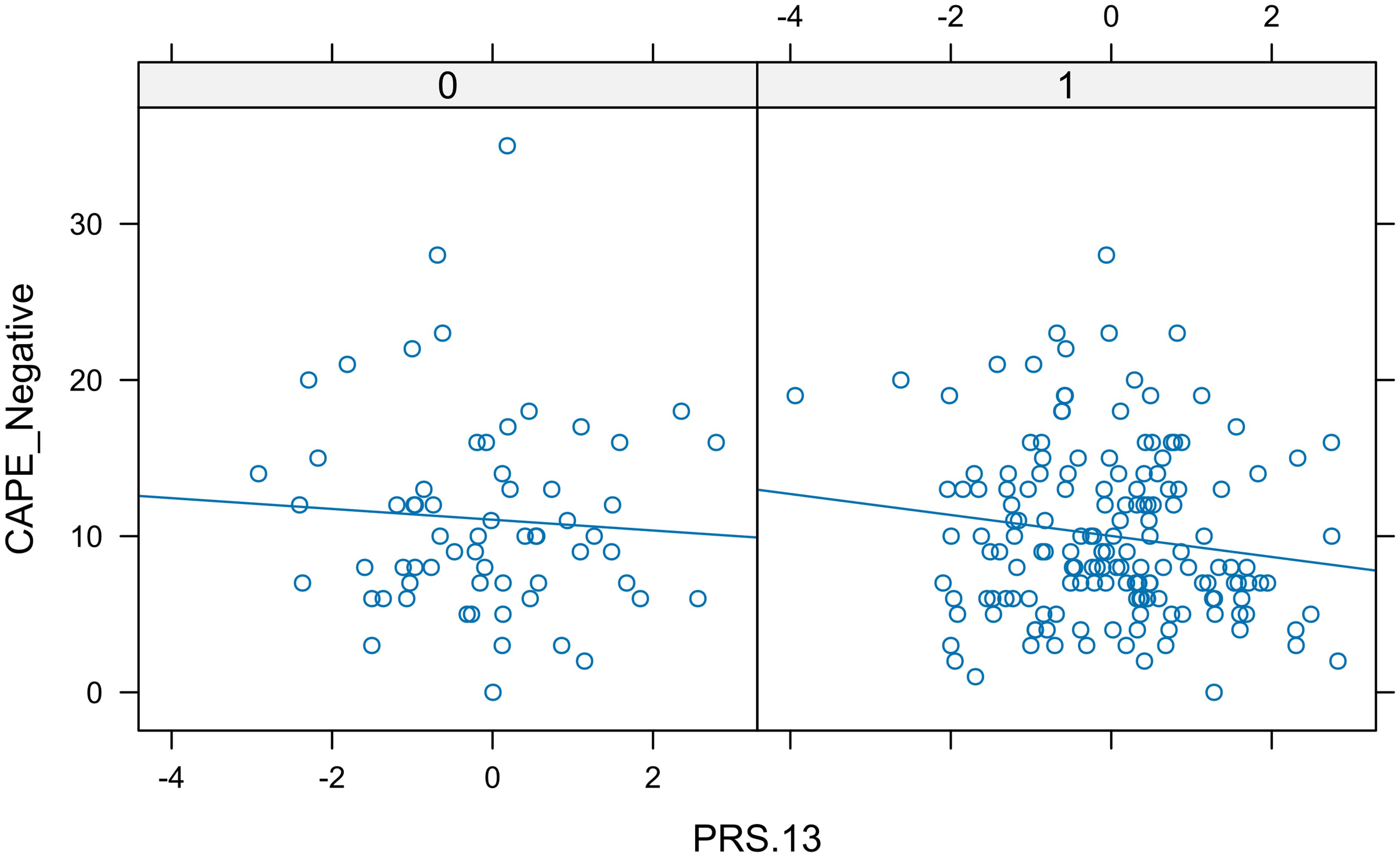
Figure 3. Real data set. In each panel, a scatter plot showing the relationship between negative CAPE and PRS.13 separated by sex. The similar slope of the lines indicated the lack of interaction.

The residuals did not follow a normal distribution (Shapiro test p-value = 4.335e-06; see Figure 4a), so a square root transformation was applied. With this transformation, the normality condition is already met (Shapiro test p-value = 0.0811), and the homoscedasticity assumption also holds (Levene’s test p-value = 0.5846; Figure 4b). The results showed that PRS.13 was significantly (p-value = 0.045) related to the sqrt(CAPE_Neg) in the following way:

Figure 4

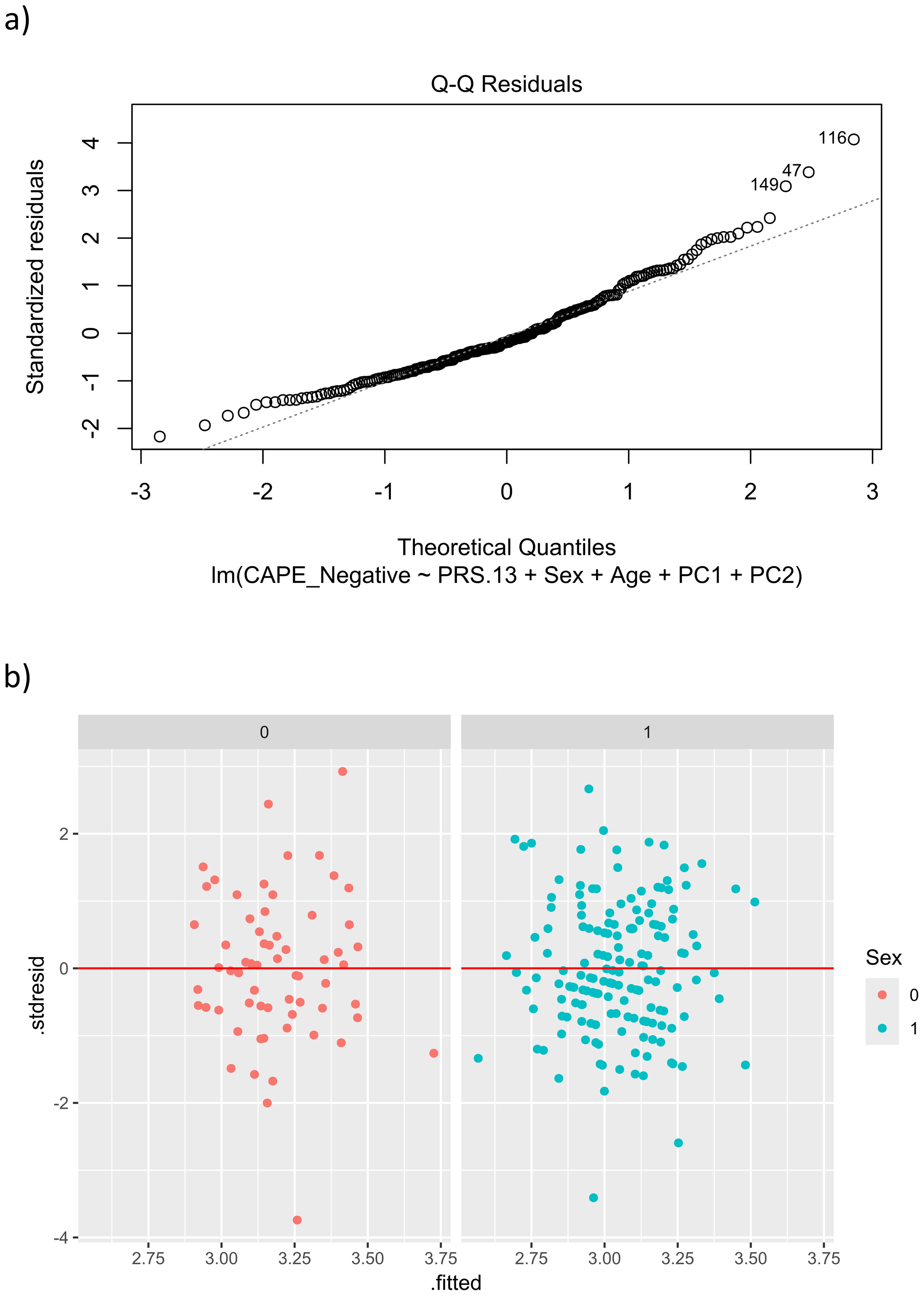
Figure 4. Real data set. Validation conditions for the model FM_WI: CAPE_Neg versus PRS.13 + Sex + Age + PC1 + PC2. (a) QQ-plot for normality, deviations from the diagonal line indicate that the errors’ distribution differs from a normal distribution. (b) Plot for homocedasticity after squared root transformation, each panel shows the scatter plot of residuals versus fitted values according to sex.

$$\begin{array}{c}\widehat{\sqrt{\text{CAPE}\_\text{Neg}}}=3.013-0.101·PRS.13-0.142·Sex+0.009\\ ·Age+3.797·PC1+8.409·PC2\end{array}$$

and then,

$$\begin{array}{c}\widehat{\text{CAPE}\_\text{Neg}}=(3.013-0.101·PRS.13-0.142\\ ·\text{S}ex+0.009·Age+3.797·PC1+8.409·PC2{)}^2\end{array}$$

The effect of the change of one unit in PRS.13 in CAPE_Neg can be measured as follows. Compute the estimations at the indicated values of PRS.13

$$\widehat{(\text{CAPE}\_{\text{Neg}}_0}) \text{and PRS }.13+\mathrm{1 }\widehat{(\text{CAPE}\_{\text{Neg}}_1}):$$

$$\begin{array}{c}\widehat{\text{CAPE}\_{\text{Neg}}_0}=(3.013-0.101·PRS.13-0.142\\ ·\text{S}ex+0.009·Age+3.797·PC1+8.409·PC2{)}^2\end{array}$$

and

$$\begin{array}{c}\widehat{{\text{CAPE}}_{{\text{Neg}}_1}}=(3.013-0.101·(PRS.13+1)-0.142·\text{S}ex+0.009\\ ·Age+3.797·PC1+8.409·PC2{)}^2={(-0.101+\sqrt{\widehat{\text{CAPE}\_{\text{Neg}}_0}})}^2\end{array}$$

then, difference

$$\widehat{\text{CAPE}\_{\text{Neg}}_1}-\widehat{\text{CAPE}\_{\text{Neg}}_0}$$

is given by:

$${(-0.101)}^2+2·(-0.101)·\sqrt{\widehat{\text{CAPE}\_{\text{Neg}}_0}}$$

Thus, if the current CAPE_Neg is, for instance, 5, 10, or 25, increasing one unit in PRS.13 is associated with a change of $-0.4415, -0.6286, \text{and}-0.9998$ in CAPE_Neg, respectively.

With the permutation test, we obtained a significant (p-value = 0.0033) increase of 0.0197 in the coefficient of determination when the PRS.13 was included in the baseline model.

The next PRS in the ordered list was PRS.12, and Figure 5 indicated that the interaction term should be considered. Again, the residuals did not follow a normal distribution, and neither with a transformation nor using the permutation test, a significant association was found between PRS.12 and CAPE_Neg (p-value = 0.7170 and 0.0956, respectively). Therefore, there is no need to study more candidate PRSs.

Figure 5

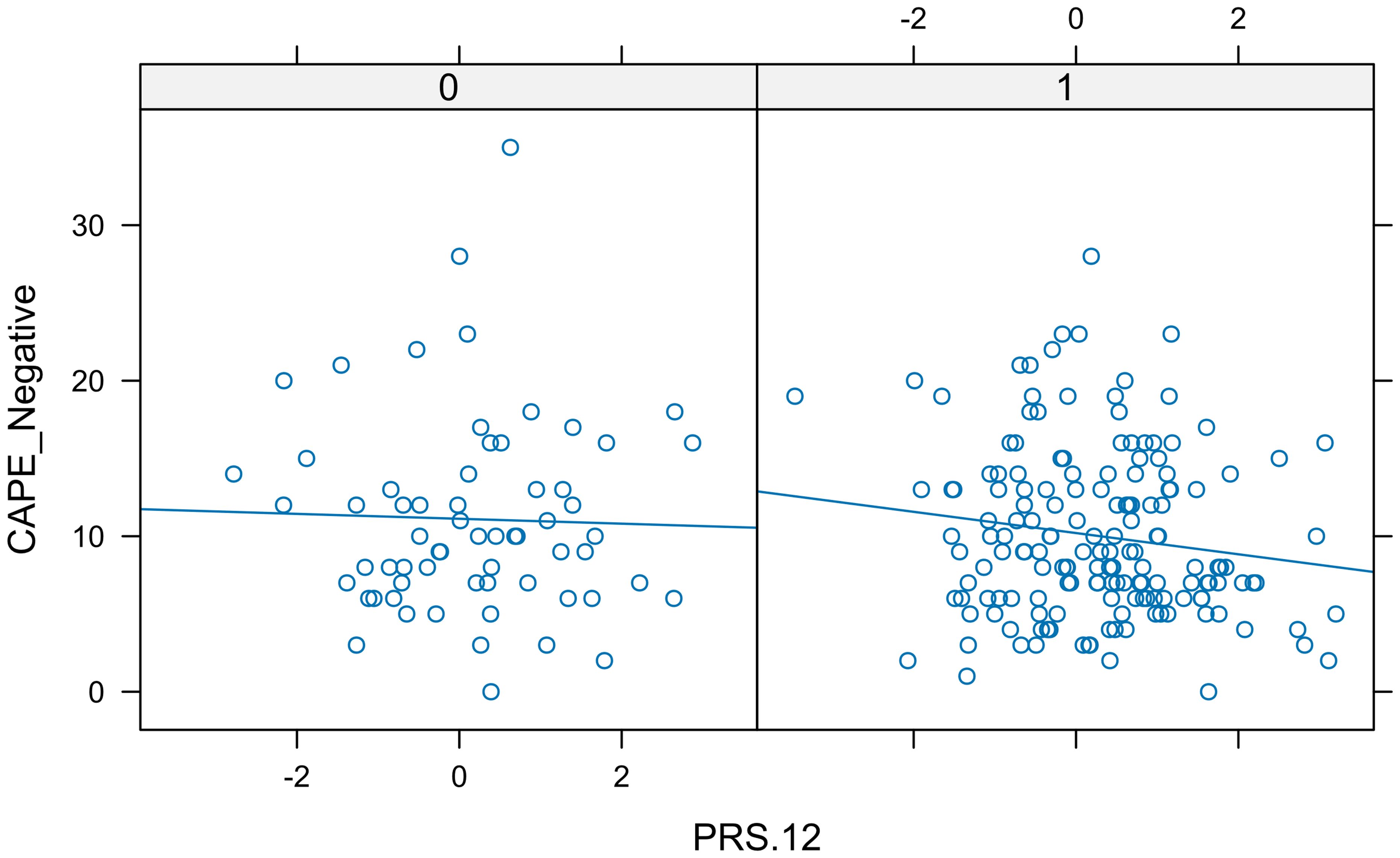
Figure 5. Real data set. In each panel, a scatter plot shows the relationship between CAPE negative and PRS.12 separated by sex. The different slopes of the lines indicated the presence of interaction.

3.2 CAPE positive as the trait

Finally, we considered CAPE Positive as a binary trait separating individuals with high and low levels of PLEs. This scale has no fixed criterion to decide who scores high and who scores low. However, based on its histogram, we considered a threshold of 15 to indicate those individuals who would score high (the 1% of the sample). According to the discrimination coefficient D, the top PRS was PRS.15 (i.e., the PRS derived from GWAS p-value threshold = 0.09). The plot of the predicted logit values against the PRS.15 indicated that the interaction term was relevant (Figure 6).

Figure 6

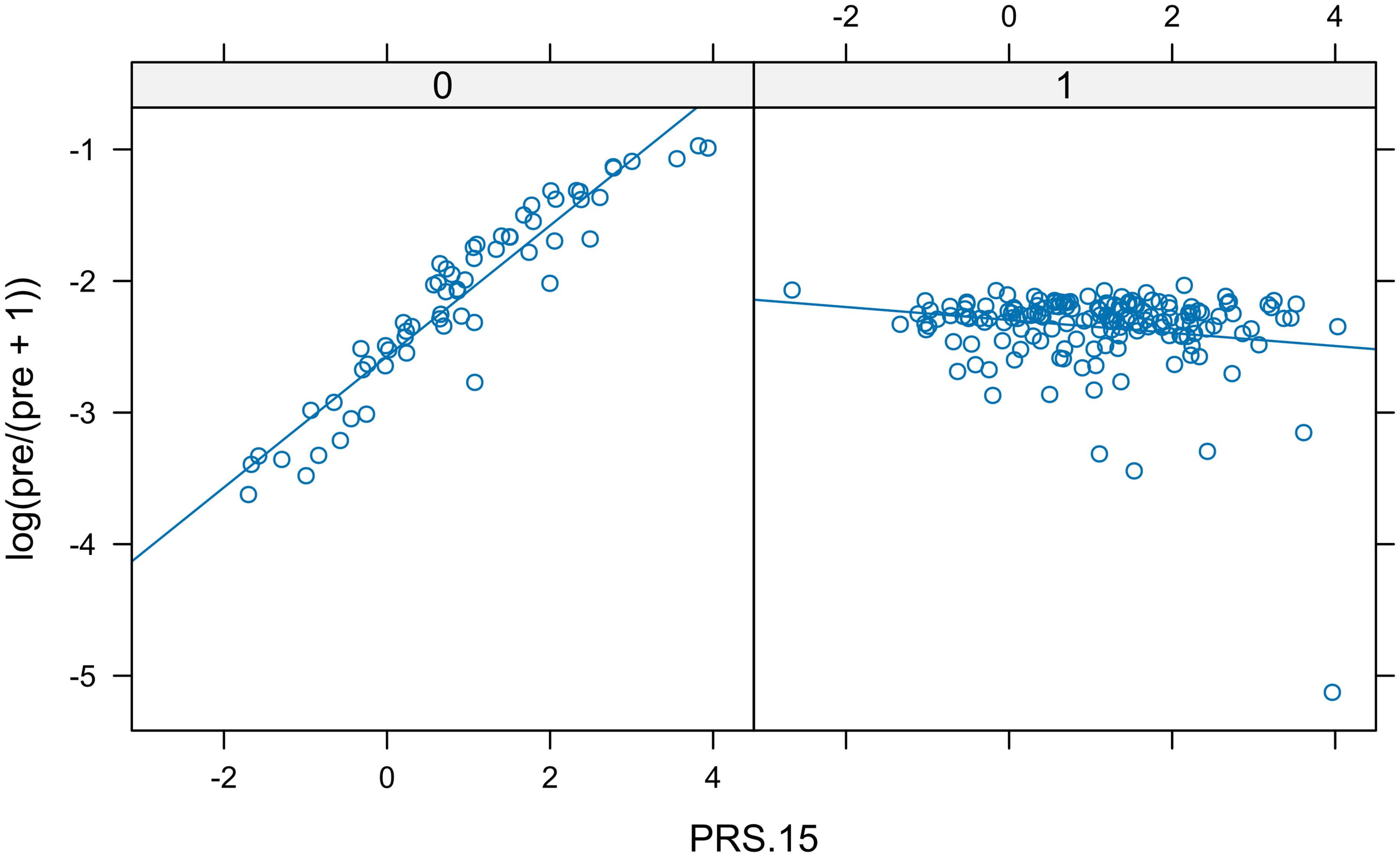
Figure 6. Real data set. In each panel, a scatter plot of fitted logit predictions shows the relationship between positive CAPE and PRS.15 separated by sex. The different slopes of the lines indicated the presence of interaction.

As overdispersion was not detected (p-value = 0.2651), we analyzed the possible association with CAPE_Pos. Note that in Table 2 (standard output given by the R package), values associated with PRS.15 for Sex=0 are in the second line (coefficient b₁). Those for Sex=1 are, for the intercept, in lines 1 and 3 (coefficients b₀ and b₃); for the PRS.15 coefficient in lines 2 and 7 (coefficients b₂ and b₆). Thus, the PRS.15 coefficient that varies depending on the sex (Table 2), is given by:

Table 2

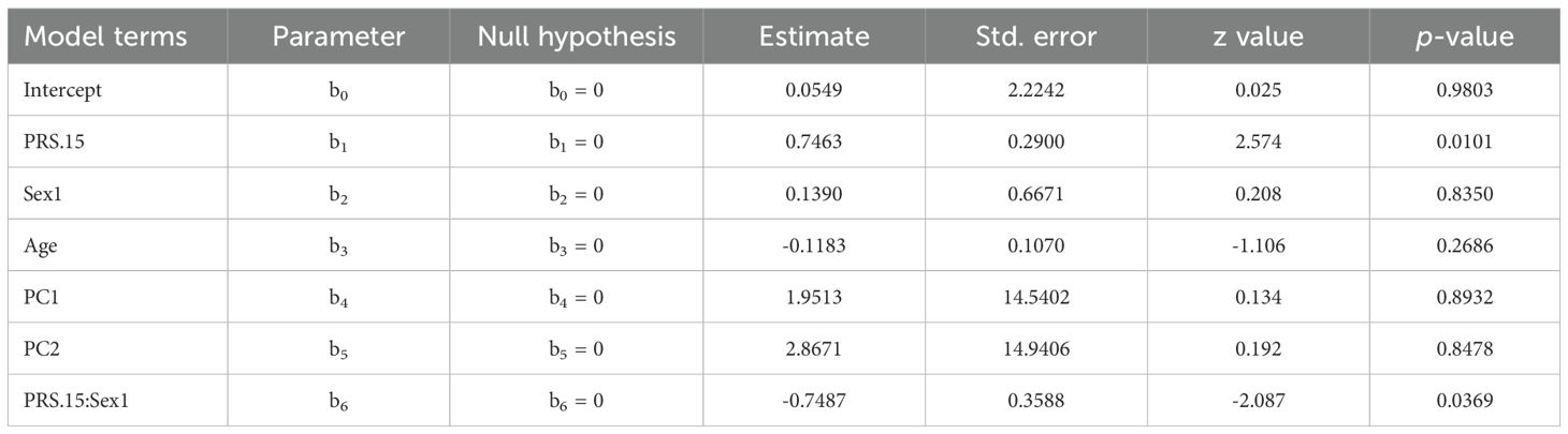
Table 2. For the real data set with a binary Trait, logistic regression results for CAPE Positive versus PRS.15, considering interaction with Sex.

● If Sex = 0,

$$\begin{array}{c}\widehat{\text{log}(\frac{p}{1-p})}=0.055+0.746·\text{PRS}.15-0.118\\ ·\text{Age}+1.951·\text{PC}1+2.867·\text{PC}2\end{array}$$

● If Sex = 1,

$$\begin{array}{c}\widehat{\text{log}(\frac{p}{1-p})}=(0.055+0.139)+(0.746-0.749)·\text{PRS}.15-0.118\\ ·\text{Age}+1.951·\text{PC}1+2.867·\text{PC}2\end{array}$$

That means that for those with Sex=1, the PRS.15 is not related (p-value = 0.9910) to CAPE_Pos with odds = exp($-$ 0.002) = 0.998. For those with Sex = 0, the model indicates that PRS.15 is significantly associated (p-value = 0.0101) with the CAPE_Pos with a coefficient 0.7463, so the odds increase exp(0.7463) = 2.109 for an incremental of one unit in PRS.15 (see Table 3). It is very important to note that if the interaction is not included in the model, meaning that if the model assumes the association of PRS.15 to be the same for both sex categories, then the association of PRS.15 with CAPE_Pos might be lost (p-value = 0.0764). Most importantly, the different behavior regarding sex would not have been detected.

Table 3

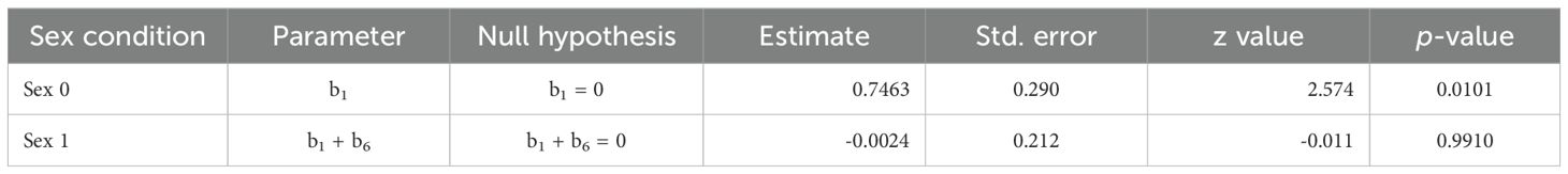
Table 3. For the real data set with a binary Trait, and according to sex, parameters, null hypothesis, estimates, standard errors, z statistics, and p-values using model FM_Sex.

The analysis continued, studying the possible association with the following PRS from the list obtained. For the first six ranked PRSs, Table 4 shows a clear association with CAPE_Pos in group Sex equal to 0, but not when Sex is 1. Note that all these associations would have been lost if the interaction term had not been considered.

Table 4

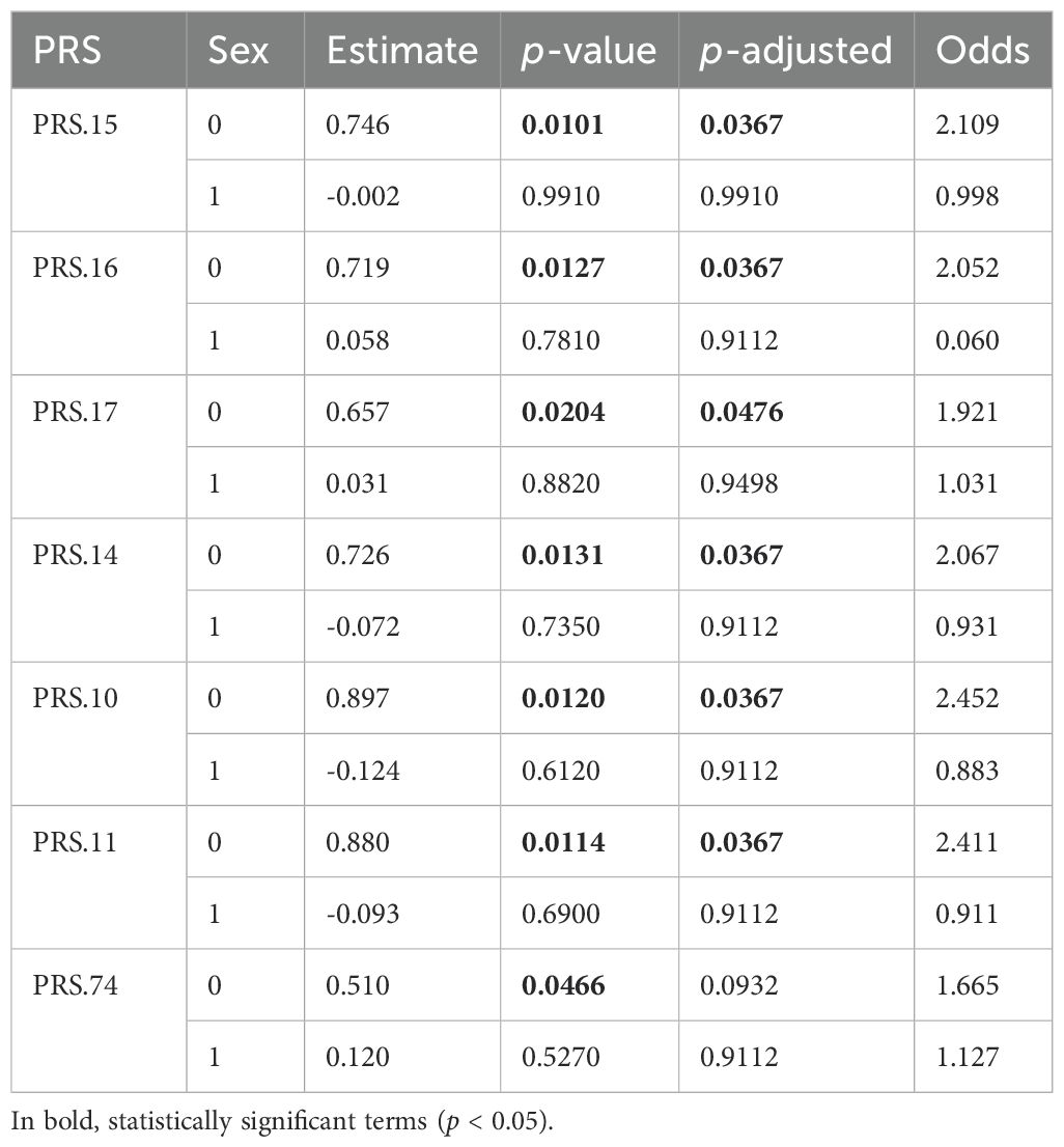
Table 4. For the real data set with a binary Trait and according to sex, estimates, p-values, and odds using model FM_Sex

4 Concluding remarks

This paper presents a guide based on simple steps to help researchers in PRS studies. We describe these steps and present different situations and solutions through Working Examples and with a real data set. The situations presented in this guide do not cover all possible scenarios. For this reason, we have prioritized the most common ones. In our opinion, this is not about showing all possible options, but rather highlighting the need for a more detailed study for some (not all) PRS that appear as prioritized candidates with a possible association with the trait. In this work, we have not considered the case of having a categorical trait with more than two categories. Since it is a situation of great interest, we will give the attention it deserves in future work. Finally, this guide is focused on the analysis of the association of a PRS with a trait, and it does not delve into which methodology is the most appropriate or up-to-date for calculating the PRS. Nevertheless, it is important to recognize that each step in the process, from GWAS discovery to PRS calculation and the subsequent association analyses, introduces potential sources of error (e.g., limited GWAS power, imputational inaccuracies, or suboptimal PRS parameter choices), and the accumulation of these can influence the robustness and interpretation of the final results (16). Furthermore, it should not be forgotten that the accuracy of a PRS depends on the genetic ancestry of the group used to obtain it, and that it may present significantly lower accuracy when applied to other groups (17, 18). Finally, it does not detail the concepts or statistical techniques it encourages to use, since it only aims to indicate which steps should be followed to perform a correct analysis.

Data availability statement

The datasets presented in this study can be found in online repositories. The names of the repository/repositories and accession number(s) can be found below: https://github.com/ItziarI/SupportingMaterial-for-the-guide.

All data sets, R code for the analysis, PDF files containing the analyses with the software, outputs for the Working Examples, and the real data sets can be found at https://github.com/ItziarI/SupportingMaterial-for-the-guide.

Ethics statement

Ethical approval was obtained from local research ethics committees. Written informed consent to participate in this study was was obtained from all participants in accordance with the national legislation and the institutional requirements.

Author contributions

II: Writing – original draft, Conceptualization, Software, Writing – review & editing, Methodology, Validation, Supervision, Formal Analysis, Data curation. PM-B: Supervision, Data curation, Writing – review & editing. SP: Supervision, Writing – review & editing. NB-V: Writing – review & editing, Supervision. AR: Supervision, Data curation, Writing – review & editing. CA: Supervision, Data curation, Software, Conceptualization, Writing – review & editing, Writing – original draft, Methodology, Formal Analysis, Validation.

Funding

The author(s) declare financial support was received for the research and/or publication of this article. This research was partially supported: II by the Spanish ‘Ministerio de Economia y Competitividad’ (PID2021-122402OB-C21 and PID2019-106942RB-C31). CA by the Spanish ‘Ministerio de Economia y Competitividad’ (PID2021-122402OB-C21 and PID2021-127776OB-I00) and by the project 2021SGR01421 (Generalitat de Catalunya). PM-B, NB-V and AR by the Spanish Ministry of Economy and Competitiveness (PSI2017-87512-C2-01 and 02-R; PID2020-119211RB-I00) and the projects 2021SGR00706 and 2021SGR01010 (Generalitat de Catalunya). PM-B was further funded by the PhD scholarship program FI-SDUR (2021-FISDU-00032) from Agencia de Gestión de Ayudas Universitarias y de Investigación (AGAUR).

Conflict of interest

The authors declare that the research was conducted in the absence of any commercial or financial relationships that could be construed as a potential conflict of interest.

The author(s) declared that they were an editorial board member of Frontiers, at the time of submission. This had no impact on the peer review process and the final decision.

Generative AI statement

The author(s) declare that no Generative AI was used in the creation of this manuscript.

Any alternative text (alt text) provided alongside figures in this article has been generated by Frontiers with the support of artificial intelligence and reasonable efforts have been made to ensure accuracy, including review by the authors wherever possible. If you identify any issues, please contact us.

Publisher’s note

All claims expressed in this article are solely those of the authors and do not necessarily represent those of their affiliated organizations, or those of the publisher, the editors and the reviewers. Any product that may be evaluated in this article, or claim that may be made by its manufacturer, is not guaranteed or endorsed by the publisher.

References

1. Choi SW, Mak TS, and O’Reilly PF. Tutorial, a guide to performing polygenic risk score analyses. Nat Protoc. (2020) 15:2759–72. doi: 10.1038/s41596-020-0353-1, PMID: 32709988

PubMed Abstract | Crossref Full Text | Google Scholar

2. Allegrini AG, Baldwin JR, Barkhuizen W, and Pingault JB. Research Review: A guide to computing and implementing polygenic scores in developmental research. J Child Psychol Psychiatry. (2022) 63:1111–24. doi: 10.1111/jcpp.13611, PMID: 35354222

PubMed Abstract | Crossref Full Text | Google Scholar

3. Altman N and Krzywinski M. Simple linear regression. Nat Methods. (2015) 12:999–1000. doi: 10.1038/nmeth.3627, PMID: 26824102

PubMed Abstract | Crossref Full Text | Google Scholar

4. Krzywinski M and Altman N. Multiple linear regression. Nat Methods. (2015) 12:1103–4. doi: 10.1038/nmeth.3665, PMID: 26962577

PubMed Abstract | Crossref Full Text | Google Scholar

5. Altman N and Krzywinski M. Analyzing outliers: influential or nuisance? Nat Methods. (2016) 13:281–2. doi: 10.1038/nmeth.3812, PMID: 27482566

PubMed Abstract | Crossref Full Text | Google Scholar

6. Altman N and Krzywinski M. Regression diagnostics. Nat Methods. (2016) 13:385–6. doi: 10.1038/nmeth.3854

Crossref Full Text | Google Scholar

7. Bzovsky S, Phillips MR, and Guymer RH. The clinician’s guide to interpreting a regression analysis. Eye. (2022) 36:1715–7. doi: 10.1038/s41433-022-01949-z, PMID: 35102247

PubMed Abstract | Crossref Full Text | Google Scholar

8. Lever J, Krzywinski M, and Altman N. Logistic regression. Nat Methods. (2016) 13:541–2. doi: 10.1038/nmeth.3904

Crossref Full Text | Google Scholar

9. Lever J, Krzywinski M, and Altman N. Model selection and overfitting. Nat Methods. (2016) 13:703–4. doi: 10.1038/nmeth.3968

Crossref Full Text | Google Scholar

10. Frost J. Regression Analysis: An Intuitive Guide for Using and Interpreting Linear Models. State College, PA, USA: Statistics by Jim Publishing (2020).

Google Scholar

11. Barrantes-Vidal N, Grant P, and Kwapil TR. The role of schizotypy in the study of the etiology of schizophrenia spectrum disorders. Schizophr. Bull. (2015) 41:S408–16. doi: 10.1093/schbul/sbu191, PMID: 25810055

PubMed Abstract | Crossref Full Text | Google Scholar

12. Guloksuz S and van Os J. The slow death of the concept of schizophrenia and the painful birth of the psychosis spectrum. Psychol Med. (2018) 48:229–44. doi: 10.1017/S0033291717001775, PMID: 28689498

PubMed Abstract | Crossref Full Text | Google Scholar

13. Guloksuz S and van Os J. En attendant godot: waiting for the funeral of “Schizophrenia” and the baby shower of the psychosis spectrum. Front Psychiatry. (2021) 12:618842. doi: 10.3389/fpsyt.2021.618842, PMID: 34122159

PubMed Abstract | Crossref Full Text | Google Scholar

14. Legge SE, Jones HJ, Kendall KM, Pardiñas AF, Menzies G, Bracher-Smith M, et al. Association of Genetic Liability to Psychotic Experiences with neuropsychotic disorders and traits. JAMA Psychiatry. (2019) . 76:1256–65. doi: 10.1001/jamapsychiatry.2019.2508, PMID: 31553412

PubMed Abstract | Crossref Full Text | Google Scholar

15. Konings M, Bak M, Hanssen M, and Krabbendam L. Validity and reliability of the CAPE, a self-report instrument for the measurement of psychotic experiences in the general population. Acta Psychiatr Scand. (2006) 114:55–61. doi: 10.1111/j.1600-0447.2005.00741.x, PMID: 16774662

PubMed Abstract | Crossref Full Text | Google Scholar

16. Stein C, Asgari S, Gonzaga-Jauregui C, Landstrom A, Lemke A, Li J, et al. Addressing the challenges of polygenic scores in human genetic research. Am J Hum Genet. (2022) 109:2095–100. doi: 10.1016/j.ajhg.2022.10.012, PMID: 36459976

PubMed Abstract | Crossref Full Text | Google Scholar

17. Peterson RE, Kuchenbaecker K, Walters RK, Chen CY, Popejoy AB, Periyasamy S, et al. Genome-wide association studies in ancestrally diverse populations: opportunities, methods, pitfalls, and recommendations. Cell. (2019) 179:589–603. doi: 10.1016/j.cell.2019.08.05118, PMID: 31607513

PubMed Abstract | Crossref Full Text | Google Scholar

18. Duncan L, Shen H, Gelaye B, Meijsen J, Ressler K, Feldman M, et al. Analysis of polygenic risk score usage and performance in diverse human populations. Nat Commun. (2019) 10:3328. doi: 10.1038/s41467-019-11112-0, PMID: 31346163

PubMed Abstract | Crossref Full Text | Google Scholar