Machine learning pipeline for microparticle size classification in self-mixing interferometric signals for flow cytometry

Self-mixing interferometry (SMI) is an emerging optical sensing technique for detecting and classifying microparticles in non-contact and label-free flowmetry applications. High precision and reliability are essential for its integration into medical diagnostics, such as blood analysis, and quality control in chemical manufacturing processes. While theoretical models describe SMI-induced signal modulations caused by particle passage, challenges persist due to signal noise, variability, and interpretability under experimental conditions. This study enhances SMI-based particle size classification by integrating machine learning (ML) models to improve feature extraction and classification accuracy. Three ML pipelines are evaluated, achieving 98% classification accuracy in distinguishing particles of different sizes (2, 4, and 10 µm). The high classification accuracy demonstrates the scalability of our approach, ensuring its applicability across diverse particle analysis scenarios.

1 Introduction

Self-mixing interferometry (SMI), also known as optical feedback interferometry (OFI), has gained significant attention due to its versatility and cost-effectiveness in sensing applications (Perchoux et al., 2016; Donati and Norgia, 2014; Quotb et al., 2021; Taimre et al., 2015). This laser-based technique relies on the interference between emitted laser light and backscattered light from an external target, enabling the development of compact, low-cost, and high-resolution optical sensors. One of the key research areas in SMI is its application in a microfluidic context, particularly for single-particle analysis, with the goal of establishing an SMI-based label-free flow cytometry system for medical sensing.

Since the initial demonstrations of detecting submicron and micron particles using SMI sensing, substantial progress has been made in understanding the signal modulation induced by single-particle interactions with the laser beam (Da Costa Moreira et al., 2017; Herbert et al., 2018). These advances have enabled detection of particles as small as 100 nm (Zhao et al., 2023a) and led to the development of analytical models that enhance our understanding of SMI signals. This progress has also paved the way for the first SMI-based flow cytometers, capable of detecting polystyrene beads and even classifying cancer cells (Zhao Y. et al., 2020; Zhao et al., 2019; Zhao et al., 2023a). While these studies demonstrated SMI’s potential for microparticle identification, they have predominantly focused on particle detection rather than classification, revealing persistent challenges in isolating signal bursts and defining particle signatures that are clear and distinct enough to enable reliable classification.

To address these challenges, different signal processing techniques have been explored, including bandpass filtering, fringe counting based on the Hilbert transform, and frequency/amplitude modulation analysis (Zhao et al., 2019; Herbert et al., 2018). However, SMI signals are often noisy, especially for smaller particles, where the signal-to-noise ratio is low. Additionally, the modulation strength of backscattered light, which is critical for particle identification, varies significantly depending on factors such as particle size, speed, refractive index, and surface characteristics. These challenges become more pronounced in complex environments containing heterogeneous particle mixtures, where signal features often overlap, making particle classification more difficult.

Previous efforts have explored the relationship between the temporal and frequency domains of SMI signals, utilizing features such as Doppler frequency peaks (which correlate with particle speed) and fringe amplitude and duration (which relate to particle size). To improve particle passage detection and feature extraction, advanced techniques such as wavelet transforms and spectrogram analysis have been introduced (Zhao et al., 2023b; Sierra-Alarcón et al., 2024). Despite these advances, classical signal processing methods alone are often insufficient to address the full range of classification challenges. Machine learning techniques provide a promising alternative, as they can extract complex patterns from noisy SMI signals (Barland and Gustave, 2021; Novac et al., 2024; An and Liu, 2022; Chen et al., 2024), potentially improving SMI-based particle identification and the classification accuracy. However, the application of ML models to SMI single-particle analysis remains in its initial stages due to the lack of comprehensive datasets for single-particle transit modulation and diverse particle types.

This study aims to enhance the reliability of SMI-based particle classification by integrating ML models into the SMI signal processing pipeline. Building on prior work focused on understanding signal characteristics, the study transitions from feature exploration to predictive classification. As shown in Figure 1, the proposed workflow begins with accurate signal acquisition from polystyrene particles of 2, 4, and 10 μm, followed by preprocessing steps that include both online and offline filtering. Three data representations were evaluated for ML-based classification: (i) handcrafted features extracted from the time-domain and frequency signal, (ii) spectrograms to capture time-frequency correlations, commonly used in audio and biomedical signal classification tasks (Ha et al., 2023; Zhao K. et al., 2020; Gourisaria et al., 2024), and (iii) the temporal SMI sensor signal waveform. To improve generalization and balance the dataset, data augmentation techniques were applied. Finally, different ML models were trained and compared to determine their effectiveness in accurately classifying particle size.

Figure 1

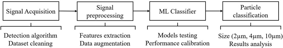
Figure 1. Overview of the ML pipeline developed for micro-particle size classification from SMI-sensor signals.

The paper is organized as follows: Section 2.1 explains the induced modulation due to single-particle transit. Section 2.2 describes the experimental setup for the SMI flow cytometer. Section 2.3 outlines the data acquisition and classification pipeline. Finally, Section 3 presents and discusses the classification results obtained from the different approaches.

2 Materials and methods

2.1 Theory

The self-mixing interferometry phenomenon arises from the interaction between the internal light wave propagating within the laser cavity and the portion of light backscattered by an external target that re-enters into the cavity, causing a modulation in the laser output power. In the context of this study, we focus exclusively on the single-particle case, where only one particle at a time crosses the laser beam, thus scattering light back into the laser cavity (Zhao et al., 2016). Under this condition, each photon is assumed to be scattered solely by that individual particle during its round-trip propagation. The case involving multiple scatterers has been addressed in various studies (Campagnolo, 2013; Atashkhooei et al., 2018). A general schematic of the effect involved is presented in Figure 2.

Figure 2

Figure 2. Schematic representation of an SMI sensor detecting the backscattered light from a single particle suspended in a fluid, moving at velocity V as it traverses the laser beam’s sensing volume.

Due to the Doppler effect, when a particle moves through the laser beam with a constant velocity $V$, the output power signal exhibits periodic modulation at the Doppler frequency shift $f_D$ (Albrecht et al., 2003). The value of $f_D$ depends on the incidence angle $\theta$ between the laser beam axis and the flow direction and the laser wavelength $\lambda$, as given by Equation 1:

$f_D=\frac{2V\sin \left(\theta \right)}{\lambda }(1)$

The initial modulation in the laser output power $P(t)$ due to the self-mixing effect is expressed in Equation 2, where $P_0$ represents the initial laser output power, $m$ is the modulation index, indicating the feedback strength, and ${\varphi }_D$ denotes the phase variation due to the Doppler frequency $f_D$, carrying information about the uniquely scattered particle.

$P\left(t\right)=P_0\left[1+m\cos \left(2\pi f_{D}t\right)\right](2)$

As a particle passes through the laser sensing volume, defined as the spatial region where sufficient light is scattered back from the particle to the laser and produces detectable modulation in the laser output power within our acquisition system, it experiences a Gaussian spatial intensity profile consistent with Gaussian beam theory. The modulation amplitude reaches its peak when the particle’s center crosses the central axis of the laser beam $k$ at $t=t_0$, gradually decreasing as the particle exits the interrogation zone (Zhao et al., 2023b). The final expression for the output power modulation resulting from particle transit is:

$P_F\left(t\right)=P_0\left[1+m\cos \left(2\pi f_{D}t\right)\right]e^{-\frac{{\left(t-t_0\right)}^2}{2{\tau }^2}}(3)$

Here, $\tau$ represents the particle’s transit time inside the laser beam, which can be estimated using the laser spot size $L_s$, the particle diameter $P_d$, and its velocity $V$ as presented in Equation 4:

$\tau =\frac{L_s+P_d}{V\sin \left(\theta \right)}(4)$

Figure 3A illustrates an example of the modulation induced in the laser output power by the passage of two 4 µm diameter spheres, each transiting through the laser sensing volume at different times. Figure 3B shows a filtered SMI signal corresponding to a single particle crossing the sensing volume, highlighting the Gaussian-shaped envelope that characterizes the amplitude burst. Finally, Figure 3C presents the characteristic Doppler frequency peak extracted from the filtered signal, which is directly related to the particle’s velocity.

Figure 3

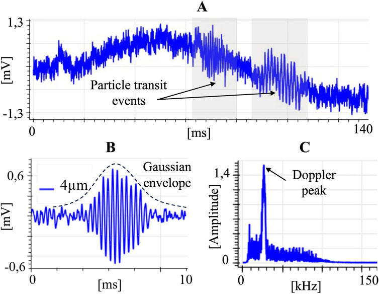
Figure 3. Experimental acquisition of the SMI signal during particle transit. (A) Raw SMI signal highlighting the passage of two particles at different times. (B) Filtered SMI signal corresponding to a 4 µm polystyrene sphere. (C) Frequency spectrum (FFT) of the filtered signal.

2.2 System overview

The schematic in Figure 4 illustrates the setup assembled for single-particle detection using the SMI sensing scheme. The system consists of two main subsystems: an optoelectronic system, responsible for enhancing and acquiring the SMI signal, and a microfluidic system, designed to control a consistent particle flow.

Figure 4

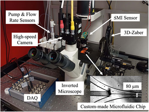
Figure 4. SMI flow cytometer experimental setup assembled, highlighting the main components of the system, including the microfluidic chip designed for single-particle isolation through the hydrodynamic focusing effect.

2.2.1 Optoelectronic subsystem

The optical setup employs a 1,550 nm single-mode distributed feedback (DFB) laser diode (ThorLabs-L1550P5DFB) equipped with a package-integrated monitoring photodiode. To ensure sufficient power and signal enhancement during particle passage, the laser beam is focused using a doublet lens (AC254-030-C), achieving a measured spot diameter of 80 μm at its waist with an initial power of 4.7 mW. The propagation axis of the laser is set at an angle of 80$°$ relative to the channel flow. The laser is mounted on a 3-axis linear stage (ZaberTech T-LSM050A) to allow precise micrometer-scale alignment. The SMI signal is acquired by monitoring variations in the photodiode current using a custom-made transimpedance amplifier and recorded at a sampling rate of 2 MHz using an acquisition card (DAQ NI-6361).

2.2.2 Microfluidic subsystem

To achieve single-particle alignment and ensure a constant flow of individual particles through the laser sensing volume, a custom-made PDMS microfluidic chip was fabricated, specifically designed to perform hydrodynamic focusing (HF) for particle alignment. The channel structure was created using photolithography, and its dimensions were verified using a profilometer, confirming a consistent height of 70 µm and a width of 80 µm. For particle isolation via HF, the flow rates are set at 5 μL/min for the sheath flow and 10 μL/min for the sample flow. The velocity profile inside the chip was estimated through simulations in COMSOL to determine the range of particle speeds within the chip. To verify the correct operation of the HF system, the microfluidic chip is mounted on an inverted microscope, allowing real-time monitoring of the channel and flow using a high-speed camera.

Inspired to simulate human blood cells for flow cytometry experiments, synthetic 2, 4, and 10 µm monodisperse polystyrene particles are used, each with a coefficient of variation of 1.8% in its diameter. For each particle size, a 4% concentration was prepared in 1 mL of deionized water (DI) and introduced into the channels using a microfluidic control system (Fluigent MFCS-EZ) equipped with multiple flow rate sensors (Fluigent Flow Unit M+) with a precision of $\pm$ 0.2 mL/min, allowing precise adjustment of the flow rate during experiments.

2.3 Pipeline

2.3.1 Signal acquisition

To construct a robust database containing the induced modulation caused by particle transit, all potential particle events were recorded in real-time using a Python-based acquisition routine. The collected signals were then analyzed to segment the time intervals corresponding to each particle’s passage for further analysis. Additionally, to increase the size of the dataset and improve model generalization, multiple augmentation techniques were applied.

The data acquisition system (DAQ) was configured with a sampling frequency of 2 MHz, chosen to cover the expected Doppler frequency peaks range while retaining higher-order harmonics and transient components, and to provide a comprehensive dataset for both algorithm development and later decimation analysis. Each acquisition window captured 8.192 ms (16,384 samples) to ensure full coverage of the slowest particle transits while limiting unrelated signal content. A real-valued FFT of the full segment with a rectangular window was applied to identify the characteristic Doppler peaks. This configuration balanced detection reliability, computational efficiency, and preservation of amplitude information in low-SNR conditions (Rapuano and Harris, 2008). To define a broad frequency range of interest, the expected particle velocity was estimated through numerical simulations. Based on Equation 1, a detection range from 5 kHz to 100 kHz was established, broad enough to avoid missing Doppler peaks outside the expected range while still allowing effective filtering of irrelevant frequencies. A threshold level for peak detection was determined experimentally by analyzing the noise level when only deionized (DI) water was flowing. Segments that met the detection criteria were stored for further processing.

2.3.2 Offline validation

Following the approach described in Sierra-Alarcón et al. (2024), an offline adaptive spectrogram algorithm was employed to extract only the signal segments corresponding to particle transits. For each detected event, the spectrogram parameters were adjusted based on the estimated particle velocity and transit duration. A Gaussian fit was then applied to verify whether the observed modulation matched the expected signal shape defined in Equation 3.

To support this validation, the signal-to-noise ratio (SNR) was evaluated using Equation 7, providing initial evidence that the signal amplitude decreases as particle size decreases (Figure 5). The SNR was estimated by comparing the average power of segments containing particle-induced modulation, $x_{\text{p}}(t)$, with those containing only noise signal, $x_{\text{np}}(t)$.

Figure 5

Figure 5. Representation of signal-to-noise ratio for different particle sizes. The red line represents the mean, the box indicates the standard deviation, and the blue lines show the maximum and minimum values.

The final dataset included 700 labeled samples for each particle size (2, 4, and 10 µm), with each sample spanning 1.25 ms (2,500 data points), capturing the complete transit event while excluding irrelevant portions of the signal.

$P_{\text{signal}}=\frac{1}{N}{\displaystyle \sum _{i=1}^N}{x}_{\text{p}}{\left(i\right)}^2(5)$

$P_{\text{noise}}=\frac{1}{N}{\displaystyle \sum _{i=1}^N}{x}_{\text{np}}{\left(i\right)}^2(6)$

$SNR\left(\mathrm{d}\mathrm{B}\right)=10\cdot {\log }_{10}\left(\frac{P_{\text{signal}}-P_{\text{noise}}}{P_{\text{noise}}}\right)(7)$

2.3.3 Data augmentation

A combination of the following data augmentation techniques was randomly applied to represent possible variation in the real raw signals while preserving the essential characteristics of the modulations.

$•$ Additive Noise: Gaussian noise is added to the signal to reduce the SNR in each sample. The noisy signal is given by Equation 8:

$x_{\text{noisy}}\left(t\right)=x\left(t\right)+\mathcal{N}\left(0,{\sigma }^2\right)(8)$

where $\mathcal{N}(0,{\sigma }^2)$ represents Gaussian noise with zero mean and variance ${\sigma }^2$.

$•$ Quantization: This technique reduces the resolution of the signal by constraining each sample to a fixed number of possible values. For a given resolution $R$, each sample $x(t)$ is transformed as Equation 9:

$x_{\text{qt}}\left(t\right)=\frac{\lfloor R\cdot x\left(t\right)\rfloor }{R}(9)$

where $\lfloor \cdot \rfloor$ represents the floor operation. Here, $R$ is a random integer selected between 40 and 100, for quantizing the signal and reducing its precision.

$•$ Downsampling: In this method, the temporal resolution of the signal is reduced by selecting a downsampling factor $k$ (randomly chosen between 2 and 9). For every $k$-th sample $x_i$, the next $k$ samples are overwritten with $x_i$, maintaining the original length of the signal. Mathematically, this can be as expressed in Equation 10:

$x_{\text{ds}}\left(i+j\right)=x\left(i\right),\forall j\in \left[0,k-1\right](10)$

$•$ Amplitude Inversion: The signal is inverted to simulate phase changes (Equation 11), achieved by multiplying the amplitude of the signal by $-1$:

$x_{\text{inverted}}\left(t\right)=-x\left(t\right)(11)$

$•$ Random Interpolation: A random subset of the signal is replaced by interpolated values to simulate missing or corrupted data following Equation 12. For a randomly chosen set of indices $\{i_1,i_2,\dots ,i_n\}$, the interpolated values are calculated as:

$x_{\text{it}}\left(i\right)=\text{inter}\left(i,\mathbf{x}\right)(12)$

where $\text{inter}$ denotes a linear interpolation function.

$•$ Shifting: To simulate variations in timing, the signal is circularly shifted by a factor $\mathrm{\Delta }t$, determined as a percentage of the signal length using Equation 13:

$x_{\text{shift}}\left(t\right)=x\left(\left(t+\mathrm{\Delta }t\right)\mathrm{mod}N\right)(13)$

where $N$ is the total number of data points.

2.4 Signal data preprocessing

To evaluate multiple approaches for the classification task and after the different augmentation techniques, three different data representations were explored: the use of the SMI temporal signal, an optimized spectrogram, and the classification based on specific features extracted from both the temporal and frequency spectrum of the signal, as illustrated in Figure 6.

Figure 6

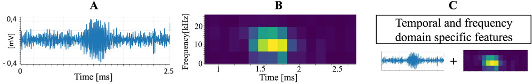
Figure 6. Data representations explored for the classification task. (A) Filtered SMI temporal signal modulation. (B) SMI signal spectrogram. (C) Handcrafted temporal and frequency features.

2.4.1 SMI temporal signal enhancement

To reduce signal dimensionality and suppress embedded noise, all samples were processed using a band-pass filter based on the previously defined frequency ranges. A decimation step was then applied, reducing the sampling rate by a factor of 4, to 500 kHz. This reduction aimed to decrease data size without significantly altering the signal characteristics. Additionally, the filtered signals were scaled by a factor of 10, selected after testing different values (1, 5, 10, 20) for its ability to accelerate convergence by increasing gradient magnitudes, without affecting classification accuracy or altering the relative shape of the signals (LeCun et al., 2012). This formatted signal was then used for the next data representation approaches.

2.4.2 Spectrogram-based features

Time-domain spectral analysis is essential for capturing the dynamic behavior of non-stationary signals by revealing how their frequency content evolves over time. Spectrograms were employed due to their effectiveness in detecting transient events and frequency variations. The spectrogram is computed using the Short-Time Fourier Transform (STFT), as defined in Equation 14

$S\left(t,f\right)={\int }_{-\infty }^{\infty }x\left(\tau \right)w\left(\tau -t\right)e^{-j2\pi f\tau }d\tau (14)$

where $x(\tau )$ represents the signal, $w(\tau -t)$ is the Hamming window centered at time $t$, and $f$ is the frequency. The computation of $S(f,t)$ involves three key parameters: $N_{\text{perseg}}$, which defines the length of the window function $w[n-\tau ]$; $N_{\text{overlap}}$, which specifies the overlap between consecutive windows (typically set to half of $N_{\text{perseg}}$ to ensure effective detection of transient events); and $F_{\text{range}}$, which determines the frequency range under consideration. The selection of spectrogram parameters was guided by the Doppler frequency range of detected peaks in real particle samples, refining the analysis to focus specifically on the Doppler frequency component and its decay over time (5–40 kHz). This was done while considering the passage duration of the smallest, fastest particles in the dataset. The frequency resolution is given by Equation 15:

$\mathrm{\Delta }f=\frac{f_s}{N_{\text{perseg}}}(15)$

where $f_s=500\text{\hspace{0.17em}kHz}$ is the sampling rate. To achieve a target frequency resolution of 1 kHz, the required window length is $N_{\text{perseg}}=500$ samples. This corresponds to a temporal resolution of approximately 1 ms.

This configuration ensures that short-duration events, such as those caused by 2 $\mu$m particles lasting approximately 1.6 ms, remain visible while preserving spectral integrity.

The choice of spectrograms over alternative representations, such as Mel-Frequency Cepstral Coefficients (MFCCs), was based on their ability to preserve raw time-frequency relationships (Zhao K. et al., 2020; Gourisaria et al., 2024). While MFCCs are effective for auditory perception tasks, they involve dimensionality reduction and feature decorrelation, which can lead to information loss and increased noise sensitivity in non-speech signals. In contrast, spectrograms provide a richer representation, facilitating the extraction of meaningful patterns while maintaining correlated spectral features.

2.4.3 Specific features

To extract valuable information from both the temporal and frequency domains and to improve differentiation where particle modulation is embedded in noise, the following features were defined:

$•$ Signal Amplitude: The amplitude of the temporal signal correlates with particle size, as larger particles induce higher voltage variations. To ensure robustness against noise-induced peaks, the amplitude is extracted using the envelope of the absolute signal. The envelope is computed using the Hilbert transform (Zhao et al., 2019), providing a smooth upper bound that mitigates the impact of noise peaks.

$•$ Passage Time: quantifies the duration for which a particle remains within the laser beam’s sensing volume. This feature is extracted by analyzing the parabolic modulation of the signal, modeled using a Gaussian fit applied to the envelope (Sierra-Alarcón et al., 2024). The passage interval is defined as the period during which the Gaussian fit remains above 10% of its peak amplitude, accounting for the SNR in smaller particles such as those with a 2 µm diameter.

$•$ Average Signal Power: Reflecting the overall signal intensity, this feature may correlate with particle size since larger particles induce stronger modulations (Equation 16). It is computed following the same approach as the SNR:

$S_{\text{avg}}=\frac{1}{N}{\displaystyle \sum _{i=1}^N}{x}_{\text{p}}{\left(i\right)}^2-\frac{1}{N}{\displaystyle \sum _{i=1}^N}{x}_{\text{np}}{\left(i\right)}^2(16)$

where $N$ is the total of data points in a sample.

$•$ Frequency Spectrum Power: This feature quantifies the total signal energy distributed over the time-frequency domain, estimated from the STFT. It reflects the overall energy content of the signal across all time and frequency bins according to Equation 17.

$F_{\text{spec}}={\displaystyle \sum _t}{\displaystyle \sum _f}|STFT\left(t,f\right){|}^2(17)$

$•$ Peak Spectral Amplitude: This feature captures the highest spectral amplitude observed in the STFT magnitude, corresponding to the strongest frequency component. It provides insight into the most dominant spectral peak and can be useful for identifying particles that produce sharp localized energy bursts following Equation 18.

$F_{\text{peak}}=\underset{t,f}{\max }\left\{|STFT\left(t,f\right)|\right\}(18)$

$•$ Doppler Frequency: Extracted by identifying the highest peak in the frequency spectrum after applying the Fourier Transform (Equation 19).

$f_{\text{Doppler}}=\arg \underset{f}{\max }\left\{X\left(f\right)\right\}(19)$

2.4.4 T-SNE analysis for feature space visualization

To qualitatively assess the discriminative capacity of the extracted features, a t-SNE (t-distributed Stochastic Neighbor Embedding) projection was applied to both the handcrafted and spectrogram-based feature sets. This dimensionality reduction technique maps high-dimensional data into a two-dimensional space while preserving local structure, allowing for visual inspection of class separability and the clustering behavior of the features (Maaten and Hinton, 2008). Figure 7 presents the resulting t-SNE plots, where each point corresponds to a sample, and colors indicate particle size classes. The resulting spatial distribution suggests that the extracted features contain sufficient information to support particle size classification.

Figure 7

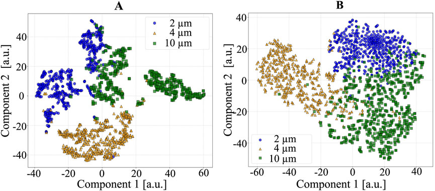
Figure 7. T-SNE visualization of feature representations for the three different particle sizes. (A) Handcrafted features. (B) Spectrogram-based features.

2.5 ML classifier models

Machine learning models, specifically deep learning architectures, were evaluated using different input representations, with hyperparameters optimized via grid search based on their impact on model performance (Yang and Shami, 2020). The dataset was randomly shuffled prior to data augmentation, with 30% allocated for testing using real particle signals and the remaining 70% used for training and validation. This training portion was subsequently augmented and split into 80% for training and 20% for validation. Model performance was evaluated in terms of classification accuracy and computational efficiency, as detailed in the Appendix.

2.5.1 Spectrogram-based model

This model processes spectrograms resized to dimensions $63\times 65\times 1$, which are then passed through a fully connected neural network. The architecture includes a Flatten layer, followed by two dense layers, each using ReLU activation, batch normalization, and L2 regularization with a coefficient $\lambda =2.5\times 10^{-4}$ to improve generalization (Yang and Shami, 2020; Agrawal, 2021). Dropout is applied after each dense layer to prevent overfitting. The output layer consists of three neurons with softmax activation, corresponding to the three particle size classes. Training was conducted using a batch size of 32 and the Adam optimizer with a learning rate decay initialized at $6\times 10^{-4}$, using categorical cross-entropy as the loss function. Early stopping was implemented to further reduce overfitting by monitoring validation loss.

All model hyperparameters were optimized via grid search. This included the STFT parameter $\text{nperseg}=2^n$, with $n\in [\mathrm{7,9}]$, dropout rates $p_{\text{dropout}}\in [0.1,0.2]$, and dense layer sizes dense1, dense2 $=2^n$, with $n\in [\mathrm{3,8}]$. The optimal configuration, which also reflects the most effective spectrogram resolution, was found to be dense1 = 64, dense2 = 8, $p_{\text{dropout}}=0.1$, and $\text{nperseg}=128$. This configuration achieved a test accuracy of 97.7% and a validation accuracy of 98.6%.

2.5.2 Feature-based model

Following a similar topology to the spectrogram-based model, this version replaces the spectrogram inputs with engineered statistical and frequency-domain features, which are normalized using Z-score scaling. The training methodology remains unchanged, with the L2 regularization coefficient adjusted to $\lambda =1\times 10^{-4}$. Hyperparameter tuning explored dense layer sizes defined as $\text{dense}1,\text{dense}2=2^n$, with $n\in [\mathrm{5,6,7,8,9}]$, and dropout rates $p_{\text{dropout}}\in [0.1,0.2]$.

The best configuration was achieved with $\text{dense}1=128$, $\text{dense}2=256$, and $p_{\text{dropout}}=0.1$. This feature-based model achieved a test accuracy of 97.0% and a validation accuracy of 97.8%.

2.5.3 SMI temporal signal-based model

The 1D Convolutional Neural Network (CNN) model was developed for temporal signal classification, following the band-pass filtering and decimation steps and employing a hierarchical feature extraction strategy. The architecture is composed of three convolutional layers with an increasing number of filters $2^n$ with $n\in [6-8]$ and a kernel size of 5. Each layer uses ReLU activation to capture temporal patterns within the waveform. Batch normalization is applied after each convolutional layer to stabilize the training process, followed by MaxPooling1D (pool size = 2) to reduce dimensionality while preserving relevant temporal features. To prevent overfitting, a dropout rate of $p_{\text{dropout}}=0.2$ is applied after each pooling layer.

The extracted features were then flattened and passed through a fully connected dense layer with 256 neurons and L2 regularization $(\lambda =1\times 10^{-4})$, before reaching the softmax output layer with three neurons corresponding to the particle size classes. The model is trained using the Adam optimizer with a learning rate of $6\times 10^{-4}$, employing categorical cross-entropy loss. All hyperparameters were tuned via grid search. This CNN model achieved a test accuracy of 98.9% and a validation accuracy of 98.3%.

3 Results and discussion

Figure 8 presents the classification performance achieved across the different ML models, showing a high level of accuracy in correctly predicting each particle category. To complement the accuracy results and provide a more complete evaluation, Table 1 details the precision (P), recall (R), and F1-score (F1) for each particle size and model.

Figure 8

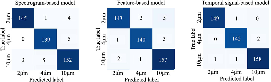
Figure 8. Confusion matrix showing the classification performance across different ML models: the spectrogram-based model, the feature-engineered model, and the SMI temporal signal-based model.

Table 1

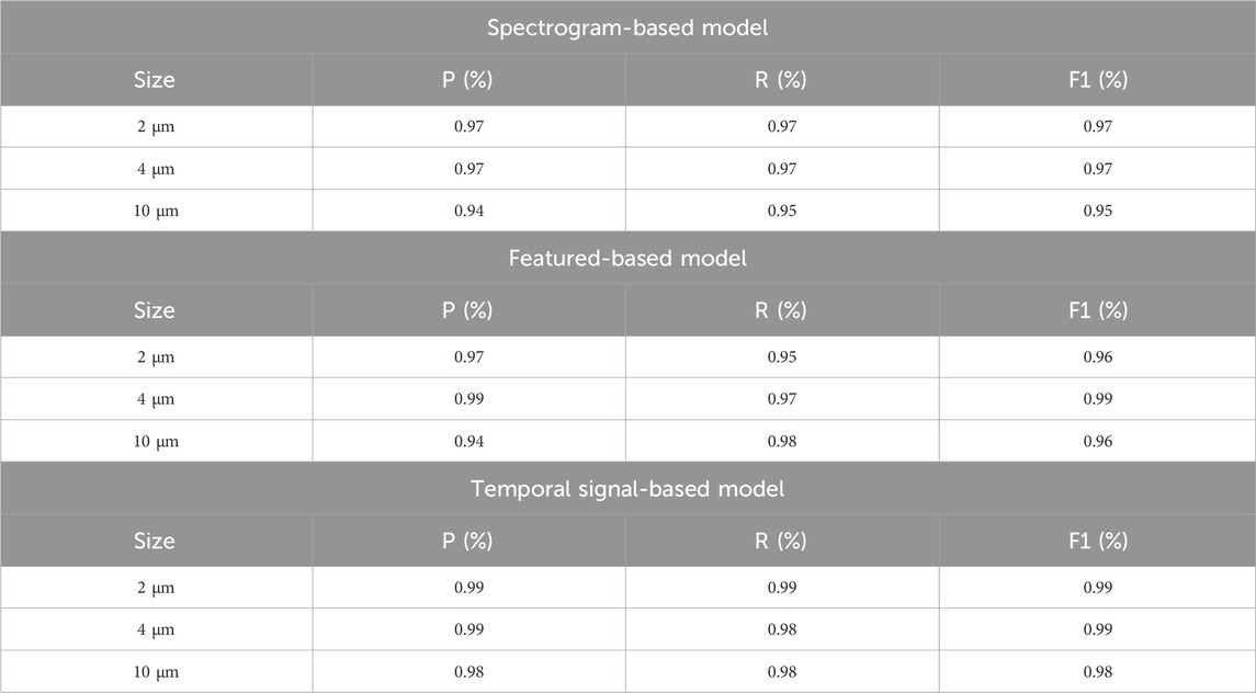
Table 1. Detailed classification results for each particle type based on different data representations, including the model’s precision (P%), recall (R%), and F1-score (F1%).

The results confirm that the proposed signal analysis pipeline enables a reliable and consistent particle classification system, as all data representations achieved accuracy values close to 98% and maintained precision, recall, and F1-scores above 94% across all classes. The temporal signal-based model achieved the most balanced performance, with all three metrics in the 0.98–0.99 range, indicating consistent detection with minimal false positives and false negatives. The spectrogram-based and feature-engineered models also yielded strong results, although slightly lower recall for 2 µm particles (0.95) suggest occasional misclassification for the smaller particles sizes.

These findings align with the dimensionality reduction analysis, where particle sizes were well separated in the 2D feature space, indicating that the classification task is not overly complex. Additionally, the relatively simple architectures used in the spectrogram-based and feature-engineered models, consisting of only two dense layers, reinforce that the chosen data representations provided sufficient discriminative information for accurate classification. Even for the most challenging case (2 µm particles), the system maintained a 97% of accuracy, indicating strong classification performance.

On the other hand, the temporal SMI signal-based model demonstrated effective classification without significantly increasing model complexity. Despite having only three convolutional layers and a single dense layer, this model achieved comparable performance, demonstrating that even a small deep learning model can successfully classify particles. This is particularly relevant for real-time implementation, as the raw signal model eliminates the need for explicit feature extraction steps, showcasing the powerful feature learning and generalization capabilities of SMI signals.

To further analyze the computational performance of the models, quantization techniques were applied by reducing data precision from floating-point (FP64) to integer 8-bit (Int8). The results indicate that classification accuracy remained unaffected, confirming that the quantization process did not degrade model performance, likely due to the model’s small size, allowing quantization to reduce storage size, RAM usage, and inference latency without significant loss of accuracy.

Table 2 presents the storage, inference latency, and peak RAM usage of each model before and after quantization. Notably, the raw signal model, despite handling unprocessed data, required only 2.16 MB of storage and achieved a theoretical inference time of 1.8 ms. The spectrogram-based and feature-engineered models exhibited lower storage and RAM consumption but with slightly higher inference latency. These computational metrics were validated using TensorFlow Lite profiling, confirming that the models are suitable for deployment on low-power and resource-constrained devices. However, further evaluation on embedded hardware remains necessary to validate real-world performance. These findings demonstrate that high-performance classification is achievable without requiring large-scale models.

Table 2

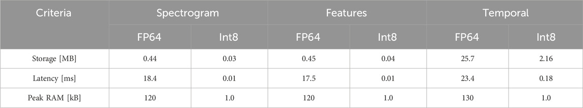
Table 2. Computational efficiency metrics for different data representations and precisions across ML models, including storage size, inference latency, and RAM usage.

The present evaluation employed monodisperse polystyrene particles, providing a controlled and repeatable test case for assessing the system’s baseline performance. Future work will focus on extending the analysis to heterogeneous mixtures containing particles of different sizes, shapes, and materials, including biological cells. This will allow for a more comprehensive assessment of the model’s robustness in complex, application-relevant scenarios, while expanding the dataset of SMI signals and validating performance under conditions representative of practical flow cytometry tasks.

Additionally, enhancements in both the optical and microfluidic components of the system are anticipated. Optimizing the received laser feedback, exploring alternative light sources such as VCSELs with more uniform light distribution, and refining hydrodynamic focusing, potentially by incorporating 3D hydrodynamic effects to ensure more consistent particle alignment and velocity, will be key to further improving the system’s performance.

4 Conclusion

This study proposed a machine learning pipeline for classifying particles in self-mixing interferometry signals, enhancing the accuracy of real-time particle analysis. The approach integrated data acquisition, filtering, data augmentation, and three data representations: spectrogram-based, feature-engineered, and temporal signal-based models. The results demonstrated that both fully connected neural networks and 1D convolutional networks achieved high classification accuracy, reaching up to 98% for particle size classification. These findings validate the effectiveness of the proposed pipeline in distinguishing particle sizes across varying signal-to-noise ratios. Moreover, the model architectures were computationally efficient, with low inference times, making them suitable for deployment on low-power embedded systems. This research highlights the potential of machine learning in improving the robustness and reliability of SMI-based particle classification and contributes to the advancement of real-time, label-free SMI particle analysis, with direct applications in medical sensing and flow cytometry. Future work will focus on handling more complex particle mixtures, integrating models into embedded systems such as microcontrollers or FPGAs, and further optimizing real-time classification applications.

Data availability statement

The raw data supporting the conclusions of this article will be made available by the authors, without undue reservation.

Author contributions

SS: Conceptualization, Data curation, Formal Analysis, Investigation, Methodology, Validation, Visualization, Writing – original draft, Writing – review and editing. JP: Conceptualization, Formal Analysis, Funding acquisition, Investigation, Resources, Supervision, Writing – original draft, Writing – review and editing. CT: Conceptualization, Resources, Writing – review and editing. FJ: Conceptualization, Resources, Writing – review and editing. AQ: Conceptualization, Formal Analysis, Funding acquisition, Investigation, Project administration, Resources, Supervision, Validation, Writing – review and editing.

Funding

The author(s) declare that financial support was received for the research and/or publication of this article. The author(s) declare that this work received financial support from the LAAS-CNRS Micro and Nanotechnologies Platform, a member of the French Renatech network, for the research and/or publication of this article.

Conflict of interest

The authors declare that the research was conducted in the absence of any commercial or financial relationships that could be construed as a potential conflict of interest.

Generative AI statement

The author(s) declare that no Generative AI was used in the creation of this manuscript.

Any alternative text (alt text) provided alongside figures in this article has been generated by Frontiers with the support of artificial intelligence and reasonable efforts have been made to ensure accuracy, including review by the authors wherever possible. If you identify any issues, please contact us.

Publisher’s note

All claims expressed in this article are solely those of the authors and do not necessarily represent those of their affiliated organizations, or those of the publisher, the editors and the reviewers. Any product that may be evaluated in this article, or claim that may be made by its manufacturer, is not guaranteed or endorsed by the publisher.

References

Agrawal, T. (2021). Hyperparameter optimization in machine learning: make your machine learning and deep learning models more efficient. Springer.

Google Scholar

Albrecht, H.-E., Borys, M., Damaschke, N., and Tropea, C. (2003). Laser Doppler and phase Doppler measurement techniques. Springer, 9–26. doi:10.1007/978-3-662-05165-8_2

CrossRef Full Text | Google Scholar

An, L., and Liu, B. (2022). Measuring parameters of laser self-mixing interferometry sensor based on back propagation neural network. Opt. Express 30, 19134–19144. doi:10.1364/OE.460625

PubMed Abstract | CrossRef Full Text | Google Scholar

Atashkhooei, R., Ramírez-Miquet, E. E., Moreira, R. d. C., Quotb, A., Royo, S., and Perchoux, J. (2018). Optical feedback flowmetry: impact of particle concentration on the signal processing method. IEEE Sensors J. 18, 1457–1463. doi:10.1109/JSEN.2017.2781902

CrossRef Full Text | Google Scholar

Barland, S., and Gustave, F. (2021). Convolutional neural network for self-mixing interferometric displacement sensing. Opt. Express 29, 11433–11444. doi:10.1364/OE.419844

PubMed Abstract | CrossRef Full Text | Google Scholar

Campagnolo, L., Nikolić, M., Perchoux, J., Lim, Y. L., Bertling, K., Loubiere, K., et al. (2013). Flow profile measurement in microchannel using the optical feedback interferometry sensing technique. Microfluid. Nanofluid. 14, 113–119.

CrossRef Full Text | Google Scholar

Chen, J., Wang, X., He, C., and Wang, M. (2024). Optical shaping self-mixing interferometry with a neural network for displacement measurement. J. Opt. Soc. Am. B 41, 1947–1952. doi:10.1364/JOSAB.533685

CrossRef Full Text | Google Scholar

Da Costa Moreira, R., Perchoux, J., Zhao, Y., Tronche, C., Jayat, F., and Bosch, T. (2017). “Single nano-particle flow detection and velocimetry using optical feedback interferometry,” in 2017 IEEE Sensors, Glasgow, UK, 29 October 2017 - 01 November 2017 (IEEE). doi:10.1109/icsens.2017.8234105

CrossRef Full Text | Google Scholar

Donati, S., and Norgia, M. (2014). Self-mixing interferometry for biomedical signals sensing. IEEE J. Sel. Top. Quantum Electron. 20, 104–111. doi:10.1109/JSTQE.2013.2270279

CrossRef Full Text | Google Scholar

Gourisaria, M., Agrawal, R., Sahni, M., and Singh, P. (2024). Comparative analysis of audio classification with mfcc and stft features using machine learning techniques. Discov. Internet Things 4, 1. doi:10.1007/s43926-023-00049-y

CrossRef Full Text | Google Scholar

Ha, M.-K., Phan, T.-L., Nguyen, D. H. H., Quan, N. H., Ha-Phan, N.-Q., Ching, C. T. S., et al. (2023). Comparative analysis of audio processing techniques on doppler radar signature of human walking motion using cnn models. Sensors 23, 8743. doi:10.3390/s23218743

PubMed Abstract | CrossRef Full Text | Google Scholar

Herbert, J., Bertling, K., Taimre, T., Rakić, A., and Wilson, S. (2018). Microparticle discrimination using laser feedback interferometry. Opt. Express 26, 25778. doi:10.1364/oe.26.025778

PubMed Abstract | CrossRef Full Text | Google Scholar

LeCun, Y. A., Bottou, L., Orr, G. B., and Müller, K.-R. (2012). Efficient BackProp. Berlin, Heidelberg: Springer Berlin Heidelberg, 9–48. doi:10.1007/978-3-642-35289-8_3

CrossRef Full Text | Google Scholar

Maaten, V. D. L., and Hinton, G. (2008). Visualizing Data using t-SNE. J. Mach. Learn. Res. 9, 2579–2605. Available online at: http://jmlr.org/papers/v9/vandermaaten08a.html

Google Scholar

Novac, P.-E., Rodriguez, L., and Barland, S. (2024). “Integrating embedded neural networks and self-mixing interferometry for smart sensors design,” in 2024 IEEE Sensors Applications Symposium (SAS), Naples, Italy, 23-25 July 2024 (IEEE).

CrossRef Full Text | Google Scholar

Perchoux, J., Quotb, A., Atashkhooei, R., Azcona, F., Ramírez-Miquet, E., Bernal, O., et al. (2016). Current developments on optical feedback interferometry as an all-optical sensor for biomedical applications. Sensors 16, 694. doi:10.3390/s16050694

PubMed Abstract | CrossRef Full Text | Google Scholar

Quotb, A., Atashkhooei, R., Magaletti, S., Jayat, F., Tronche, C., Goechnahts, J., et al. (2021). Methods and limits for micro scale blood vessel flow imaging in scattering media by optical feedback interferometry: application to human skin. Sensors 21, 1300. doi:10.3390/s21041300

PubMed Abstract | CrossRef Full Text | Google Scholar

Rapuano, S., and Harris, F. J. (2008). An introduction to fft and time domain windows. IEEE Instrum. Meas. Mag. 10, 32–44. doi:10.1109/mim.2007.4428580

CrossRef Full Text | Google Scholar

Sierra-Alarcón, S., Perchoux, J., Jayat, F., Tronche, C., Pérez, S. S., and Quotb, A. (2024). “Adaptive single micro-particle detection and segmentation in self-mixing interferometry signals,” in 2025 IEEE Applied Sensing Conference (APSCON) (IEEE).

Google Scholar

Taimre, T., Nikolić, M., Bertling, K., Lim, Y., Bosch, T., and Rakić, A. (2015). Laser feedback interferometry: a tutorial on the self-mixing effect for coherent sensing. Adv. Opt. Photonics 7, 570. doi:10.1364/aop.7.000570

CrossRef Full Text | Google Scholar

Yang, L., and Shami, A. (2020). On hyperparameter optimization of machine learning algorithms: theory and practice. Neurocomputing 415, 295–316. doi:10.1016/j.neucom.2020.07.061

CrossRef Full Text | Google Scholar

Zhao, Y., Perchoux, J., Campagnolo, L., Camps, T., Atashkhooei, R., and Bardinal, V. (2016). Optical feedback interferometry for microscale-flow sensing study: numerical simulation and experimental validation. Opt. Express 24, 23849–23862. doi:10.1364/OE.24.023849

PubMed Abstract | CrossRef Full Text | Google Scholar

Zhao, Y., Zhang, M., Zhang, C., Yang, W., Chen, T., Perchoux, J., et al. (2019). Micro particle sizing using hilbert transform time domain signal analysis method in self-mixing interferometry. Appl. Sci. 9, 5563. doi:10.3390/app9245563

CrossRef Full Text | Google Scholar

Zhao, K., Jiang, H., Wang, Z., Chen, P., Zhu, B., and Duan, X. (2020a). Long-term bowel sound monitoring and segmentation by wearable devices and convolutional neural networks. IEEE Trans. Biomed. Circuits Syst. 14, 985–996. doi:10.1109/TBCAS.2020.3018711

PubMed Abstract | CrossRef Full Text | Google Scholar

Zhao, Y., Shen, X., Zhang, M., Yu, J., Li, J., Wang, X., et al. (2020b). Self-mixing interferometry-based micro flow cytometry system for label-free cells classification. Appl. Sci. 10, 478. doi:10.3390/app10020478

CrossRef Full Text | Google Scholar

Zhao, Y., Li, J., Zhang, M., Chen, T., and Zou, J. (2023a). Investigation of the multiple characteristics of the self-mixing effect subject to a single particle. Opt. Express 31, 5458. doi:10.1364/oe.478821

PubMed Abstract | CrossRef Full Text | Google Scholar

Zhao, Y., Li, J., Zhang, M., Zhao, Y., Zou, J., and Chen, T. (2023b). Phase-unwrapping algorithm combined with wavelet transform and hilbert transform in self-mixing interference for individual microscale particle detection. Chin. Opt. Lett. 21, 041204. doi:10.3788/col202321.041204

CrossRef Full Text | Google Scholar

Appendix: classification metrics

Classification Accuracy Metrics

$•$ Accuracy: The proportion of correctly classified instances relative to the total number of samples.

$•$ Confusion Matrix: A detailed comparison of predicted classifications versus actual labels, highlighting classifications and misclassifications.

$•$ Precision (P): The fraction of correctly classified particles out of all predicted positive instances, minimizing false positives.

$•$ Recall (R): The model’s ability to identify all actual particle instances, reducing false negatives.

$•$ F1-score (F1): The harmonic mean of precision and recall, providing a balanced evaluation of classification performance.

Computational Efficiency Metrics

$•$ Storage Size: The total memory required to store the trained model, impacting its deployment on embedded platforms.

$•$ Inference Latency: The theoretical time required for the model to make a prediction, determining its suitability for real-time applications.

$•$ RAM Consumption: The peak dynamic memory usage during inference, critical deployment on low-memory devices.