Invisible footprints, visible insights: machine learning reveals Scope 3 emissions

Introduction: Scope 3 greenhouse gas emissions are critical to firms’ carbon footprints yet are often difficult to quantify due to limited direct data, motivating predictive modeling approaches.

Methods: We developed and compared four machine learning algorithms (K-nearest neighbors, random forest, AdaBoost, and XGBoost) to estimate corporate Scope 3 emissions using readily available financial and sustainability performance data. We leverage 10,449 listed firm-level data from 2014 to 2023, covering major industries such as semiconductor, steel, textile, and building materials, evaluating performance of each model by a held-out test set with metrics including R², mean absolute percentage error (MAPE), and root mean squared logarithmic error (RMSLE).

Results: XGBoost achieved the highest accuracy (R² = 0.85, MAPE = 15%, RMSLE = 0.20), outperforming random forest (R² = 0.80, MAPE = 20%) and AdaBoost (R² = 0.78), while K-NN had the lowest accuracy (R² = 0.60). The results demonstrate that ensemble tree-based models substantially improve Scope 3 emission prediction accuracy over simpler models.

Discussion: Notably, random forest’s interpretable feature importance provided insight into key emission drivers with only a slight accuracy trade-off, highlighting the balance between predictive accuracy and model interpretability.

1 Introduction

For most companies, the management of Scope 3 carbon emissions is a daunting and critical challenge. Such emissions cover carbon emissions from all indirect sources throughout the company’s entire value chain, including the activities of upstream suppliers and the downstream product use stage, and often constitute a major part of the company’s total carbon footprint (Khurana et al., 2021; Schmidt et al., 2022). Compared with Scope 1 and Scope 2 emissions, which are usually directly related to the company’s own operations and are easier to monitor and control, Scope 3 emissions occur outside the company’s operational boundaries, and its management relies on data support from multiple stakeholders such as suppliers, service providers and end users. The diversity of data sources, inconsistent reporting standards and highly decentralized supply chain structures all lead to difficulties and uncertainties in collecting emissions information. In the absence of transparent and consistent value chain emissions data, companies find it difficult to accurately grasp their own emission reduction progress, and are unable to effectively identify activities with higher emission intensity in operations and supply chains, which in turn limits their ability to formulate and implement carbon reduction measures that are consistent with ESG strategic goals (Busch et al., 2022).

Machine Learning (ML) has shown potential in improving the accuracy and reliability of carbon emissions (Tang et al., 2023; Zhang et al., 2022a, 2022b; Magazzino and Mele, 2022). Compared to traditional statistics, machine learning models have shown greater predictive power and adaptability in predicting CO2 and other pollutant emissions (Bai, 2023; Jain et al., 2023). Some academics have also extended the application of machine learning techniques to the estimation of Scope 3 emissions by analyzing corporate financial data and transaction records to model indirect carbon emissions in the value chain (Serafeim and Velez Caicedo, 2022; Jain et al., 2023). These results demonstrate the advantages of machine learning in dealing with complex structural data and incomplete information, and provide companies and policy makers with more actionable carbon management tools.

However, there are still significant gaps in the existing literature in several important aspects. Most studies are limited to specific industry sectors or only use a narrow combination of input variables, such as basic financial indicators, and have not fully incorporated more representative data such as operational aspects or industry characteristics. More importantly, there are currently few studies that systematically compare multiple machine learning algorithms under a consistent methodological framework to evaluate their trade-offs between predictive performance and practical usability, especially in the application scenario of Category III carbon emission estimation. This research gap is particularly critical because Category III emissions usually account for the largest proportion of a company’s total GHG emissions, even far higher than the sum of Category I and Category II (Huang et al., 2021; Khan and Kahn, 2020). If emissions in Category 3 are ignored, the actual carbon footprint of the company may be significantly underestimated, which may also mislead stakeholders and undermine the formulation of effective carbon reduction strategies (Schmidt et al., 2022; Wiedmann and Minx, 2008).

This study contributes to the literature on Scope 3 emission estimation in the following three aspects: First, this study builds a machine learning framework to systematically compare the prediction performance of several commonly used algorithms, including K-nearest neighbor, Random Forest, AdaBoost, and XGBoost, and overcomes the limitations of inconsistency and inaccuracy of the data that are common to the traditional estimation methods. Second, the proposed model integrates firm-level financial statement variables, Scope 1 and Scope 2 emission data, and industry classification information, providing a cost-effective and scalable tool for carbon emission estimation, which is particularly suitable for firms that lack detailed supply chain information. Third, this study further evaluates the trade-off between model predictive accuracy and interpretability, and discusses its implications for practical sustainability management, so as to assist sustainability managers in their quest for credible predictions while at the same time gaining insights that are valuable for decision-making.

The remainder of this paper is organized as follows. Section 2 presents a review of the pertinent literature on Scope 3 emissions estimation and machine learning applications. Section 3 introduces the dataset and methodological framework. Section 4 discusses the empirical results, including performance comparisons and model interpretability analysis. Section 5 concludes with practical implications and suggestions for future research.

2 Literature review and hypothesis development

2.1 Scope 3 emission

Carbon emissions research initially focused on Scope 1 and Scope 2 emissions, mainly because these two sources of emissions are relatively easy to quantify. Scope 1 covers direct emissions from a firm’s own operations, while Scope 2 includes indirect energy emissions such as purchased electricity, heat and steam (Wiedmann and Minx, 2008). In the early days, tracking these two domains was limited because firms could accurately calculate emissions through direct operational data (Valls-Val and Bovea, 2021). Over time, indirect emissions occurring up and down the corporate value chain (i.e., Scope 3) tend to be much higher than the sum of Scopes 1 and 2, prompting a shift in focus towards a more comprehensive carbon accounting framework (Khurana et al., 2021; Serafeim and Velez Caicedo, 2022). Several studies have now pointed out that Scope 3 emissions often constitute the largest part of a company’s overall carbon footprint, and that neglecting this part of a company’s carbon footprint may seriously underestimate its actual environmental impact (Wiedmann and Minx, 2008; Schmidt et al., 2022).

In parallel, motivated by policy developments such as Kyoto Protocol and Carbon Border Adjustment Mechanism, extensive literature has emerged focusing on carbon pricing mechanisms as a method to mitigate carbon emission (Nelson et al., 2012; Chevallier, 2013). Unlike the direct measurement of carbon emissions, the literature on carbon pricing models can generally be categorized into four main types: structural models, econometric models, stochastic models, and game-theoretic models (Chevallier, 2013; Nelson et al., 2012). These frameworks offer holistic syntheses of their theoretical foundations and empirical effectiveness (Jha et al., 2025; Çanakoğlu et al., 2018). Additional research provide in-depth analyses or forecasts of carbon pricing based on external market indicators, such as energy prices and financial indices (Carraro and Favero, 2009; Christiansen et al., 2005; Guðbrandsdóttir and Haraldsson, 2011; Aatola et al., 2013; Yahşi et al., 2019).

The estimation of carbon emissions in Scope 3 is methodologically more complex than the more straightforward calculation of Scope 1 and Scope 2. Scope 3 covers indirect emissions generated in the upstream and downstream value chains of firms, which are not under the direct control of the firms themselves, making it challenging to obtain and calculate information (Huang et al., 2021; Khan and Kahn, 2020). In view of this, in recent years, scholars have begun to look for alternative sources of data, such as financial statements, procurement records, and industry-level statistics, which can be combined with operational information already used by firms to estimate Scope 1 and Scope 2 to help improve the accuracy of Scope 3 emissions estimates (Serafeim and Velez Caicedo, 2022; Nguyen et al., 2023). In response to this estimation challenge of high data fragmentation and information gaps, researchers have gradually introduced advanced analytical tools, including machine learning techniques, which can integrate heterogeneous data sources and effectively model and interpret them, and have been regarded as an important method to improve the performance of Scope 3 emission estimation (Tang et al., 2023; Zhang et al., 2022a, 2022b).

2.2 Leveraging machine learning to estimate Scope 3

Scope 3 has been the focus of attention in previous emission projection studies. While there are a variety of methods for analyzing Scope 3 emissions, the dominant approach is to use machine learning for the analysis. Collecting Scope 3 data through traditional statistical methods is likely to yield reliable results due to the completeness of the data and consistent reporting. The advantage of using machine learning is that it increases accuracy and significantly improves the estimation of upstream carbon emissions. In addition, it excels in data processing and trend analysis (Nguyen et al., 2021; Wang et al., 2024).

Khan and Kahn (2020) show that machine learning algorithms are able to process large and complex datasets to capture potential non-linear relationships among variables, which in turn improves the accuracy of carbon emission estimation. Similarly, Hsu and Kwan (2020) explored the potential application of deep learning models for greenhouse gas (GHG) emission prediction, especially in handling indirect emission estimation associated with the domain three reporting framework, which demonstrated higher accuracy and prediction capability.

Previous studies using machine learning to predict corporate Scope 3 carbon emissions have included predictions based on companies in different countries or regions (Javanmard and Ghaderi, 2022; Magazzino and Mele, 2022; Bhatt et al., 2023; Natarajan et al., 2024). The policies of these countries or regions often vary due to historical factors, making it necessary to predict the behavior of companies with different approaches. As sustainability becomes increasingly important (de Oliveira et al., 2024), the business world can observe carbon emission outcomes and differences across countries or regions.

Scope 3 Machine learning (ML) analysis has been shown to outperform traditional statistical methods. For example, Zhang et al. (2022a, 2022b) report that ML models outperform traditional statistical analysis in predicting fine particulate matter (PM) concentrations. Similarly, Magazzino and Mele (2022) observed that ML methods can mitigate problems such as omitted variable bias and endogeneity relative to ordinary least squares (OLS) regression. These advantages are due in part to the fact that ML techniques provide greater flexibility in the specification of the functional form and allow for more efficient selection of features to avoid overfitting (Zhang et al., 2022a, 2022b). In the context of Scope 3 emissions, researchers have begun to integrate variables other than basic financial metrics to improve prediction accuracy. For example, Serafeim and Velez Caicedo (2022) developed ML models for multiple Scope 3 categories with input features from company financial statements. Their approach includes balance sheet “stock” metrics (e.g., total assets), income statement “flow” metrics (e.g., revenue), and financial ratios (e.g., capital intensity). Notably, the model also incorporates Scope 1 and Scope 2 emissions (capturing both direct on-site emissions and indirect emissions from purchased energy) for each company, as well as industry classification metrics to account for industry-specific characteristics throughout the supply chain. In contrast, Jain et al. (2023) utilize detailed financial transaction descriptions as a proxy for purchased goods and services in their Scope 3 estimation. The methodology explicitly links firms’ financial activities to supply chain-related emissions. It highlights the value of firm-specific data in modeling indirect emissions. In summary, these studies show that Scope 3 emission projection models can be significantly improved by combining key financial and operational metrics with industry-specific context. This integrated approach allows for more comprehensive and accurate estimates of an organization’s indirect (Scope 3) emissions.

3 Research design

3.1 Model specification

3.1.1 K-nearest neighbors (K-NN) algorithm

In machine learning, the K-nearest neighbor (K-NN) algorithm is an intuitive and highly flexible non-parametric model. Its core concept is that if most of the neighboring data of a sample have a certain feature, then the sample is also likely to have the same attribute. K-NN makes predictions by finding the nearest K neighbors and voting (for classification) or weighted averaging (for regression).

This study applies the K-NN algorithm to predict corporate sustainability performance, focusing on carbon emission data under different categories. This method refers to the application of machine learning in the ESG field in recent years, such as Serafeim and Velez Caicedo’s (2022) discussion on sustainability ratings. In practice, we use Euclidean distance as the similarity indicator between samples, calculate the distance between the target sample and other samples in the data set, and determine the prediction result based on the most recent K records. The selection of K value has a significant impact on the performance of the model. A K value that is too small is easily affected by a single outlier, while a K value that is too large may cause noise to interfere with the prediction. Therefore, this study uses a cross-validation mechanism to evaluate the performance under multiple sets of K values to find the setting that can best reduce the prediction error. In this way, the model can exert simple and effective prediction capabilities without relying on complex parameter assumptions. In this study, similarity between two firms is measured using Euclidean distance, which can be interpreted as the straight-line distance between their positions in a multi-dimensional space defined by all features. The smaller the distance, the more similar the firms are in terms of their input variables as Equation 1 as below:

$\begin{array}{ll}\mathrm{d}(\mathrm{x},\mathrm{xi})=\sqrt{\sum _{j=1}^n{(x_j-x_{i,j})}^2}& (1)\end{array}$

3.1.2 Random forest

Random forest (RF) is an ensemble machine learning algorithm that combines the prediction results of multiple independent decision trees and improves the stability and accuracy of the model. The method is derived from Breiman (2001) extension of the concept of bagging and incorporates the random subspace technique proposed by Ho (1995). In the process of building each tree, RF performs bootstrap sampling on the training data and randomly selects some features for the best split at each node split to reduce the correlation between trees.

Compared with a single decision tree, random forest is insensitive to noise in the training data and can effectively avoid overfitting, thereby improving the generalization ability of the model. Due to its high tolerance to the number of features, the algorithm is particularly suitable for high-dimensional data sets, such as financial data containing a large number of financial ratios and performance indicators. This study uses RF to construct a prediction model and explores its effectiveness in predicting corporate sustainable performance, especially focusing on the ability to identify complex and nonlinear emission behavior patterns. In addition, by observing the prediction error of the out-of-bag (OOB) samples not included in each tree, the overall performance of the model can be estimated without the need for an additional test set. RF is specified as Equation 2 as below.

$\begin{array}{ll}\widehat{y}=\frac{1}{B}\sum _{i=1}^B{h}_i\left(x\right)& (2)\end{array}$

3.1.3 Adaptive boosting (AdaBoost) algorithm

Adaptive Boosting (AdaBoost) is an algorithm that can effectively improve prediction accuracy. It was proposed by Freund and Schapire (1997). Its core spirit is to transform a series of “weak learners” that perform only slightly better than random guessing into a “strong learner” with high discriminative power through round-by-round training and weighted combination. The most commonly used weak learner is the single-layer node structure in the decision tree, also known as “decision stumps” (see Figure 1).

Figure 1

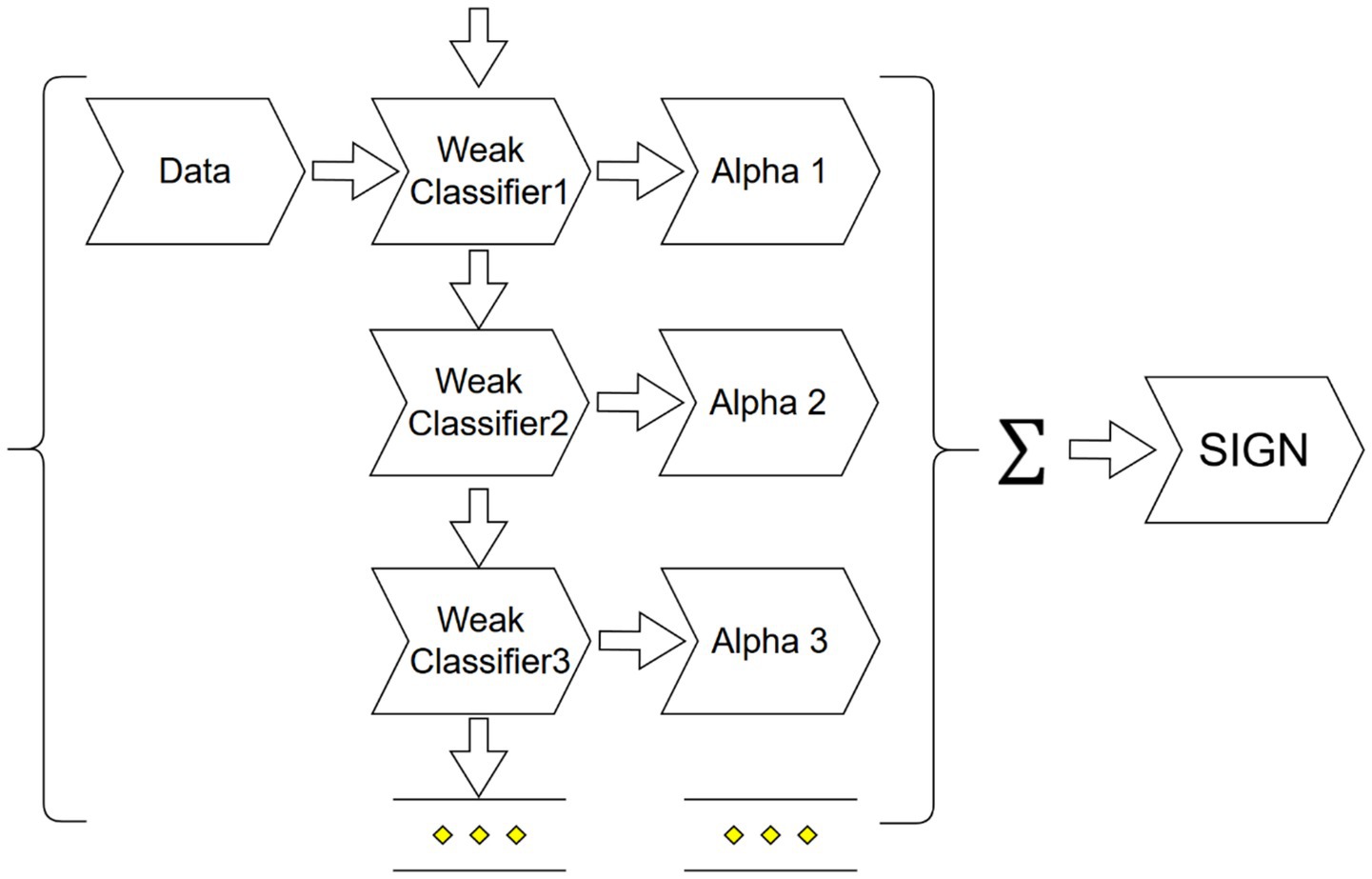
Figure 1. AdaBoost flowchart.

The operation process of AdaBoost is highly adaptive. Each round of training will dynamically adjust the weight of the sample according to the misclassification results of the previous round of the model, so that the subsequent weak learners will focus more on the samples that were previously mispredicted. The final prediction is obtained based on the weighted voting (for classification problems) or weighted average (for regression problems) of all weak learners. This study uses AdaBoost prediction, especially for high-dimensional and highly variable categories such as Scope 3 emissions, referring to the relevant empirical results of Serafeim and Velez Caicedo (2022). Compared with linear models, AdaBoost can capture more complex data structures and effectively enhance the model’s ability to identify abnormal patterns by correcting learning errors layer by layer. Estimation is specified as Equation 3 as below.

$\begin{array}{ll}{\alpha }_t=\frac{1}{2}ln\left(\frac{1-{\epsilon }_t}{{\epsilon }_t}\right)& (3)\end{array}$

3.1.4 XGBoost

The last machine learning approach used in this study is Extreme Gradient Boosting (XGBoost). Compared with traditional Boosting methods such as AdaBoost, the main difference of XGBoost lies in its optimization strategy; XGBoost builds the decision tree round by round for prediction correction, and the built-in regularization mechanisms (L1 and L2) of XGBoost help to control the complexity of the model and reduce the over-simulation risk, which makes it highly computationally efficient when applied to large datasets. The feature importance of XGBoost can further reveal the key variables and help provide model interpretation results. All models were tuned via GridSearchCV with five-fold cross-validation using RMSLE as the scoring metric (see Equation 4). The best parameter set from the search was used to train the final model on the training data. The formula and training flowchart of XGBoost is presented in Equation 4 and Figure 2:

$\begin{array}{ll}{g}_i=\frac{\partial L(y_i,{\widehat{y}}_i)}{\partial {\widehat{y}}_i},h_i=\frac{{\partial }^{2}L(y_i,{\widehat{y}}_i)}{\partial {\widehat{y}}_i^2}& (4)\end{array}$

Figure 2

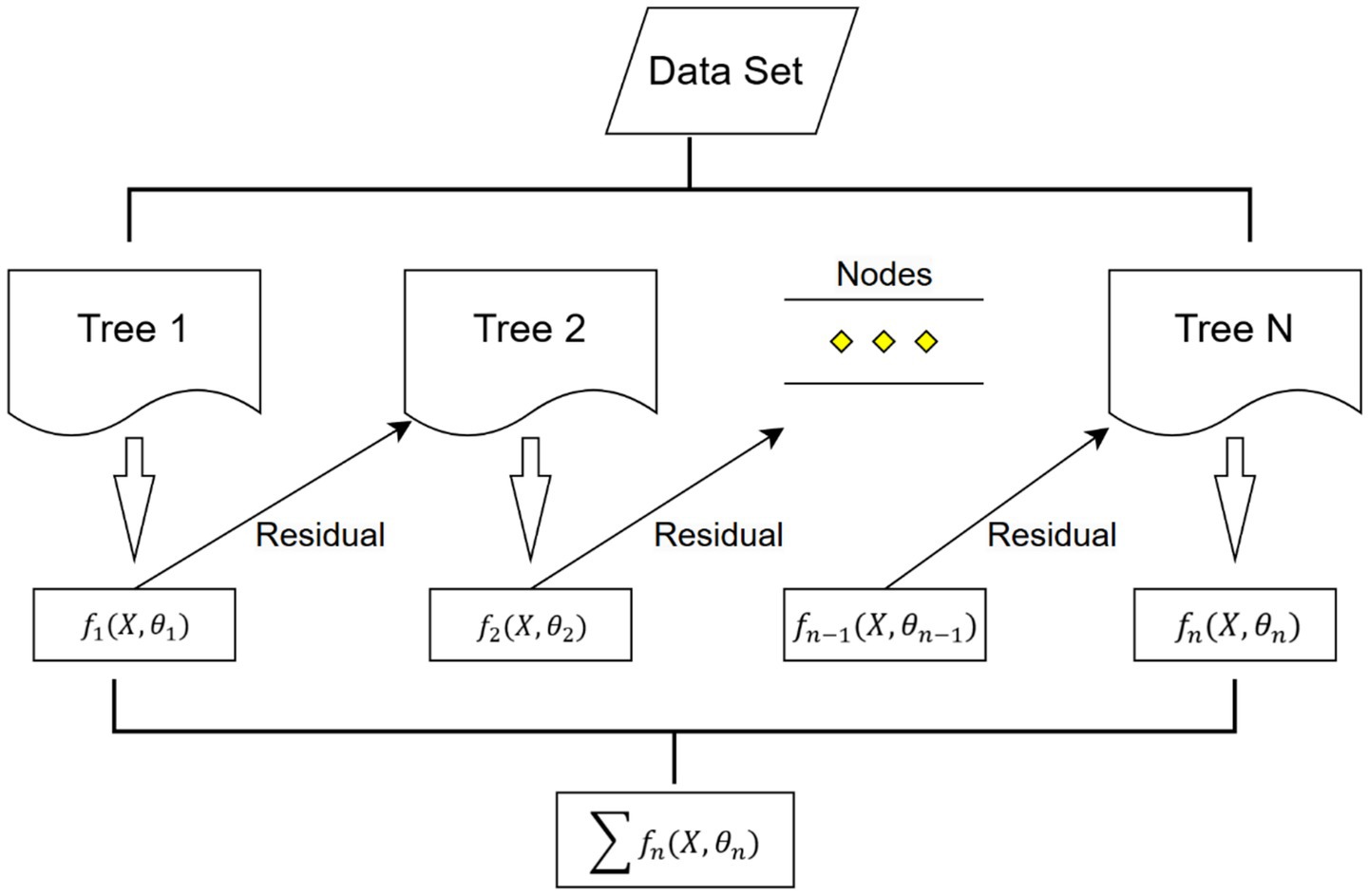
Figure 2. XGBoost flowchart.

3.2 Data and variable definitions

For analysis, we considered the relevant features of listed companies that might affect Scope 3 emissions. While more detailed data, such as company-specific historical energy usage, may be available but not used in this study, we focused on practical and commonly available indicators. The selected indicators can be divided into two main groups: One category specific to individual company and four additional categories typically available for most company categories. The first category includes essential characteristics of the company, for which we obtained financial feature data from the Taiwan Economic Journal (TEJ). The remaining four categories include accounting and financial statement variables, financial ratios, resource consumption data, and governance performance, which are standard across companies. Specifically, we included operational performance from the income statement and calculated financial ratios like profitability and operating efficiency. We also incorporated the company’s water consumption data and Taiwan-specific corporate governance evaluation performance. Lastly, to enhance the accuracy of Scope 3 carbon emissions prediction, we cross-referenced the available data with Scope 1 and Scope 2 emissions data collected from 2014 to 2023 and used for machine learning predictions. The variables used in the machine learning models were all numerical (e.g., financial indicators, water usage, sustainability performance), and no categorical variables such as industry codes or country codes were included. Consequently, no encoding procedures for categorical variables were required.

We provide the definitions and descriptive statistics of the selected variables in Tables 1, 2. In the following, we also present the rationale for including each variable in the model and explain their relevance to Scope 3 emissions.

Table 1

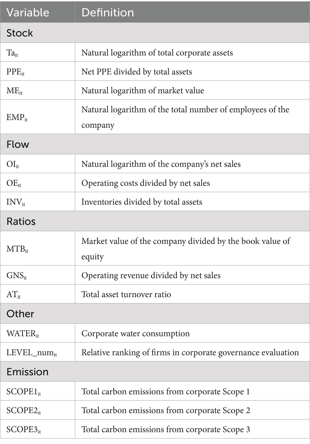
Table 1. Definition of selected variables.

Table 2

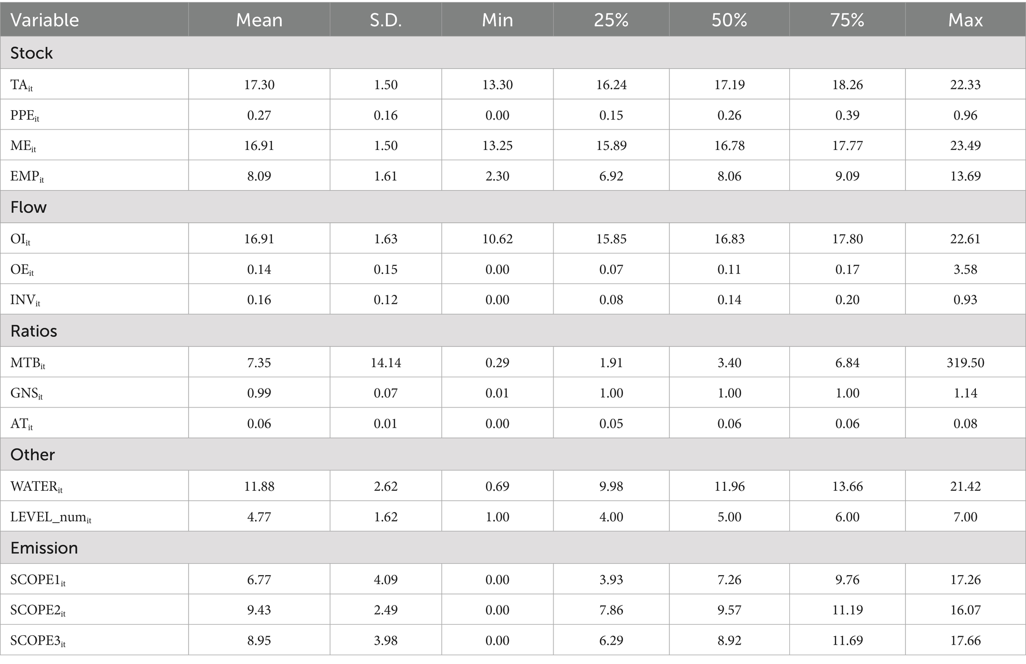
Table 2. Descriptive statistics of selected variables (N = 10,449).

Total assets reflect the overall scale of the firm’s operations and capital base. Larger firms (with more factories, equipment, etc.) tend to have larger supply chains and greater production capacity, which can lead to higher Scope 3 emissions. Asset-heavy companies (manufacturers, resource extraction, etc.) generally have more value-chain emissions than asset-light companies (e.g., software or service firms). Total assets have been used as a predictor in emissions models (Nguyen et al., 2021). Market Value is another measure of company size from an investor perspective. It captures not only the scale of the business but also intangible factors (brand, intellectual property, growth prospects). Prior research has included a “market valuation multiple” in prediction models for emissions (Cheema-Fox et al., 2021). Sales is a fundamental proxy for firm size and output, which in turn drives the scale of value-chain activities. Higher sales generally indicate a larger volume of products or services, often correlating with greater Scope 3. Prior studies commonly use revenue to estimate or scale emissions (Serafeim and Velez Caicedo, 2022). Operating Costs (or Cost of goods sold) reflect the quantity and value of materials, components, and services purchased. These upstream purchases directly generate Scope 3 emissions in supply chains (Category I: Purchased Goods and Services). It serves as a proxy for the volume of upstream economic activity. Recent models have explicitly incorporated COGS to improve Scope 3 predictions, given its direct connection to supply chain intensity (Nguyen et al., 2023; Nguyen et al., 2021). Inventory can indicate the scale of goods in production or storage, which in turn relates to supply chain throughput and manufacturing activity. Large inventories may reflect extensive production volume or procurement, implying substantial upstream Scope 3 emissions associated with producing those stored goods and raw materials. Previous study found inventory turnover to be a significant predictor for certain Scope 3 estimation (Serafeim and Velez Caicedo, 2022). Market-to-Book Ratio is a useful indicator of a firm’s business model and asset intensity. A high M/B ratio suggests that a company’s value derives largely from intangibles (brand, R&D, software, etc.) while a low M/B ratio may indicate a company with substantial tangible assets and possibly a commodity-like business (which often entails significant emissions). Asset turnover measures how efficiently a company uses its assets to generate sales. A high asset turnover means a company generates a lot of revenue with relatively few assets while a low asset turnover might signal a capital-intensive producer that does more in-house (potentially resulting in more Scope 1 and 2 emissions while somewhat lower Scope 3 proportionally). By including asset turnover, the model can detect such differences between a high-turnover company might be outsourcing emissions to suppliers (higher Category 1 emissions relative to its own Scope 1), whereas a low-turnover firm might internalize emissions (Serafeim and Velez Caicedo, 2022). Water Consumption is not a greenhouse gas metric per se, but it serves as a proxy for process intensity and industrial activity. High water consumption often signals that a company has energy-intensive cooling, processing, or agricultural operations that tend to entail significant GHG emissions. Furthermore, there is a direct linkage: treating and pumping large volumes of water requires substantial energy, which in turn produces CO₂ emissions. It’s estimated that each cubic meter of water delivered/treated can embed 10.5 kg of CO₂ emissions from the energy used (GRESB, 2025). By including water consumption data (available in TEJ’s dataset), the model captures an aspect of operational scale and process intensity not reflected in financials to get a more holistic view of impact. For example, if a company’s processes use extraordinary amounts of water, it likely engages in heavy manufacturing or resource processing that also drives up Scope 3 emissions upstream. Corporate governance score (as provided by TEJ) reflects the quality of a firm’s oversight, transparency, and management practices. Strong governance can influence Scope 3 emissions in that better governance and dedicated sustainability oversight are more likely to measure and manage their supply chain emissions. Including a governance score acts as a proxy for the firm’s likely commitment to managing value-chain impacts. Finally, the model incorporates the firm’s own direct (Scope 1) and energy-purchased (Scope 2) emissions. They are critical explanatory variables for Scope 3 due to the nature and scale of the company’s operations. Generally, a company with large Scope 1 and 2 emissions (e.g., semiconductor or steel sector) is engaged in energy-intensive processes, which often means it also has a carbon-intensive supply chain (high Scope 3 upstream from raw materials) and possibly carbon-intensive products. By including Scope 1 and 2 and a breadth of financial and operational variables, we try to balance the model. Scope 1 can serve as a proxy for downstream use-phase in some cases. Similarly, we included revenue (which correlates with downstream volume) and operating cost. This mix helps the model not lean entirely one way. These steps mitigate bias but cannot eliminate it completely. Without explicit product data, some downstream-heavy emissions may remain under-predicted. In conclusion, the selection of input variables critically influences whether a Scope 3 prediction model leans towards capturing upstream or downstream emissions. A well-rounded set of features (financial, operational, industry, etc.) can reduce bias, but data gaps (especially on downstream use) mean that some bias is unavoidable.

Despite the inclusion of a diverse set of financial and operational variables, this study is constrained by the availability of data within the Taiwan Economic Journal (TEJ). Specifically, several known drivers of Scope 3 emissions could not be incorporated due to lack of firm-level disclosure. These include (1) the number and characteristics of suppliers, (2) product use-phase emissions data, (3) transportation and logistics metrics such as distance shipped or freight mode, and (4) procurement expenditures by category. Prior literature has highlighted the relevance of these variables, especially for capturing downstream Scope 3 emissions, but such data are either proprietary or not publicly reported. As a result, our model relies on available proxies and may exhibit lower predictive accuracy for emissions categories that are highly dependent on these unobserved inputs. This limitation is consistent with challenges faced by other Scope 3 studies and underscores the need for improved corporate emissions transparency.

Given the constraints in variable availability, we process our data through rigorous steps designed to ensure data quality and representativeness. Our sample started from 76,513 company-years observations. 39,117 data were removed due to missing corporate governance assessments only commenced in 2014. An additional 26,947 data were excluded because of incomplete financial data, water consumption, or other critical missing values. The final dataset used for this study, included 10,449 company-years observations. All variables were compiled into a balanced panel dataset without missing values; thus, no imputation was necessary. Missing values occurred only in the target variable, which were predicted using the machine learning models.

3.3 Data preprocessing

All numerical features were first processed using polynomial feature expansion (degree = 2), which allowed the models to capture potential non-linear interactions between variables. The expanded feature set was then standardized to zero mean and unit variance using the StandardScaler in scikit-learn to ensure that all variables contributed equally to the model training. Outliers in the numerical variables (except governance ranking) were mitigated using Winsorization at the 1st and 99th percentiles. The dataset was subsequently split into training (80%) and test (20%) subsets using a fixed random seed to ensure reproducibility.

4 Empirical results

We report three different metrics to evaluate the predictive accuracy of the models. Given the characteristics and limitations of each metric, using multiple statistics to assess the models increases the robustness of our conclusions.

First, we report the Root Mean Squared Logarithmic Error (RMSLE) in Equation 5. Lower RMSLE values indicate lower percentage errors in predicted emissions. It is important to note that RMSLE penalizes underestimated predictions more than overestimated ones, making it practical for handling small and variable data points, such as Scope 3 emissions.

$\begin{array}{ll}\mathit{\text{RMLSE}}=\sqrt{\frac{1}{n}\sum _{i=1}^n{(log({\widehat{y}}_i+1)-log(y_i+1\left)\right)}^2}& (5)\end{array}$

$\begin{array}{ll}{R}^2=1-\frac{{\sum }_{i=1}^n{(y_i-{\widehat{y}}_i)}^2}{{\sum }_{i=1}^n{(y_i-\overline{y})}^2}& (6)\end{array}$

$\begin{array}{ll}\mathit{\text{MAPE}}=\frac{1}{N}\sum _{i=1}^N\frac{1}{T}\sum _{j=1}^T\frac{\mid P_{i,j,\mathit{\text{generic}}}-P_j\mid }{P_j}& (7)\end{array}$

Second, we report the R-squared (R²) between predicted and actual values in Equation 6. The R² value ranges from 0 to 1, with higher values indicating a more robust ability of the model to explain the variance in the target variable. However, R² primarily measures the explanatory power rather than prediction accuracy, showing how much of the variance is explained by the input features, but it does not directly reflect the magnitude of prediction errors (Chicco et al., 2021). To compensate for this limitation and provide a holistic assessment of predictive performance, we included additional metrics, specifically RMSLE and MAPE.

Third, we report the Mean Absolute Percentage Error (MAPE) for non-zero reported values in Equation 7. Lower MAPE values mean lower percentage errors. Generally, MAPE values below 10% are considered excellent, while values between 10 and 20% are acceptable, and values above 20% indicate more significant errors. Unlike RMSLE, MAPE penalizes overestimated predictions more heavily than underestimated ones because the errors are divided by the reported values, making it more sensitive to extremely high values.

The models are trained on a training set comprising 80% of the total samples. All reported prediction metrics are evaluated on a holdout test set, consisting of 20% of the total samples the model did not see. The data split between the training and test sets is initialized using a pseudorandom number generator with seed 1 to ensure the reproducibility and robustness of the results.

In the results presented in Tables 3, 4, we categorize our predictions primarily based on the nature of the target variable—specifically, whether the Scope 3 emissions data contain zero values or not. This distinction is crucial because zero values represent firms with either no reported Scope 3 emissions or potential data omissions, influencing the predictive accuracy and behavior of the models. With this consideration, Table 3 first provides the prediction results for the dataset that includes these zero values. Overall, we obtained model finesses of 82.28, 75.94, 57.24, and 81.27 under the four machine learning methods corresponding to the four prediction models: Random forest, K-NN, AdaBoost, and XGBoost. In addition to the overall firms, we also analyzed different industries, and we included the most developed industries in Taiwan today, as well as the green energy industry, which is essential for future sustainability. Our results show that the semiconductor industry, which is currently the most critical industry in Taiwan, has higher emissions than the other listed firms for all four machine learning methods. Among the other industries, we also find that the steel, communication networks, and electronic components industries have better forecasts than the overall firms.

Table 3

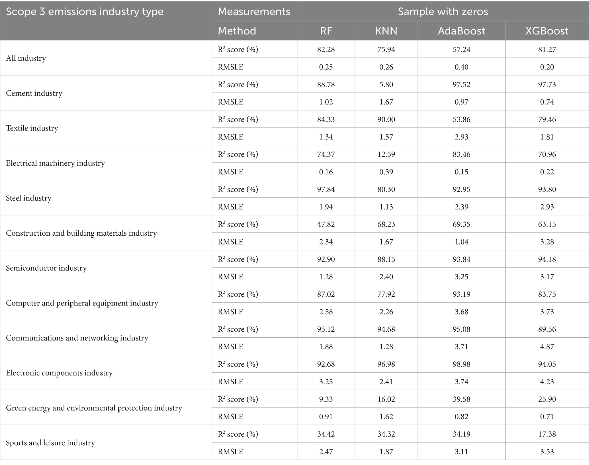
Table 3. Prediction results of 4 ML for with zero values.

Table 4

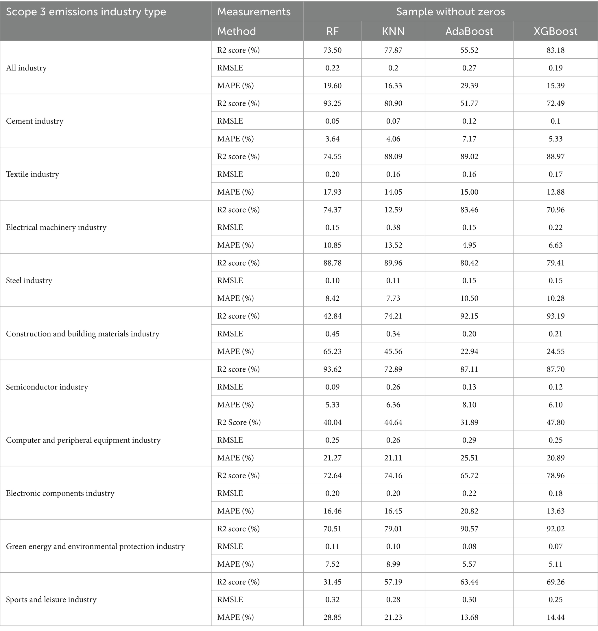
Table 4. Prediction results of 4 ML for with zero values.

In Table 4, we excluded the samples with Scope 3 emissions equal to 0 and reran the predictions. The R² values of the four prediction methods are 73.50, 77.87, 55.52, and 83.18%, respectively, with good model fit on average. This further supports the use of correlated variables for forecasting. In the prediction of individual industries, we find that the textile, iron, steel, and semiconductor industries show better prediction performance. These industries have been influential in Taiwan at different times and tend to have a more significant environmental impact, which may lead to better model fits and lower error values.

We present the prediction graphs for Scope 3 in Figures 3, 4 with and without zero, respectively. Our graphs present the forecast results for the overall firm. Specifically, our results in these graphs have similar predictive conclusions, with the predictive model results showing more spiky distributions, a greater concentration of predicted values around the mean, and fewer extreme values compared to the publicly available Scope 3 carbon emissions data. In addition, the distribution of the predicted data is more centered around the mean value, thus avoiding extreme values, than the results for Scope 3 emissions that contain zero.

Figure 3

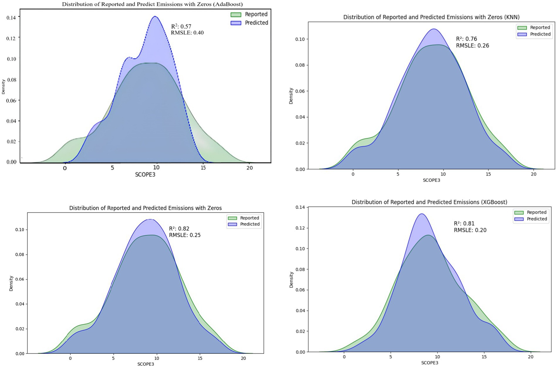
Figure 3. Four model predictions of Scope 3 including zero.

Figure 4

Figure 4. Four model predictions of Scope 3 excluding zero.

Table 5 presents in SHAP-based rankings, RF model shows a consistent reliance on SCOPE2-related variables, with all top 10 features involving SCOPE2 in either standalone or interaction form. KNN’s top features are dominated by interaction and squared terms (e.g., INV², EMP²), indicating a preference for non-linear transformations over raw variables. AdaBoost (ADA) is highly sensitive to SCOPE2*INV, with 14.98%. XGBoost (XG) displays the most concentrated dependence, with SCOPE2*AT (26.08%) and WATER*SCOPE2 (17.28%) jointly accounting for over 43% of total SHAP importance. Table 6 displays the permutation results. The RF sorts emission-related variables most important. KNN shows an evenly distributed importance profile (1.18%–1.23%), consistent with its distance-based nature. ADA reaffirms the dominance of SCOPE2-related variables. XG’s leading features—SCOPE2*AT, SCOPE2*INV, SCOPE2*PPE, and WATER*SCOPE2—closely mirror its SHAP rankings.

Table 5

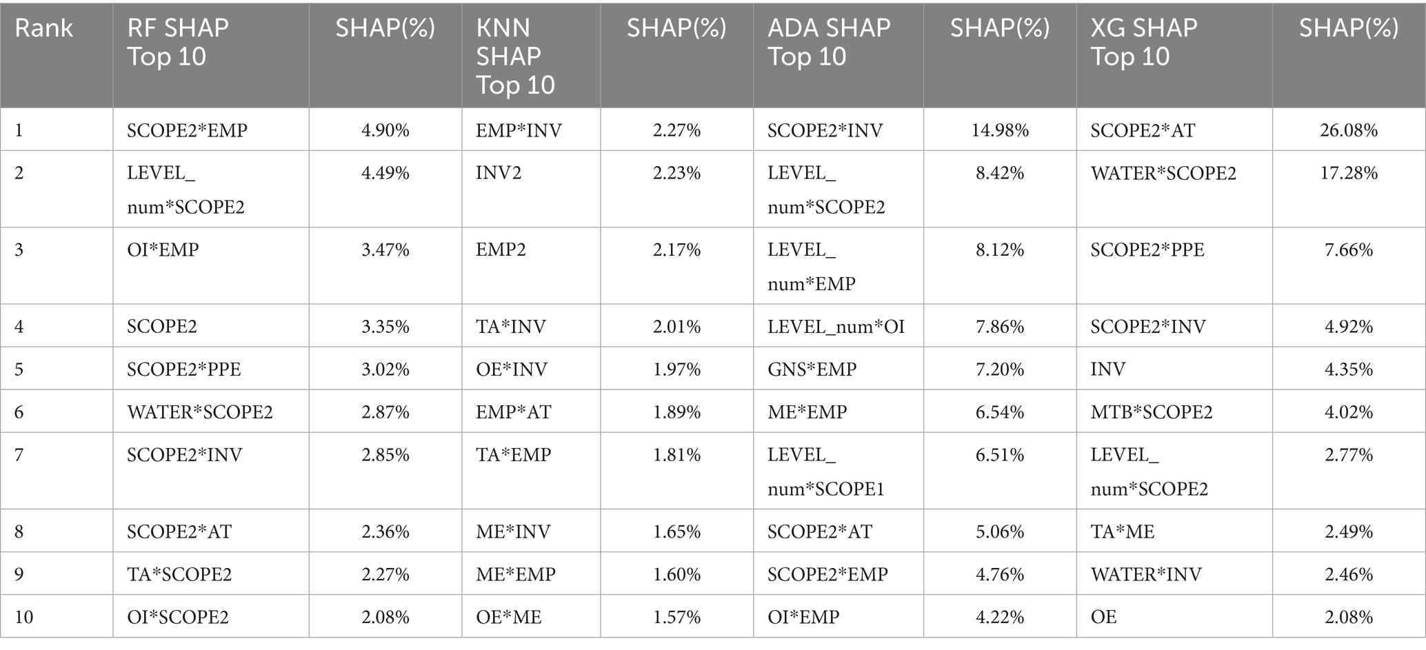
Table 5. SHAP% observations.

Table 6

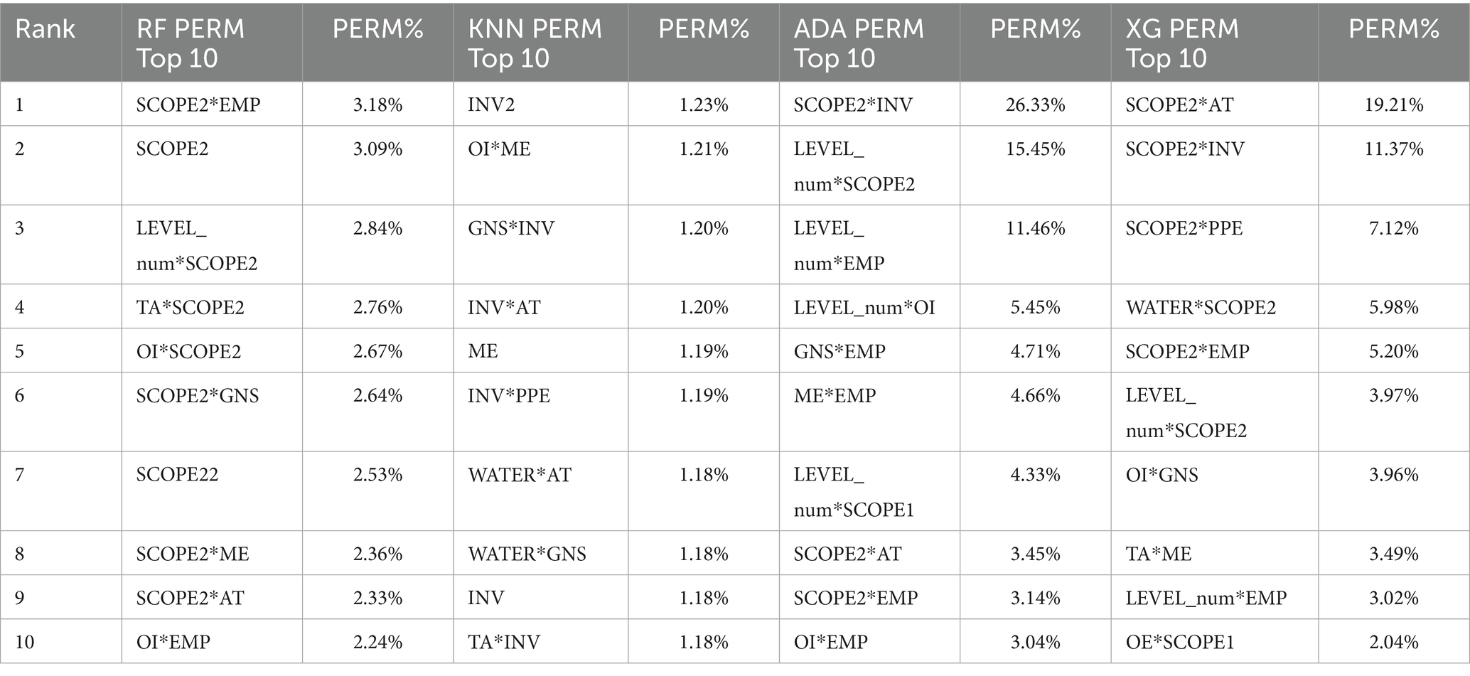
Table 6. PERM% observations.

5 Discussion

This study compared four machine learning algorithms—K-Nearest Neighbors, random Forest, AdaBoost, and XGBoost—to estimate Scope 3 greenhouse gas emissions using publicly available firm-level financial and operational data. Our results demonstrate that these machine learning approaches significantly outperform traditional linear regression techniques (Serafeim and Velez Caicedo, 2022). Specifically, AdaBoost achieved an average R-squared value of approximately 0.78, considerably exceeding the baseline linear regression model’s R-squared of about 0.46. Such an improvement underscores the capability of advanced algorithms to capture complex non-linearities overlooked by simpler regression methods, contributing notably to sustainable accounting scholarship (Magazzino and Mele, 2022; Nguyen et al., 2023).

A particularly innovative aspect of our approach is the integrated use of diverse data sources. Traditionally, Scope 3 estimations often rely on broad sector-average emission factors or economic input–output modeling techniques. In contrast, our method combines detailed firm-specific data, including Scope 1 and Scope 2 emissions, financial indicators (such as revenue, total assets, and operational expenditures), and industry classifications. This integrated approach leverages readily accessible financial and operational proxies to provide robust approximations of firms’ value-chain emissions, presenting a practical advance in Scope 3 carbon accounting. In the green energy sector, the relatively low R² may reflect the industry’s early-stage development in Taiwan, where many firms are supported by government subsidies and policy incentives. This setting leads to more volatile financial and operational metrics, weakening the model’s ability to capture stable relationships with Scope 3 emissions.

6 Conclusion and implications

Nevertheless, several limitations merit discussion. First, the quality and completeness of corporate reporting substantially constrains the precision of our estimates. Scope 3 disclosures often remain partial or inconsistent across categories, leaving considerable uncertainty around estimations for non-disclosing firms (Busch et al., 2022). Moreover, our reliance on aggregated firm-level proxies inherently misses granular differences within supply chains, such as individual supplier practices or specific product-level emission characteristics. While feature-importance analyses such as SHAP values and permutation importance were conducted for selected models, they were not exhaustively applied across all algorithms, which may limit comparability in interpretability results. Industry heterogeneity also presents challenges; while our models incorporate industry-level identifiers, the variability of emissions profiles and reporting standards across sectors suggests potential limitations in using a unified model for all firms. Finally, the current study is limited to Taiwan industries, so its generalizability is limited.

Recognizing these limitations opens clear avenues for future research. One valuable extension is to focus on more granular, category-level Scope 3 modeling. Prior work indicates that modeling individual emission categories separately—such as purchased goods, transportation, or business travel—can substantially improve the accuracy of total emission predictions (Khan and Kahn, 2020; Schmidt et al., 2022). Additionally, assessing model performance across different geographic contexts would further establish robustness and generalizability. Cross-national comparisons could help evaluate whether model adjustments are necessary to account for distinct economic and regulatory environments. Finally, sector-specific modeling approaches or hybrid techniques that integrate machine learning with engineering-based estimation methods may effectively address industry-specific emission drivers.

The implications of our findings extend to both scholarly research and corporate sustainability practice. Academically, this study highlights promising interdisciplinary intersections between environmental accounting and machine learning, encouraging further exploration into data-driven methods to overcome information gaps in emissions reporting. Practically, the developed models offer sustainability professionals a viable tool for approximating Scope 3 emissions without exhaustive direct supplier data. The interpretability features inherent in algorithms like random forest and XGBoost—such as feature importance analyses—can provide meaningful insights into emission drivers, helping prioritize areas for targeted emission-reduction interventions. Thus, combining advanced analytics with widely available corporate data can significantly enhance both the understanding and management of corporate carbon footprints.

Data availability statement

The data analyzed in this study was obtained from https://www.tejwin.com/. Requests to access these datasets should be directed to the corresponding author.

Author contributions

S-YW: Conceptualization, Writing – original draft, Writing – review & editing. N-ZY: Methodology, Formal analysis, Writing – original draft, Visualization.

Funding

The author(s) declare that no financial support was received for the research and/or publication of this article.

Conflict of interest

The authors declare that the research was conducted in the absence of any commercial or financial relationships that could be construed as a potential conflict of interest.

Generative AI statement

The authors declare that Gen AI was used in the creation of this manuscript. The authors declare the use of generative AI technology (GPT-4o) for formatting and arranging the references section of this manuscript. The authors carefully verified all references for accuracy and completeness and ensured compliance with Frontiers' guidelines.

Any alternative text (alt text) provided alongside figures in this article has been generated by Frontiers with the support of artificial intelligence and reasonable efforts have been made to ensure accuracy, including review by the authors wherever possible. If you identify any issues, please contact us.

Publisher’s note

All claims expressed in this article are solely those of the authors and do not necessarily represent those of their affiliated organizations, or those of the publisher, the editors and the reviewers. Any product that may be evaluated in this article, or claim that may be made by its manufacturer, is not guaranteed or endorsed by the publisher.

References

Aatola, P., Ollikainen, M., and Toppinen, A. (2013). Price determination in the EU ETS market: theory and econometric analysis with market fundamentals. Energy Econ. 36, 380–395. doi: 10.1016/j.eneco.2012.09.009

Crossref Full Text | Google Scholar

Bai, F. J. J. S. (2023). A machine learning approach for carbon dioxide and other emissions characteristics prediction in a low carbon biofuel-hydrogen dual fuel engine. Fuel 341:127578. doi: 10.1016/j.fuel.2023.127578

Crossref Full Text | Google Scholar

Bhatt, H., Davawala, M., Joshi, T., Shah, M., and Unnarkat, A. (2023). Forecasting and mitigation of global environmental carbon dioxide emission using machine learning techniques. Clean. Chem. Eng. 5:100095. doi: 10.1016/j.clce.2023.100095

Crossref Full Text | Google Scholar

Breiman, L. (2001). Random forests. Mach Learn 45, 5– 32.

Google Scholar

Busch, T., Johnson, M., and Pioch, T. (2022). Corporate carbon and climate data disclosure: challenges and developments in measuring, reporting, and verifying corporate greenhouse gas emissions. J. Bus. Ethics 179, 235–252. doi: 10.1111/jiec.13008

Crossref Full Text | Google Scholar

Çanakoğlu, E., Adıyeke, E., and Ağralı, S. (2018). Modeling of carbon credit prices using regime switching approach. J. Renew. Sustain. Energy 10:035901. doi: 10.1063/1.4996653

Crossref Full Text | Google Scholar

Carraro, C., and Favero, A. (2009). The economic and financial determinants of carbon prices. Finance Uver Czech J Econ. Finance 59, 426–439.

Google Scholar

Cheema-Fox, A., LaPerla, B. R., Serafeim, G., Turkington, D., and Wang, H. (2021). Decarbonizing everything. Financ. Anal. J. 77, 93–108. doi: 10.1080/0015198X.2021.1909943

Crossref Full Text | Google Scholar

Chevallier, J. (2013). Carbon price drivers: an updated literature review. Int. J. Appl. Logist. 4, 1–7. doi: 10.4018/ijal.2013100101

Crossref Full Text | Google Scholar

Chicco, D., Warrens, M. J., and Jurman, G. (2021). The coefficient of determination R-squared is more informative than SMAPE, MAE, MAPE, MSE and RMSE in regression analysis evaluation. Peer J. Comput. Sci. 7:e623. doi: 10.7717/peerj-cs.623

PubMed Abstract | Crossref Full Text | Google Scholar

Christiansen, A. C., Arvanitakis, A., Tangen, K., and Hasselknippe, H. (2005). Price determinants in the EU emissions trading scheme. Clim. Pol. 5, 15–30. doi: 10.1080/14693062.2005.9685538

Crossref Full Text | Google Scholar

de Oliveira, U. R., Menezes, R. P., and Fernandes, V. A. (2024). A systematic literature review on corporate sustainability: contributions, barriers, innovations and future possibilities. Environ. Dev. Sustain. 26, 3045–3079. doi: 10.1007/s10668-023-02933-7

Crossref Full Text | Google Scholar

Freund, Y., and Schapire, R. E. (1997). A decision-theoretic generalization of online learning and an application to boosting. J. Comput. Syst. Sci. 55, 119–139. doi: 10.1006/jcss.1997.1504

Crossref Full Text | Google Scholar

GRESB. (2025) Water conservation is critical to achieving decarbonization. Insights. Available online at: https://www.gresb.com/nl-en/ (Accessed 7 August 2025).

Google Scholar

Guðbrandsdóttir, N., and Haraldsson, Ó. (2011). Predicting the price of EU ETS carbon credits. Syst. Eng. Procedia 1, 481–489. doi: 10.1016/j.sepro.2011.08.070

Crossref Full Text | Google Scholar

Ho, T. K. (1995). Random decision forests. Proc 3rd Int Conf Document Analysis and Recognition. (ICDAR) :278– 282.

Google Scholar

Hsu, A. Y., and Kwan, A. (2020). The role of deep learning in estimating greenhouse gas emissions: a review. J. Clean. Prod. 280:124135. doi: 10.1016/j.jclepro.2020.124135

Crossref Full Text | Google Scholar

Huang, Y., Zhang, Y., and Wang, L. (2021). Machine learning approaches for estimating Scope 3 emissions: a systematic review. Environ. Sci. Technol. 55, 11834–11849. doi: 10.1021/acs.est.1c07376

Crossref Full Text | Google Scholar

Jain, A., Padmanaban, M., Hazra, J., Godbole, S., and Weldemariam, K. (2023). Scope 3 emission estimation using large language models. In: Proceedings of the ACM SIGKDD International Conference on Knowledge Discovery and Data Mining.

Google Scholar

Javanmard, M. E., and Ghaderi, S. F. (2022). A hybrid model with applying machine learning algorithms and optimization model to forecast greenhouse gas emissions with energy market data. Sustain. Cities Soc. 82:103886. doi: 10.1016/j.scs.2022.103886

Crossref Full Text | Google Scholar

Jha, R., Jha, R., and Islam, M. (2025). Forecasting US data center CO₂ emissions using AI models: emissions reduction strategies and policy recommendations. Front Sustain. 5:1507030. doi: 10.3389/frsus.2024.1507030

Crossref Full Text | Google Scholar

Khan, A., and Kahn, A. (2020). Scope 3 emissions in the supply chain: a review of literature and future directions. Sustainability 12:6102. doi: 10.3390/su12156102

Crossref Full Text | Google Scholar

Khurana, S., Saxena, S., Jain, S., and Dixit, A. (2021). Predictive modeling of engine emissions using machine learning: a review. Mater Today Proc 38, 280–284. doi: 10.1016/j.matpr.2020.07.204

Crossref Full Text | Google Scholar

Magazzino, C., and Mele, M. (2022). A new machine learning algorithm to explore the CO₂ emissions-energy use-economic growth trilemma. Ann. Oper. Res. 345:665–683. doi: 10.1007/s10479-022-04787-0

Crossref Full Text | Google Scholar

Natarajan, S. K., Shanmurthy, P., Arockiam, D., Balusamy, B., and Selvarajan, S. (2024). Optimized machine learning model for air quality index prediction in major cities in India. Sci. Rep. 14:6795. doi: 10.1038/s41598-024-54807-1

Crossref Full Text | Google Scholar

Nelson, T., Kelley, S., and Orton, F. (2012). A literature review of economic studies on carbon pricing and Australian wholesale electricity markets. Energy Policy 49, 217–224. doi: 10.1016/j.enpol.2012.05.075

Crossref Full Text | Google Scholar

Nguyen, Q., Diaz-Rainey, I., Kitto, A., McNeil, B. I., Pittman, N. A., and Zhang, R. (2023). Scope 3 emissions: data quality and machine learning prediction accuracy. PLoS Clim. 2:e0000208. doi: 10.1371/journal.pclm.0000208

Crossref Full Text | Google Scholar

Nguyen, Q., Diaz-Rainey, I., and Kuruppuarachchi, D. (2021). Predicting corporate carbon footprints for climate finance risk analyses: a machine learning approach. Energy Econ. 95:105129. doi: 10.1016/j.eneco.2021.105129

Crossref Full Text | Google Scholar

Schmidt, M., Nill, M., and Scholz, J. (2022). Determining the Scope 3 emissions of companies. Chem. Eng. Technol. 45, 1218–1230. doi: 10.1002/ceat.202200181

Crossref Full Text | Google Scholar

Serafeim, G., and Velez Caicedo, G. (2022). Machine learning models for prediction of Scope 3 carbon emissions. Harvard Business School Accounting and Management Unit Working Paper (22-080).

Google Scholar

Tang, J., Gong, R., Wang, H., and Liu, Y. (2023). Scenario analysis of transportation carbon emissions in China based on machine learning and deep neural network models. Environ. Res. Lett. 18:064018. doi: 10.1088/1748-9326/acd468

Crossref Full Text | Google Scholar

Valls-Val, K., and Bovea, M. D. (2021). Carbon footprint in higher education institutions: a literature review and prospects for future research. Clean Techn. Environ. Policy 23, 2523–2542. doi: 10.1007/s10098-021-02180-2

PubMed Abstract | Crossref Full Text | Google Scholar

Wang, Y., Hao, Y., Hou, Y., Quan, Q., and Li, Y. (2024). Optimizing Scope 3 emissions in the automotive manufacturing industry: a multidisciplinary approach. Carbon Res. 3:49. doi: 10.1007/s44246-024-00131-2

Crossref Full Text | Google Scholar

Wiedmann, T., and Minx, J. (2008). A definition of carbon footprint. Ecol. Econ. 64, 947–963. doi: 10.1016/j.ecolecon.2007.04.014

Crossref Full Text | Google Scholar

Yahşi, M., Çanakoğlu, E., and Ağralı, S. (2019). Carbon price forecasting models based on big data analytics. Carbon Manag. 10, 175–187. doi: 10.1080/17583004.2019.1568138

Crossref Full Text | Google Scholar

Zhang, Y., Liu, J., and Chen, X. (2022a). Innovations in carbon footprint estimation: a review of recent advances. Environ. Res. Lett. 17:033001. doi: 10.1088/1748-9326/abdf68

Crossref Full Text | Google Scholar

Zhang, Y., Liu, X., Lei, L., and Liu, L. (2022b). Estimating global anthropogenic CO₂ gridded emissions using a data-driven stacked random forest regression model. Remote Sens 14:3899. doi: 10.3390/rs14163899

Crossref Full Text | Google Scholar