Abstract
This study examines the sustainability of urban growth, described by patterns of environmental fitness. The main assumption is that resource use—energy, materials, electricity, water, fossil fuels, soil, and humans—describes growth patterns whose sustainability can be categorized according to environmental fitness, which is assessed by the availability of environmental resources (characteristics of the environment) and the adaptation of the city to this availability (characteristics of the built environment). The article offers an innovative perspective by proposing a model for categorizing the sustainability of urban growth based on environmental fitness, but also by providing a mean to understand the city as a process and the city as a satisfier of needs. The methodology comprises two parts: (1) creating a matrix of indicators of urban environmental fitness and (2) constructing an urban growth sustainability index. From this methodology, six patterns emerged: (i) Economizing growth: available resources with maximum urban adaptation; (ii) Weak growth: availability of resources with minimal urban adaptation; (iii) Efficient growth: availability of resources with appropriate urban adaptation; (iv) Deficient growth: availability of resources without urban adaptation; (v) Efficient growth and of investment: lack of resources with urban investment; and (vi) Deficient growth and of degradation: lack of resources with urban deterioration and wear. The finding of these sustainable urban growth patterns demonstrates the concrete application of environmental adaptation theories and an understanding of the global behavior of cities. The empirical results support the assertion that urban growth presents challenges and potentials in terms of reduction, of reuse, and recycling; of urban sprawl, urban renewal, redevelopment and infill growth, and the efficiency and maintenance of urban infrastructure as guidelines for urban sustainability.
1 Introduction
Urban growth can be described by the patterns, processes, and dynamics of how cities expand, densify, transform, and reconfigure over time as the consequence of changes and evolutions in human needs and the consequent demand for and supply of resources. The capacity of cities to meet these needs depends on both the availability of environmental resources and the efficiency and sufficiency of urban infrastructure to provide access to them. Given that all human activity influences the environment due to both resource consumption and waste generation, it’s useful to understand cities as open, dynamic systems where input and output flows of matter and energy might be in balance to allow their operation and continuity without damaging the system—the environment and the built environment. This approach to the city from a systems perspective is used to discuss the concept of sustainability anchored in the interaction of a population and the carrying capacity of its environment, which can be regarded as a system state that is mediated by specific structures (Ben-Eli, 2018). The research focus is on the sustainability of urban growth based on the description of patterns of environmental fitness.
In this study, urban growth will be described in dimensions of space, form, and time.
1.1 Urban growth spatial patterns (two dimensions).
Urban growth spatial patterns refer to the ways in which cities and urban areas expand and develop over time, as well as the spatial distribution of different land uses within urban areas. They are influenced by a variety of internal and external factors, and several types have been defined in the literature, which reflect how urbanization is affected by the physical geography, economic, social, and natural factors of individual cities. These patterns are characterized by both the continuity of growth and the starting point of growth. Shi et al. (2012) developed spatial rules to identify three types of urban growth (infilling, edge sprawl, and peripheral) in peri-urban areas of Lianyungang City, China, noting that the predominant type of urban growth was edge sprawl. Mou et al. (2018) explain that, in general, urban growth involves three different spatial patterns: edge expansion, outlying, and infilling. Edge expansion refers to the phenomenon of homocentric outspread, indicating a spatially subsequent expansion and extension of urban built-up areas. Outlying is characterized by the new urban lands occurring beyond developed areas. Infilling is introduced as developing the vacant land between established patches. Subasinghe (2019) explored urban growth patterns based on urban land classification and detected three main types of urban growth: infill, sprawl, and leapfrog. However, he noted that only recognizing three types of urban growth patterns may be insufficient due to the complexity of urban growth. Qian et al. (2019) investigated green space patterns in urban areas defined by three growth types: edge expansion, peripheral, and infill, finding significant differences in green space patterns among different urban growth types. And the combination, discontinuity, or change of them over time is common; for instance, the urban growth in Chennai was shown to exhibit a high level of sprawl in peri-urban regions while maintaining a tendency to form a single patch of clumped and simple-shaped growth at the core (Aithal and Ramachandra, 2016). On this basis, and in summary, spatial patterns and their characteristics are presented in Table 1.
Table 1
| Urban growth types | Spatial pattern | Land use characteristics | Infrastructure development |
Environmental impacts |
|---|---|---|---|---|
| Urban sprawl | Expansion of urban areas into low-density, typically suburban or rural areas. It often involves continuous outward growth without a defined center, resulting in the spread of development over a large geographic area. | Low-density residential and commercial development, large areas of single-family housing, shopping malls, and industrial parks spread out over a wide area. | Requires extensive infrastructure expansion, including roads, utilities, and services, to support the spread of development over a wide area. | Can lead to habitat fragmentation, loss of agricultural land, increased automobile dependency, air and water pollution, and degradation of natural landscapes. |
| Peripheral | The expansion of urban areas is primarily at the periphery or edges of existing urbanized areas. | Include a mix of land uses, often featuring large-scale residential subdivisions, shopping centers, and industrial parks on the outskirts of existing urban areas. | Requires the extension of infrastructure networks to accommodate new development at the periphery, which can be costly and inefficient. | This can result in habitat destruction, loss of green spaces, increased traffic congestion, and environmental degradation at the urban fringe. |
| Leapfrog development | Development occurs sporadically, skipping over areas between existing urbanized areas. This results in isolated pockets of development separated by undeveloped or rural land. | Development occurs in patches or clusters with mixed land uses and varying densities. It may include residential, commercial, and industrial development but lacks continuity. | Infrastructure development may be less efficient as services need to be extended over large distances to reach isolated pockets of development. | Similar environmental impacts to urban sprawl may also result in additional pressure on undeveloped or rural areas located between urbanized patches. |
| Infilling growth | Development or redevelopment of vacant or underutilized land within existing urban areas, usually in densely populated areas or areas with existing infrastructure. | Typically, it involves intensification of land use within existing urban areas, including the construction of multifamily housing, mixed-use developments, and redevelopment of brownfield sites. | It could take advantage of existing infrastructure networks, reducing the need for costly new infrastructure development. However, upgrades or modifications to existing infrastructure may be necessary to accommodate increased density. | It is considered more environmentally sustainable compared to urban sprawl and leapfrog development since it utilizes existing infrastructure, reduces land consumption, and promotes compact, walkable communities. |
Types of urban growth spatial patterns and characteristics.
1.2 Urban form growth patterns (three dimensions)
Urban form considers physical and non-physical structures, the functionality, livability, social dynamics, and dimension of the built environment expansion shaped by historical, cultural, economic, geographic, planning, and political factors, among other factors. Describe aspects/characteristics of a city, such as the size and configuration of an urban area or its parts. It refers to how a city is understood, structured, or analyzed according to scale (Živković, 2020). Urban form is the result of human self-organization that follows diverse logics over time and is described qualitatively, quantitatively, or spatially at different scales and, in many cases, through isolated one-dimensional measurements. Urban form indicators provide valuable insights into the physical layout, structure, and spatial characteristics of urban growth. Density, land use mix, street network connectivity, building density, and green space availability, among others. Rather than referring to differences in population density or development, it is common to examine development patterns on the landscape when modeling urban growth; landscape metrics began to be used to analyze urban land use patterns, demonstrating significant changes in metropolitan areas, especially in more recently developed areas like certain Spanish metropolitan areas (Aguilera et al., 2011). Studies started to focus on the visualization of urban growth using geoinformatics and spatial metrics, for instance, the urban growth in Chennai was shown to exhibit a high level of sprawl in peri-urban regions while maintaining a tendency to form a single patch of clumped and simple-shaped growth at the core (Aithal and Ramachandra, 2016). In global datasets to characterize urban growth in both two- and three-dimensional forms across major cities worldwide, a variety of urban growth typologies were identified, such as outward, mature upward, budding outward, and combinations theories (Mahtta et al., 2019). Figure 1 shows a schematization of the scales for studying and understanding the city and its dimensions.
Figure 1

Urban form. Scales and dimensions.
1.3 Temporal patterns (four dimensions)
Urban growth over time involves change and evolves across different time periods, stages of development, phases of growth, and historical events that shape the city’s evolution and encompass long-term trends, short-term fluctuations, and cyclical patterns of urban change. The rate of growth indicates the rate at which the city changes over a given period; it may be constant, variable, or dependent on a variety of factors. Fenta et al. (2017) assessed the dynamics and spatial pattern of urban sprawl in Mekelle City, Ethiopia, using multitemporal Landsat imagery and found that the predominant urban sprawl was the extension of existing urban areas.
Different spatial or urban form growth patterns can vary in speed rate and explain different phenomena. Bagan and Yamagata (2012) investigated the dynamics of urban growth in Tokyo, Japan, combining Landsat imagery and census data, showing rapid urban expansion accompanied by a decrease in population density in the city center. The rate of growth provides critical information about the pace, extent, and way urban areas are expanding. By projecting growth rates, decisions can be made about where to allocate resources for essential services, determine appropriate land use patterns, and guide efforts to balance development with environmental protection and preservation. In Beijing’s rapid urban expansion process, significant urban growth has been observed on the fringe, especially in low-density gated communities and industrial development. As a result, the need for long-distance travel to external areas and the use of private vehicles on the city fringe have increased (Mou et al., 2018). Urban growth rates also reflect economic vitality and investment attractiveness, employment opportunities, and impacts on housing demand and values; assess infrastructure and service capacity; and support efforts to improve urban resilience by identifying vulnerabilities and planning for future challenges, such as climate change impacts.
1.4 Environmental fitness
Environmental fitness refers to the ability of an organism to survive and reproduce in a specific environment and, at the same time, the capacity of an ecosystem or environment to support and sustain diverse forms of life. In the context of this research, “environmental fitness” refers to the ability of an urban environment to maintain its ecological balance and provide a suitable place for human life in terms of health and wellbeing. Henderson’s book, “The fitness of the environment,” states that a fit environment can be defined as one in which the greatest consumer needs are met by the same environment, which means that the organism has less adaptive work to do. “The fitness of the environment” is one part of a reciprocal relationship, the fitness of the organism being the other. And the fitness of the environment is the result of characteristics which constitute a series of maxima so numerous, so varied, and so nearly complete among all the things involved in the problem that together they certainly form the greatest possible fitness (The University of Chicago Press, 2016). This relationship between the environment and the organism that inhabits it was studied by McHarg. In “Design with Nature,” Ian L. McHarg developed an ecological planning theory and method for analyzing and evaluating biophysical and sociocultural landscape characteristics to determine appropriate land uses. His suitability analysis method links planning and design to ecology and evolutionary biology with concepts such as energy, order and disorder, adaptation, health, creativity, and human agency, as well as his parallel constructs: syntropic fitness-health and entropic mismatches-morbidity and death (Bryant and Turner, 2019). Yang and Li (2019) conclude that McHarg is a forerunner in landscape performance evaluation. Through blending project goals and performance goals, McHarg’s method improves project performance and increases the validity of ecological planning (Figure 2). “Environmental fitness” is a systemic relationship between the environment and the city that could be valued through (a) the availability of environmental resources (characteristics of the environment) and (b) the adaptation of the city to this availability (characteristics of the built environment).
Figure 2
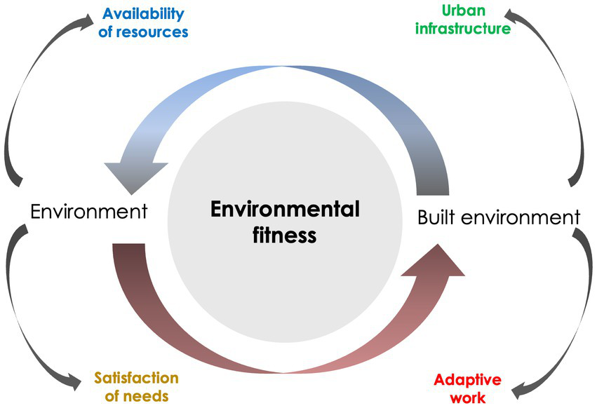
Environmental fitness.
The adequacy or balance between the environment and built environment is structured through the concept of fitness, which refers to the quality of following a path of interdependence, creating closed-loop systems where materials flow, helping to conserve resources, and reducing the negative impacts of linear “take-make-dispose” models of production and consumption. The urban system is a set of interconnected and interdependent elements that work together to achieve a specific goal within a physical or conceptual boundary that separates them from the broader environment in which they operate. Both the availability of environmental resources and the adaptation of the city to this availability of resources have limits defined by maximum and minimum values. Therefore, being a relationship between these two variables, the environmental fitness is also limited by a maximum and minimum value, defining a range of environmental fitness. In the following examples (
Figure 3), the environmental fitness of a city is represented by the height of each diagram.
Blue: the range of adaptation of the city to the environment.
Red: the city’s level of adaptation to the environment.
Green: the investment to achieve its maximum level of adaptation to the environment.
Yellow: system improvement limit.
Figure 3
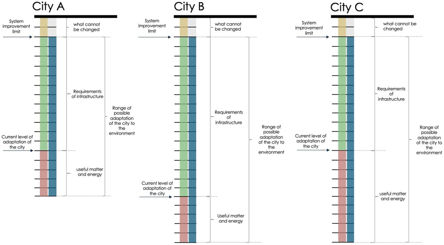
Example of environmental fitness in three hypothetical cities.
Two cities (A and B) have the same level of adaptation to the environment, but different ranges of environmental fitness. Therefore, the investment of the cities to achieve their maximum level of adaptation to the environment will be different.
Two cities (B and C) have the same range of environmental fitness but different levels of adaptation to the environment. Therefore, the investment of the cities to achieve their maximum level of adaptation to the environment will also be different.
Two cities (A and C) have different levels of adaptation to the environment and different ranges of environmental fitness. But in this case, the investment of the cities to achieve their maximum level of adaptation to the environment would be the same.
Cities A, B, and C have the same system improvement limit, so the dimension of what cannot be changed is the same.
A city is a manifestation of the actions of human beings in the artificial environment controlled by the measure of individual and social human needs. Batty and Marshall (2009) assert that cities are not a place or a space, or structures in space, but a set of networks where locations naturally emerge—the nodes in a network of complex relationships—and this explains why cities are understood as places that emerge out of a relational process that arises from the interaction of flows. Therefore, cities are regulated by interactions, feedback, and fitness between nature and human society, culture, economics, technology, and politics, all of which create an environment that can influence and be influenced by both ecological and evolutionary processes (Des Roches et al., 2021). Based on this interpretation, the space-form-time properties of complex systems, particularly those of a city, arise spontaneously from interactions between the elements that make it up and on time scales considerably larger than the scales on which the said interactions occur. Although the study of urban interactions is mainly conducted based on the interactions of geographical elements or spatial relations, in the context of globalization and production fragmentation, other flows, such as information flows, have explicit geographical meaning (Li and Duan, 2020).
The city can be described as a complex adaptive system, with interconnected and interacting elements that can learn, adapt, and self-organize, evolving based on feedback and interactions with each other and their environment. Cities, as complex systems, are characterized by a variety of interrelated elements and relationships between them that are not always apparent (Opromolla and Volpi, 2020). Systems have inputs of information or resources from the external environment, process or transform these inputs, and then generate results or outputs that are sent back to the environment. A closed-loop system is a type of system in which the output or result of the process is used to influence the input of the same system, creating a feedback loop. In this type of system, information about the output is compared to a reference or desired value, and any difference between the actual output and the reference is used to adjust and control the input. The concept of a closed-loop system is primarily used in control theory and engineering to describe a type of control mechanism.
According to Moore and Hague (2019), characteristics of systems are: (a) they have a purpose that defines them as a discrete entity and that provides the integrity that holds them together, the purpose is a property of the system as a whole and not of any of the parts; (b) the order in which the parts are arranged affects the performance of a system, if the components of a collection can be combined in any random order, then they do not form a system; and (c) systems attempt to maintain stability through feedback, which is the sending and returning of information that lets the system know how it is doing relative to some desired state. Sustainable development is a development model that highlights the relationship between man and nature that enables actual societies to satisfy their current and future needs, maintain their quality of life, and preserve and restore natural resources (Schipper and Meyers, 1992). It involves balancing economic, social, and environmental dimensions to ensure long-term wellbeing. From a system perspective, sustainability can be understood as the search for, construction of, or regeneration of circular and closed-loop systems that can make their own decisions and adapt automatically based on the feedback they receive.
The environmental fitness is a closed-loop system where the output influences the input in such a way as to maintain a desired state or set of conditions. Energy, matter, and processes are interlinked and interact, so changes in one affect the others. If they were recycled, reused, or improved and kept in use for as long as possible, waste generation would be minimized, resulting in greater economic efficiency, less pressure on ecosystems, and greater resilience to environmental and social challenges. The characteristics of closed-loop systems and how they relate to sustainability can be described as follows:
Feedback is used to monitor resource use, waste generation, and environmental impact.
Self-regulation is the capacity to adjust internal operations and behaviors in response to external or internal changes.
Dynamic response is the ability to respond to changes in the environment or resource availability.
The controller may be a management protocol, or a system designed to optimize resource use.
Error detection and correction are employed to identify areas where resources are being wasted or if the environmental impact is higher than desired.
Reduced sensitivity to external disturbances and internal variation.
Avoidance of forms of system instability, such as resource depletion or environmental degradation.
Environmental fitness is proposed as a systemic approach of sustainability in urban growth patterns that explores ways to develop closed-loop urban systems. The methodology comprises two parts: (1) creating a matrix of indicators of urban environmental fitness and (2) constructing an urban growth sustainability index.
2 Methodology
The methodology for defining urban growth sustainability patterns based on environmental fitness comprises two parts: (1) creating a matrix of urban environmental fitness and (2) constructing an index for urban growth sustainability.
2.1 Part 1: matrix of urban environmental fitness
The matrix is a set of indicators organized in a structure that represents the city as a closed-loop system. Based on the concept of fitness, resources were analyzed as flows with inputs, outputs, and recovery of resources (energy, materials, electricity, water, fossil fuels, minerals, biomass, and soil), as well as their influence on critical attributes (urban footprint, governance, social patterns, urban work, sustainability, waste, and transport; Table 2).
Table 2
| Resources | Critical attributes |
|---|---|
| 1. Total energy | A. Urban footprint: urban infrastructure and density |
| 2. Total materials | B. Governance: organizations and standards |
| 3. Electricity | C. Social patterns: the distribution of social groups |
| 4. Water | D. Urban work |
| 5. Fossil fuels | E. Global indicators: urban sustainability |
| 6. Construction minerals | F. Waste |
| 7. Biomass | G. Transport |
| 8. Soil | |
| 9. Human |
Indicator matrix attributes.
This arrangement provides a summary of information about the behaviors of the city in the aspects analyzed, as well as its structure. This could be useful for comparing it with another matrix of the same city at a different time or with another city within the same timeframe. It could help identify those indicators that are not available in direct sources but can be obtained from the geographical analysis on different scales, as well as those that can be represented geographically by sectors or districts rather than the type of data aggregation. Furthermore, the matrix arrangement facilitated the identification of critical attributes of a resource or a critical aspect within a resource flow, which in turn proved useful in defining areas for improvement in the management of resources and infrastructure. Indicators in vectors permit the analysis of a city as both a process and a satisfier.
When reading horizontally, inputs and outputs of matter and energy will be defined, as well as the matter and energy through different urban processes (the city as a process). Ideally, in a fully environmentally fit city, outflows or waste would be returned as inflows. These indicators are represented in the last column of the matrix (Table 3).
Table 3
| Inputs | A. Infrastructure | B. Per city | C. Per district | D. Per capita | E. Agriculture | F. Industrial | G. Comercial | H. Public services | I. Residential | J. Economical/production | K. Programs | L. Outputs (emission/waste) | M. Material or energy reused/recycled |
|---|---|---|---|---|---|---|---|---|---|---|---|---|---|
| 1. Total energy | Energy consumption and management | ||||||||||||
| 2. Materials | Material consumption and management | ||||||||||||
| 3. Electricity | Electricity consumption and management | ||||||||||||
| 4. Water | Water consumption and management | ||||||||||||
| 5. Fossil fuels | Air management | ||||||||||||
| 6. Fossil fuels | Fossil fuel consumption and management | ||||||||||||
| 7. Biomass | Biomass consumption and management | ||||||||||||
| 8. Soil | Soil consumption and management | ||||||||||||
| 9. Human | Lifestyle related to urban structure, infrastructure, and services | ||||||||||||
Summary information inputs/outputs.
When reading vertically, the city is understood as a satisfier insofar as its purpose is to ensure the features of urban structures and services (the city as a satisfier). Ideally, in a fully efficient city, resources would be allocated to provide its inhabitants with a high standard of living. These indicators can be found in the last row of the matrix (Table 4).
Table 4
| inputs | A. Infrastructure | Indicators by scale | E. Agriculture | F. Industrial | G. Comercial | H. Public services | I. esidential | J. Economical/production | K. Programs | L. Outputs (emissions/waste) | M. Material or energy reused/recycled | ||
|---|---|---|---|---|---|---|---|---|---|---|---|---|---|
| B. Per city | C. Per district | D. Per capita | |||||||||||
| 1. Total energy | Features of urban transport services | Features of urban infrastructure services | Economic urban investment | Urban quality (consumption metrics) | Environmental responsability | Carbon footprint and waste | Sustainable management | ||||||
| 2. Materials | |||||||||||||
| 3. Electricity | |||||||||||||
| 4. Water | |||||||||||||
| 5. Air | |||||||||||||
| 6. Fossil fuels | |||||||||||||
| 7. Bomass | |||||||||||||
| 8. Soil | |||||||||||||
| 9. Human | |||||||||||||
Summary information as urban structures.
The selection of indicators was based on three criteria: firstly, a comprehensive and accurate assessment of relevant environmental, economic, and social factors; secondly, the consideration of temporal and spatial horizons; and thirdly, the availability of pertinent information.
The usefulness of these indicators is enhanced by their capacity to monitor and assess the state of the environment by considering a manageable number of variables or characteristics.
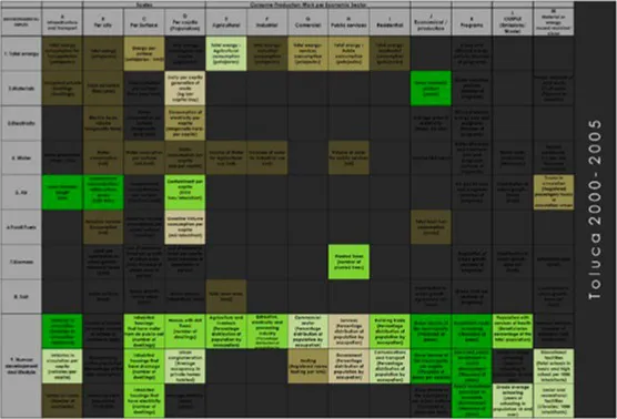
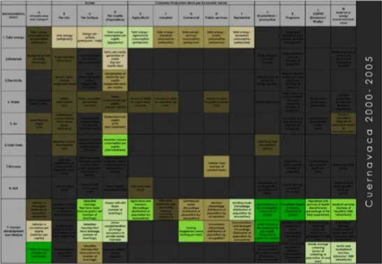
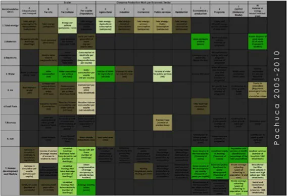
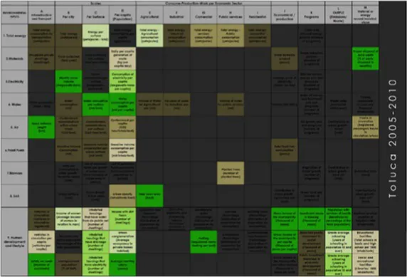
Their utility is further enhanced by their ability to identify relative changes in the availability of environmental resources and the adaptation of the city to the state of the environment, which can inform decision-making and drive action. For this reason, a set of indicators was organized and structured into indicator subsets that correspond to information from subsystems, as well as input and output types for each of the environmental, economic, and social resources. From this organization, particular analysis was carried out for every city, subsystem, time, space, and type of resource to generate efficiency scores for each type of characterized urban growth pattern (Table 5).
Table 5
| Scales | Consume production work per economic sector | ||||||||||||
|---|---|---|---|---|---|---|---|---|---|---|---|---|---|
| Environmental inputs | A. Infrastructure and transport | B. Per city | C. Per surface | D. Per capita (population) | E. Agricultural | F. Industrial | G. Comercial | H. Public services | I. Residential | J. Economical/production | K. Programs | L. Output (emissions/waste) | M. Material or energy reused/recycled/cleaned |
| 1. Total energy | Total energy consumption for transportation (petajoules) | Total energy (petajoules) | Energy per Surface (petajoules/km2) | Total energy consumption per capita (gigajoules) | Total energy consumption per capita (gigajoules) | Total energy industrial consumption (petajoules) | Total energy service consumption (petajoules) | Total energy consumption (petajoules) | Total energy residential consumption (petajoules) | Clean and efficient energy policies (number of programs) | |||
| 2. Materials | Occupied private dwellings (dwellings) | Trash collected (tons/year) | Trash collected per surface (tons/year/km2) | Daily per capita generation of waste (kg/per capita/day) | Waste reduction policies (number of programs) | Proper disposal of solid waste (percentage of waste disposed in landscape) | |||||||
| 3. Electricity | Electric sales volume (mW/h) | Power consumption per surface (megawatts-hour/km2) | Consumption of electricity per capita (Megawatts-hour-per capita) | Average price of electricity (pesos/kW-hour) | Efficient electric energy acts and programs (number of programs) | ||||||||
| 4. Water | Water production (mm3/año) | Water consumption (m3) | Water consumption per surface (m3/km2) | Water consumption per capita (m3per capita) | Volume of water for agricultural use (m3) | Volume of water for industrial use (m3) | Volume of water for public services (m3) | Income (M$/year) | Water efficiency and treatment acts and programs (number of programs) |
Wastewater production (mm3/year) | Treated wastewater (l/s per 1,000 inhabitants) | ||
| 5. Air | Road network length (km) | Contaminant concentrations within urban areas (CO2 tons) | Contaminant concentrations per surface (CO2-tons/km2) | Contaminant per capita (CO2 tons/inhabitant) | Air quality acts and programs (number of programs) |
Contribution to urban growth forest (km2) | Trucks in circulation (registered passenger trucks in circulation/urban surface) | ||||||
| 6. Fossil fuels | Gasoline volume consumption (m3) | Gasoline volume consumption per urban surface (m3/km2) | Gasoline volume consumption per capita (m3/inhabitant) | Total fossil fuel consumption (pesos) | |||||||||
| 7. Biomass | Land use contribution to urban growth—perennial forest (km2) | Loss of perennial forest per growth of urban area (km2/increase of urban area in period) | Lost of perennial forest per capita (km2/increase of population in period) | Planted trees (number of planted trees) |
Regulation of urban growth (number of programs) | Contribution to urban growth—bare soil (km2) | Reforested area (km2) | ||||||
| 8. Soil | Urban surface (km2) | Urban growth in 5 years (km2) | Urban density (inhabitants/km2) | Total sown area (km2) | Contribution to urban growth—agriculture soil (km2) | Green land use (number of programs) |
Contribution to urban growth—bare soil (km2) |
||||||
| 9. Human development and lifestyle | Vehicles in circulation (vehicles in circulation registered) | Income of women (average income of women in relation to men) | Inhabited housing that has water from the public net (number of dwellings) | Houses with dirt floors (number of dwellings) | Agriculture and livestock (percentage distribution of population by occupation) | Extractive, electricity, and processing industries (percentage distribution of population by occupation) | Commercial sector (percentage distribution of population by occupation) | Services (percentage distribution of population by occupation) | Building trade (percentage distribution of population by occupation) | Gross income of the municipality (1,000 pesos) | Investment made in housing (1,000 pesos) | Population with services of health (beneficiaries percentage of the total population) | Medical services (number of hospitals/1,000 inhabitants) |
| Vehicles in circulation per capita (vehicles/per capita) | Economically active population (percentage of the total population) | Inhabited housing that has drainage (number of dwellings) | Urban conglomeration (average occupancy in private homes habited) | Hosting (registered rooms per km2) | Government (percentage distribution of population by occupation) | Communications and transport (percentage distribution of population by occupation) | Gross income of the municipality per capita (1,000 pesos per capita) | Exercised public investment in social development (1,000 pesos) | Grade average schooling (years of schooling in population 15 and over) | Educational facilities (total schools in basic and high schools per 1,000 inhabitants) | |||
| Safety on roads (number of accidents) | Unemployment population (percentage of EAP) | Inhabited housing that has electricity from the public net (number of dwellings) | Average monthly salary (pesos) | Gross income of the municipality per urban surface (1,000 pesos per km2) | Public investment exercised in economic development (1,000 pesos) | Doctors (number of doctors per 1,000 inhabitants) | Social and recreational facilities (libraries/1,000 inhabitants) | ||||||
Matrix of urban environmental fitness.
The description, units, and sources of the selected indicators are shown in Table 6.
Table 6
| Indicator | Unit | Source | |
|---|---|---|---|
| 1. Total energy | |||
| 1A | Total energy | petajoules | Estimation based on data from SENER and population |
| 1B | Energy per surface | petajoules/km2 | Estimation based on data from SENER and urban surface |
| 1C | Total energy consumption per capita | gigajoules | Estimation based on data from SENER and population |
| 1E | Total energy consumption in agricultural sectors | petajoules | Estimation based on data from SENER and population |
| 1F | Total energy consumption in industrial sectors | petajoules | Estimation based on data from SENER and population |
| 1G | Total energy consumption in commercial sectors | petajoules | Estimation based on data from SENER and population |
| 1H | Total energy consumption in public sectors | petajoules | Estimation based on data from SENER and population |
| 1I | Total energy consumption in residential sectors | petajoules | Estimation based on data from SENER and population |
| 1 K | Clean and efficient energy policies | Number of programs | Number of programs for clean and efficient energy |
| 2. Materials | |||
| 2A | Total extraction of materials (tons) | Tons/year | SEMARNAT |
| 2B | Extraction of materials per surface (tons) | Tons-year/km2 | SEMARNAT |
| 2C | Extraction of materials per capita (tons) | kg/hab/day | SEMARNAT |
| 2D | Extraction of construction materials (tons) | Tons/year | SEMARNAT |
| 2 J | Materials productivity (pesos) | Pesos/tons | SEMARNAT |
| 2 K | Material efficiency | Number of programs | SEMARNAT |
| 2 M | Waste recycling | Percentage of waste recycled | INEGI |
| 3. Electricity | |||
| 3B | Power consumption per surface | Megawatts-hour/km2 | Electric sales volume/surface |
| 3C | Consumption of electricity per capita | Megawatts-hour-per capita | Electric sales (megawatts-hour)/electric energy users |
| 3D | Electricity consumption for transportation | Megawatt hour | U.S. Energy Information Administration |
| 3 J | Average price of electricity | Pesos/kW-hour | Comisión Federal de Electricidad (CFE) |
| 3 K | Efficient electric energy acts and programs | Number of programs | Author |
| 4. Water | |||
| 4A | Water production | mm3/year | Gestión del agua en las ciudades en México, Consejo Consultivo del Agua., 2010 |
| 4B | Water consumption | m3 | Estimation of water consumption per capita and population |
| 4C | Water consumption per surface | m3/km2 | Estimation from water consumption and surface |
| 4D | Water consumption per capita | m3per capita/year | National Commission of Water (CONAGUA) |
| 4E | Volume of water for agricultural use | m3 | National Commission of Water (CONAGUA) |
| 4F | Volume of water for industrial use | m3 | National Commission of Water (CONAGUA) |
| 4H | Volume of water for public services | m3 | National Commission of Water (CONAGUA) |
| 4 J | Water productivity in agriculture and the domestic sector | kg/m3/m3/inhabitant | INEGI |
| 4 K | Water efficiency and treatment acts and programs | Number of programs | Author |
| 4 L | Wastewater generated | mm3/year | Gestión del agua en las ciudades en México, Consejo Consultivo del Agua |
| 4 M | Treated wastewater | l/s per 1,000 inhabitants | National Commission of Water (CONAGUA) |
| 5. Air | |||
| 5A | Contaminant concentrations within urban areas | CO2 (tons) | National Institute of Ecology based on the number of cars |
| 5B | Contaminant concentrations per surface | CO2-tons/km2 | Estimation from INE and urban surface |
| 5C | Contaminant per capita | CO2-tons/inhabitant | Estimation from INE and population |
| 5D | Road network length | km | European Environmental Agency (https://www.eea.europa.eu/data-and-maps/indicators/transport-emissions-of-air-pollutants-8/transport-emissions-of-air-pollutants-8) |
| 5 K | Air quality acts and programs | Number of programs | Author |
| 5 L | Contribution to urban growth—forest | km2 | Geographic Information System developed by the group of researchers |
| 5 M | Trucks in circulation per inhabitants | Registered passenger trucks in circulation per 1,000 inhabitants | INEGI |
| 6. Fossil fuel | |||
| 6B | Gasoline volume consumptions per surface | m3/km2 | Estimation from data of SENER and urban surface |
| 6C | Gasoline volume consumption per capita | m3/inhabitant | Estimation from data of SENER and population |
| 6D | Fossil fuel consumption in transportation per capita (m3) | petajoules | U.S. Energy Information Administration |
| 6 J | Total fossil fuel consumption | Sales in pesos | SENER |
| 6 K | Fossil fuel consumption in governmental programs | Number of programs | Authors |
| 7. Biomass | |||
| 7B | Land use contribution to urban growth—total forest | km2 | Geographic Information System developed by the group of researchers |
| 7C | Loss of perennial forest per growth of urban area. | — | Geographic Information System developed by the group of researchers |
| 7D | Loss of perennial forest per capita | km2/inhabitant | Geographic Information System developed by the group of researchers |
| 7E | Agricultural biomass | Tons | U.S. Energy Information Administration |
| 7 J | Biomass economical activities | Tons | U.S. Energy Information Administration |
| 7 K | Regulation of urban growth | Number of programs | Author |
| 7 M | Reforested area | km2 | México en cifras, INEGI |
| 8. Soil | |||
| 8B | Urban growth in 5 years | km2 | SEDESOL |
| 8C | Road network extension | km2 | European Commission |
| 8D | Urban density | Inhabitants/km2 | Geographic Information System developed by the group of researchers |
| 8E | Total sown area | km2 | INEGI |
| 8 J | Contribution to urban growth—agriculture soil | km2 | Geographic Information System developed by the group of researchers |
| 8 K | Green land use programs | Number of programs | Author |
| 8 M | Contribution to urban growth—bare soil | km2 | Geographic Information System developed by the group of researchers |
| 9. Lifestyle | |||
| 9A.1 | Income of women | Average income of women (in relation to men) | INEGI |
| 9A.2 | Economically active population (EAP) | Percentage of the total population | INEGI |
| 9A.3 | Safety on roads | Number of accidents | INEGI |
| 9B.1 | Inhabited housing that has water from the public net | Percentage of dwellings inhabited | INEGI |
| 9B.2 | Inhabited housing that has drainage | Percentage of dwellings inhabited | INEGI |
| 9B.3 | Unemployed rate (annual average) | Percentage of EAP | National survey of population and employment |
| 9C.1 | Houses with dirt floors | Percentage of dwellings inhabited | INEGI |
| 9C.2 | Inhabited housing that has drainage | Percentage of dwellings inhabited | Mexico in cifras |
| 9C.3 | Average monthly salary | Pesos | INEGI |
| 9D.1 | Vehicles in circulation | Vehicles registered in circulation | INEGI |
| 9D.2 | Vehicles in circulation per capita | Vehicles registered in circulation per capita | Vehicles registered in circulation/inhabitants |
| 9D.3 | Average monthly salary | Pesos | National survey of population and employment |
| 9E.1 | Population employed in agriculture and livestock | Percentage distribution of population by occupation | INEGI |
| 9F.1 | Population employed in extractive and electricity industry | Percentage distribution of population by occupation | INEGI |
| 9F.2 | Personal wellbeing | Index | OECD, 2015 |
| 9G.1 | Population employed in commercial sector | Percentage distribution of population by occupation | INEGI |
| 9G.2 | Hosting | Registered rooms hosting per km2 | INEGI |
| 9H.1 | Population employed in services | Percentage distribution of population by occupation | INEGI |
| 9H.2 | Population employed in government | Percentage distribution of population by occupation | INEGI |
| 9I.1 | Inequality index | Index | OXFAM and DFI |
| 9I.2 | Population employed in communications and transport | Percentage distribution of population by occupation | INEGI |
| 9 J.1 | Gross income of the municipality | 1,000 pesos | INEGI |
| 9 J.2 | Gross income of the municipality per capita | Pesos per capita | Comité de Planeación para el Desarrollo del Estado |
| 9 K.3 | Public investment exercised in economic development | Pesos per capita | Comité de Planeación para el Desarrollo del Estado |
| 9 K.1 | Investment made in housing | Pesos per capita | INEGI |
| 9 K.2 | Exercised public investment in social development | Pesos per capita | Comité de Planeación para el Desarrollo del Estado |
| 9 L.1 | Population with services of health | Beneficiaries percentage of the total population | INEGI |
| 9 L.2 | Grade average schooling | Years of schooling in population 15 and over | INEGI |
| 9 L.3 | Medical staff | Number of doctors per 1,000 inhabitants | INEGI |
| 9 M.1 | Medical services | Number of hospitals per 1,000 inhabitants | INEGI |
| 9 M.2 | Educational facilities | Total schools in basic and high school per 1,000 inhabitants | INEGI |
| 9 M.3 | Libraries | Number of libraries per 1,000 inhabitants | Education Institute |
Indicators’ description.
2.2 Part 2: urban growth sustainability index
The same indicators from another capital city in Mexico were used as comparison criteria against which each indicator was measured. This could be considered the relative sustainability of the cities under study in their respective contexts (Figure 4).
Figure 4
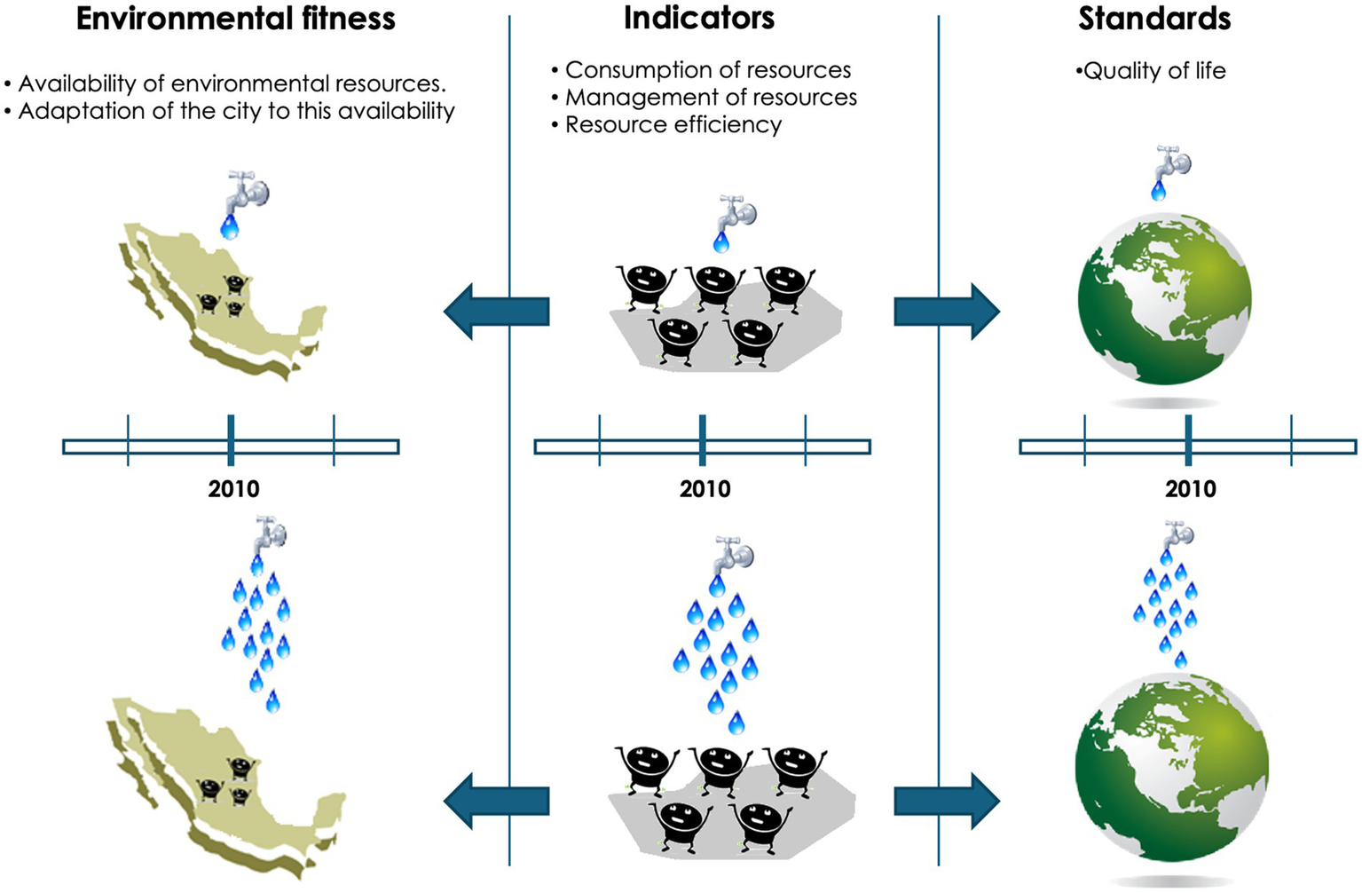
Relative sustainability of the city.
The matrices were developed by aggregating data on indicators from five-yearly time periods, thereby portraying the evolution of the cities under investigation from 1985 onwards. Furthermore, matrices with extreme values (maximum and minimum) of the same indicators in the same years were generated for Mexican capitals. These serve as comparison values for the study cities, providing insight into the relative performance of each (Figure 5).
Figure 5
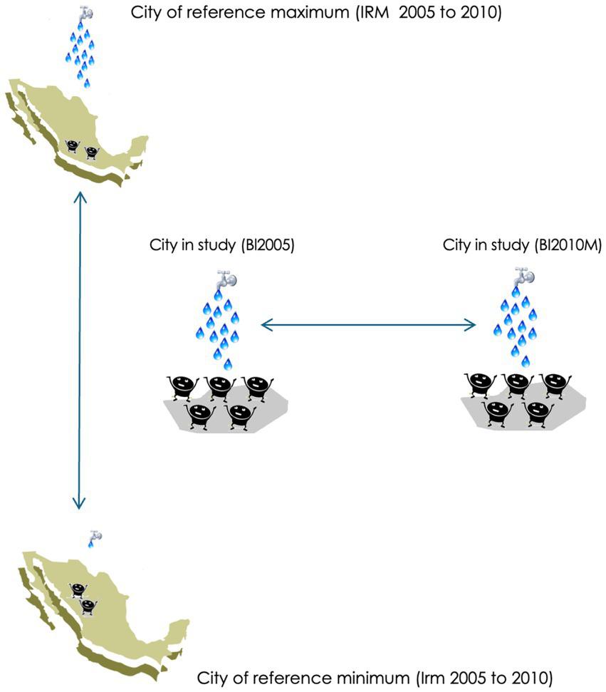
Aggregated efficiency scores.
The information obtained from comparing the reference indicators and the aggregated efficiency scores with the maximum and minimum values of the reference indicator ranges (Ir) per type of resource and for each subsystem (
Figure 6).
IRM = maximum reference indicator.
IRm = minimum reference indicator.
BIn = indicator for year n of the analyzed city.
Pefn = efficiency score.
Figure 6
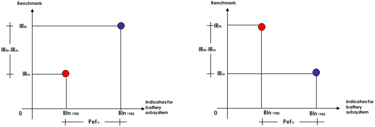
Positive and negative variation of an indicator vs. reference indicators.
The results of the comparison between the reference indicators and the efficiency scores with the maximum and minimum values were classified into the following categories:
Well above average: scores that are more than 1.5 times the standard deviation above the average.
Above average: scores that are between 0.5 and 1.5 times the standard deviation above the average.
Average: scores that are between 0.5 times the standard deviation below the mean and 0.5 times the standard deviation above the average.
Under the mean: scores falling between 0.5 and 1.5 times the standard deviation below the mean.
Well below the average: scores falling between 1.5 times the standard deviation below the mean.
2.3 Urban growth index
To ascertain the relationship between urban growth and the sustainability of this growth, an index (I
dus) is proposed for each indicator that states the relationships between the efficiency score (PEf
n) and the reference indicators (IR). The obtained values that tend to zero indicate greater sustainability. Conversely, the larger the number, the lower the sustainability.
Based on the values obtained from the time analysis per city, the following can be deduced:
If the values of the efficiency score are significantly disparate, it can be inferred that a process of change is occurring within the city. A positive value indicates investments and improvements in infrastructure, whereas a negative value signifies a decline in infrastructure. The disparity between these two values will be expressed in a numerical value that denotes the rate of growth. The larger this numerical value, the more rapid the growth will be.
If the efficiency scores differ only slightly, it indicates that the city is undergoing a relatively slow and gradual process of transformation. In contrast, if the scores differ significantly, this suggests a more rapid and pronounced change. A positive value signifies investments and improvements in infrastructure, while a negative value indicates a deterioration of the same. The magnitude of this difference will tend to be minimal, approaching zero.
In cases where the difference between the maximum and minimum reference values is minimal, this suggests that resource management or access may be a challenge in areas where growth has occurred during the period under consideration. Consequently, changes to infrastructure and efficiency are unlikely to have a significant impact on overall system efficiency. In such instances, the relationship between the maximum and minimum reference points tends to be approximately one.
If the maximum and minimum reference point values are significantly disparate, it can be inferred that the efficiency scores in the infrastructure systems exert a considerable influence on the overall city management. The relationship between the maximum and minimum reference points is typically found to be zero.
2.4 Characterization of sustainable urban growth patterns
The characterization of growth patterns can be achieved by determining the relationship between the three possible situations: (1) minimal changes in behavior with resources accessible; (2) minimal changes with resources inaccessible; and (3) high infrastructure changes (positive or negative). This will result in six possible results (
Figure 7).
Economizing growth refers to the scenario in which the urban structure remains largely unchanged in a favourable environment. This environment is characterized by accessible resources and the absence of external pressures, such as economic or population growth.
Weak growth: The urban structure remains essentially unaltered and is poorly adapted to the environment. In unfavorable environments with limited resources or significant external pressures—for example, those associated with economic growth or population increase.
Efficient growth: Cities adapted to the environmental context with investment in infrastructure. In a favorable environmental setting with accessible resources and without significant external pressures, such as economic and demographic growth.
Deficiency growth, not adapted to the environment: This refers to a scenario in which a decline of structures and urban infrastructure occurs as a result of a combination of deterioration and inadequate maintenance. This scenario occur in a favorable environmental context, with accessible resources, or in the absence of significant external pressures such as economic or demographic expansion.
Efficient growth and investment: Investments and high-structure and infrastructure changes. In an unfavorable environment, with inaccessible resources or with significant external pressures (economic or population growth).
Deficient growth and degradation: Changes in the condition of the structure and urban infrastructure resulting from a lack of maintenance and degradation. In an environment that is unfavorable for growth, with inaccessible resources, or with significant external pressures (economic or population growth).
Figure 7
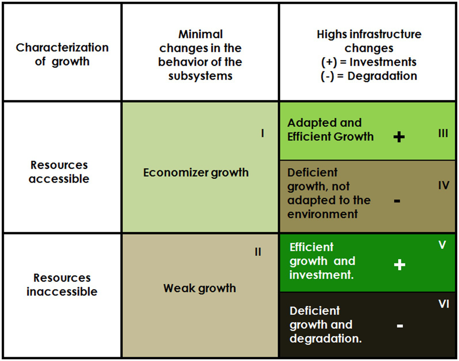
Growth characterization.
2.5 Evaluation of the sustainable development
Once the efficiency score values for each resource have been calculated, these values are applied to the indicators to obtain a qualitative and descriptive classification of the urban growth pattern in terms of sustainability. While this characterization allows for a relative classification of growth, it does not determine its sustainability. However, when used in conjunction with the matrix of indicators by time periods - which describes the city’s growth in two, three and four dimensions - it allows us to define whether it is a scenario close to or far from of fitness, based on both resource management and adaptation to the environment.
It can be described as the maintenance of the oldest urban areas in a state of good repair, the development of intermediate urban areas in an economically efficient and appropriate manner, and minimal growth in new urban areas while conserving material and energy resources. Conversely, an unsustainable city does not maintain adequate conditions in its oldest urban areas, lacks adequate development, and fails to adapt to its intermediate urban areas. Additionally, it wastes resources on new areas of urban development with expansion and periphery (Figure 8).
Figure 8
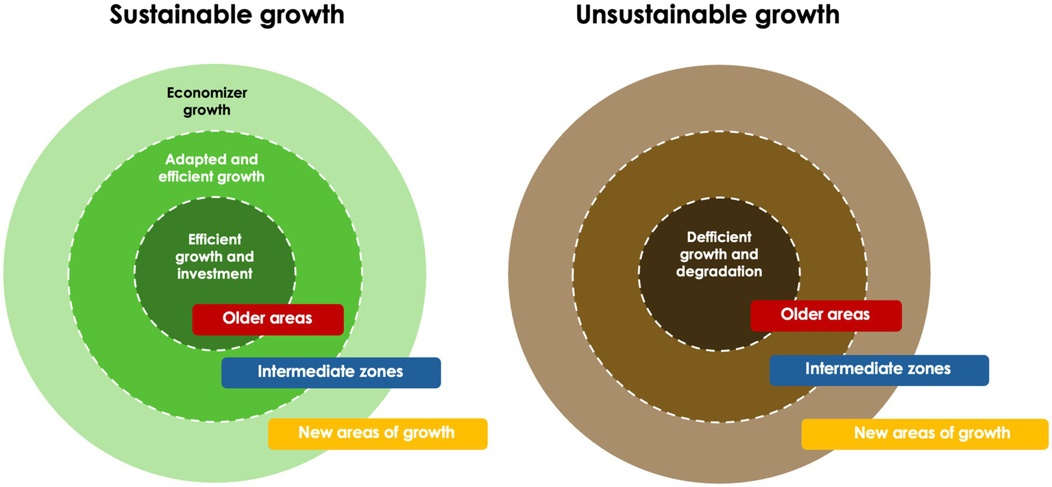
Sustainable and unsustainable growth.
The combination of the six growth patterns (66) results in a total of 4,665,600 potential combinations. From these, we can identify a combination that could come close to the definition of resilient urban growth, which encompasses the maintenance of urban infrastructure, policies, and systems that can withstand adverse shocks, minimize the vulnerability of people and communities, and facilitate rapid recovery from disruptive events. And on the contrary, fragile or non-resilient urban growth, with urban areas that are unprepared to face the challenges and disturbances that may arise, with inadequate infrastructure, a lack of urban planning, vulnerability to adverse events, dependence on a single economic sector, lack of community participation, and a lack of adaptation to the environment with high urban sprawl and peripheral growth in an environment with few resources (Figure 9).
Figure 9
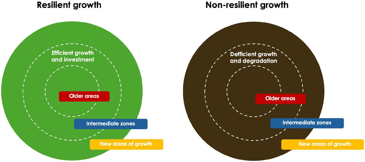
Resilient and non-resilient growth.
A comparative study of the growth of three Mexican cities can be used to illustrate and analyze the characteristics of urban growth in two, three, and four dimensions.
3 City selection
In Mexico, the Valley of Mexico, or central region of the country, is the most densely populated in Mexico, with an estimated population of 21 million inhabitants in 2020, according to the National Institute of Statistics and Geography (INEGI), and it concentrates a higher level of economic activity, infrastructure, and services than any other metropolitan area in the country. This is related to the regional integration of cities in a network that connects different states and municipalities functionally, spatially, and in terms of connectivity. Some cities in this region are in a conurbation—physical continuity—and, in some cases, form metropolitan areas by occupying more than one administrative and political unit. Metropolitan areas and contiguous cities form a metropolitan zone, which is formed by all adjacent full municipalities in which they are located. The cities included in this study were selected based on their proximity and relationship to the expansion of Mexico City, their growth history and projections, and the similarity and comparability of their socioeconomic profiles. Toluca, Cuernavaca, and Pachuca are the three cities closest to Mexico City (Figure 10). They are located along its urban development axis and are therefore likely to become part of its metropolitan area; they are all state capitals, comparable in their characteristics and similar in their functional relationships with Mexico City, receiving large amounts of waste generated there and providing it with environmental services.
Figure 10
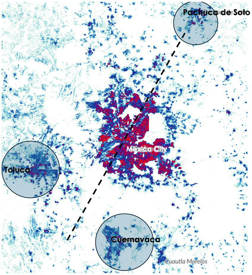
Recuperated and modified by “World Population Density” (https://luminocity3d.org/WorldPopDen/#10/22.2656/-97.8058).
Mexico City is forcing major changes on the surrounding rural and urban centers, generating growth and development in the region. The land around small towns is transformed as it is taken over by industries located outside the city. The natural environment of the region’s sparsely populated areas becomes housing and recreational space for an increasing number of urban dwellers, and traditional land uses change without control or adequate planning. The growth of Mexico City indirectly promotes the urbanization of these areas that have provided environmental services to Mexico City. The municipalities of Cuernavaca, Toluca, and Pachuca are located outside the Mexico City metropolitan area, have a predominantly urban character, and maintain a strong level of functional relationships with Mexico City, such as having a significant number of residents who commute to their jobs in the central municipalities of the Mexico City metropolitan area. The cities analyzed in this study are considered metropolitan areas, a term that in this case means the set of two or more municipalities in which there is a city of more than 50,000 inhabitants with an urban area, functions, and activities that extend beyond the limits of the municipality in which the city was originally located, and that includes predominantly urban neighboring municipalities or has a direct influence on them, as well as a high degree of socioeconomic integration with them. Over the last 30 years, urban sprawl has created a discontinuous, dispersed, and low-density model for Mexican cities. The objective of the identification and delineation of metropolitan zones is to create a common and comparable statistical geography.
4 Results
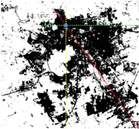
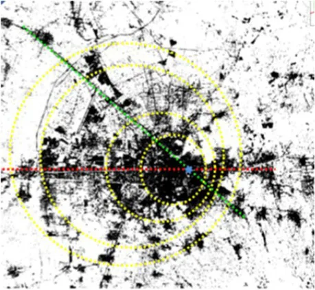
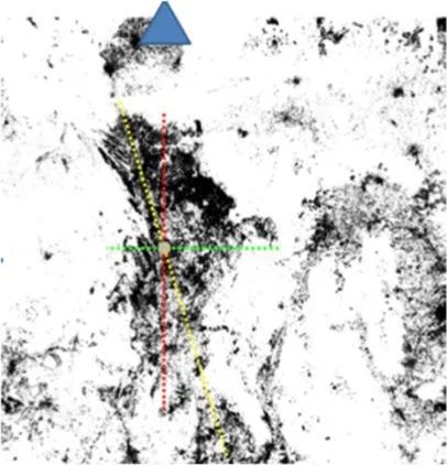
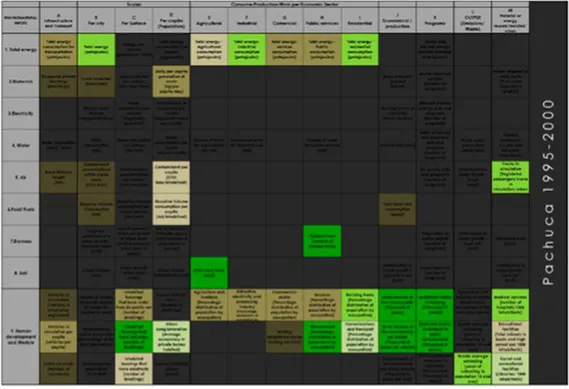
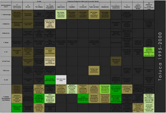
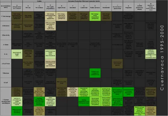
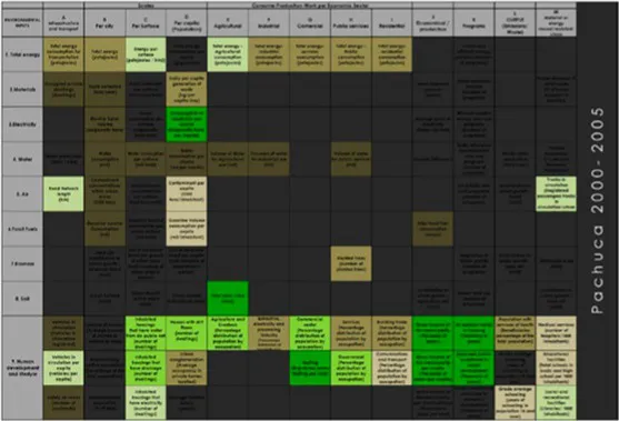
Tables 7, 8 show the results of the application of the methodology in the form of a diagram. Historical–geographical, per subsystem, per type or resource, per type of inputs and outputs (or growth pattern), from 1995 to 2000 in periods of 5 years (Figure 11).
Figure 11

Sustainable growth patterns—Cuernavaca/Toluca/Pachuca.
Table 7
| Sustainable urban growth patterns based on environmental fitness | |||
|---|---|---|---|
| Pachuca | Toluca | Cuernavaca | |
| The orientation of Pachuca’s growth is to the Southwest (to Mexico City), South, and West. It does not grow to the north and northeast in the mountains. | The orientation of Toluca’s growth is both to the East and Northeast (to Mexico City). | Cuernavaca’s growth to the East and South, where there were rain-fed and irrigation fields or secondary vegetation. In the other orientations, it does not grow due to the mountains and topography. | |
| Two dimensions |
|
|
|
| Three dimensions | |||
|
|
|
|
| Fourth dimensions |
|
|
|
|
|

|
|
Growth axis of Cuernavaca, Toluca, and Pachuca.
Table 8
| Period | City | Deficient growth and degradation (%) | Deficient growth, not adapted to the environment | Weak growth | (−) | Efficient growth and investment (%) | Adapted and efficient growth | Economizer growth | (+) | Total |
|---|---|---|---|---|---|---|---|---|---|---|
| 1994–2000 | Cuernavaca | 34 | 7.3 | 12 | −128.6 | 17.07 | 17 | 12 | 97.21 | −31.39 |
| Toluca | 29.2 | 31.7 | 4.8 | −155.8 | 14.6 | 4.8 | 12 | 65.4 | −90.4 | |
| Pachuca | 21.9 | 24.3 | 12.19 | −126.49 | 19.5 | 17.07 | 7.3 | 99.04 | −26.55 | |
| 2000–2005 | Cuernavaca | 43 | 26 | 9.7 | −190.7 | 9.7 | 14.6 | 17 | 75.3 | −155.4 |
| Toluca | 41.4 | 6 | 4.8 | −141 | 21.9 | 24.3 | 19.5 | 133.8 | −7.2 | |
| Pachuca | 34.14 | 31.7 | 14.6 | −180.42 | 17.07 | 14.6 | 17.07 | 97.48 | −82.94 | |
| 2005–2010 | Cuernavaca | 39 | 9.7 | 7.3 | −143.7 | 31.7 | 39 | 17 | 190.1 | 46.4 |
| Toluca | 48.7 | 14.6 | 14.6 | −189.9 | 31.7 | 12.19 | 12.19 | 131.67 | −58.23 | |
| Pachuca | 51.2 | 12.19 | 12.19 | −190.17 | 26.8 | 17.07 | 14.6 | 129.14 | −61.03 |
Summary table—growth patterns.
5 Discussion of results
The results show large variations between the patterns of growth and sustainability characteristics of these types of growth, both by resource type for the efficient use of resources and in the Calidad of life and periods. Overall, growth rates do not reflect a development oriented toward sustainability. The growth factors respond to human needs and resource availability. Programs, plans, and strategies for urban sustainability have not yet been reflected in reality. Any effort directed to this effect shall seek equity, livability, and viability for the city. And the feasibility, necessity, and effectiveness of these strategies should be evaluated.
For the city of Toluca, in the period 1995–2000, the city presents 13 indicators of Deficient Growth and Degradation, 3 indicators of Deficient Growth Not Adapted to the Environment, and 2 indicators of Weak Growth. This makes a total of 22 indicators (43%) of unsustainable growth. Moreover, it features six growth indicators for efficient investment. For 2000–2005, the city rose to 17 indicators of Deficient Growth and Degradation, 5 indicators of Deficient Growth Not Adapted to the Environment, and 1 indicator of Weak Growth, which makes a total of 23 indicators (56%) of unsustainable growth. On the other hand, the number of efficient growth indicators increased to 7. This involves partial improvement in some ways, but we can say that growth remains similar to the previous period. For the period 2005–2010, the city presents 20 indicators of Deficient Growth and Degradation, 6 indicators of Deficient Growth Not Adapted to the Environment, and 4 indicators of Weak Growth, which makes a total of 30 indicators (73%) of no growth sustainable. It also presents the positive side: 12 indicators of efficient growth and investment. This city is noted for growth that has remained unsustainable for three periods.
In general terms, it is identified that the growth sustainability patterns of the cities of Pachuca and Toluca present weak growth; the urban structure remains essentially unaltered and is poorly adapted to the environment. In unfavorable environments with limited resources or significant external pressures. While Cuernavaca goes from weak to deficient growth not adapted to the environment with a decline in the condition of structures and urban infrastructure resulting from a combination of deterioration and inadequate maintenance in a favorable environmental context, to finally, toward an economizing growth in which urban structure remains largely unchanged in a favorable environment.
6 Reflections on the approach and limitations of the study
The main limitation of the analysis is the need for local indicators to be periodically updated to perform a long-term study. The construction of a generic urban environmental fitness matrix can be adapted to the availability of information for the construction of indicators that can provide temporal continuity. In Mexico, the availability and consistency of data are limited. This research uses indicators from different administrative levels. Since indicators are scaled by the corresponding area, population, or GDP, their use should not significantly decrease the degree to which they are comparable. Therefore, metropolitan areas can have noticeable variations from one city to another. To try and overcome data gaps, strong theoretical techniques should be considered when calculating estimates. Moreover, the potential effects of factors such as “access to water” or “access to sanitation.” should also be considered. While informal settlements vary in size and definition, they generally lack data on infrastructure, access to public services, and population. Due to this, it is necessary to use digital maps to analyze real references that are not formally registered. The indicator collection in this study also includes those that are commonly used as references, which include reviews from the National Institute of Geography and Informatics and the Secretariat of Environment.
Current indicators provide valuable information about the material and energy balance in various areas. This information is available and generated by local governments, and it plays a crucial role in designing policies and programs related to energy efficiency, the use of resources, and human welfare. The information available in Mexico helps researchers to collect data on total energy, water, electricity, and general human welfare. Regarding the level of analysis, the current local information allows researchers to ascertain the performance on the three scales of analysis—city, surface, and per capita—as well as the level of outputs and recycling of energy and matter. The proposed indicators are mostly related to the geographic information system that was generated to measure changes in local land use and are related to the dimensions of soil and biomass. Similarly, the other group of proposed indicators is related to the analysis of programs aimed at material, energy, and clean efficiency in government sectors, and they indicate a better environmental performance of cities at the local level, as well as the increasing level of clean, recycled, or reused materials and energy. In the case of indicators taken from other sources, it is important to note that these indicators already exist and are measured in other countries or at scales different from the local ones. Similarly, it is important to generate information that does not exist in Mexico to ensure that we have indicators that provide a complete knowledge of the uses and applications of the material and energy balance of a city.
Productive activities use environmental resources, thus transforming them into goods and services with market values to obtain benefits and externalize costs to society. The resources and services provided by the environment, such as intermediate inputs, such as capital, energy, and human labor, transform into goods on the one hand and into damages to society on the other, thus generating residual emissions with different degrading properties and toxicity to the environment and human health. The statistics on how natural resources and environmental services are transformed through human activities into goods and necessities for society can be handy warning indicators of environmental change and the misuse of raw materials as well as resources provided by natural ecosystems. The interrelation of productive processes with natural and environmental resources, as well as their socioeconomic importance, are related to environmental impacts and degradation, risks, and the running down of natural resources: agriculture and livestock, manufacturing industry, transport, energy, tourism, and residues. There are statistics regarding cities’ tendencies toward the management and disposal of solid municipal residue and representative data as to the production and installed capacity for treating and confining dangerous industrial residues, as well as a reference to the characteristics of the rubbish produced in cities, which include homemade rubbish and that coming from other sources (commercial, institutional, construction, demolition, etc.).
As an alternative, it is identified to use as benchmark world indicators such as the Human Development Index (HDI), which measures human development based on indicators such as life expectancy at birth, access to education, and per capita income level; the Ecological Footprint; the Environmental Sustainability Index (ESI); the Sustainable Development Index (SDI); sustainable building certifications or urban sustainability indicators from organizations such as the World Bank, the Organization for Economic Cooperation and Development (OECD), and the United Nations Human Settlements Programme (UN-Habitat).
7 Conclusion
Fitness underpins some theories of urban sustainability that try to transform the city from an open to a closed and environmentally adapted system during its design, operation, and/or regeneration. Transforming an open system into a closed system involves introducing elements of control and feedback to make the system self-regulating.
Environmental fitness is proposed as a systemic approach of sustainability urban growth patterns that explores ways to develop closed-loop urban systems with multiple indicators organized by subsystems and in two, three, and four dimensions.
Some applications of the urban environmental fitness matrix are: in planning and design, the restoration of ecological systems and degraded lands will require the design of standards and implementation of best practice requirements to anticipate problems and improve the benefits of environmental regulation efforts, from legal obligations and prohibitions directed at a variety of public and private actors as well as obligations; in new urban business models, innovative business models for companies that hold a significant part of the market and that have the capacity to activate the horizontal phases of the vectors and expand geographically. In the design of public policies for urban reverse cycles, the use of materials in several cycles and the final return of the materials to the soil or to the industrial production system means the logistics of the supply chain, selection, storage, risk management, or energy generation, with optimal collection and lower costs in systems of treatment.
The six sustainable urban growth patterns that emerged have potential for describing urban growth sustainability patterns and have significant practical applications in urban planning, urban renovation, strategies of urban circularity, sustainable development management, and mitigation of urban sprawl. These patterns can also aid in understanding the dynamics of urbanization, simulating population decentralization, modeling informal urbanization, and predicting urban growth by integrating socioeconomic factors.
Urban growth presents both challenges and opportunities for cities in terms of providing urban land, reducing environmental impacts, and improving the efficiency of infrastructure networks.
Statements
Data availability statement
The raw data supporting the conclusions of this article will be made available by the authors, without undue reservation.
Author contributions
MU-M: Conceptualization, Methodology, Writing – original draft, Writing – review & editing.
Funding
The author(s) declare that financial support was received for the research, authorship, and/or publication of this article. The present study is framed under postdoctoral studies at Tecnológico de Monterrey and was supported by the Inter-American Development Bank (Key: RGT 2 6 6 3).
Conflict of interest
The author declares that the research was conducted in the absence of any commercial or financial relationships that could be construed as a potential conflict of interest.
Publisher’s note
All claims expressed in this article are solely those of the authors and do not necessarily represent those of their affiliated organizations, or those of the publisher, the editors and the reviewers. Any product that may be evaluated in this article, or claim that may be made by its manufacturer, is not guaranteed or endorsed by the publisher.
References
1
Aguilera F. Valenzuela L. Botequilha-Leitão A. (2011). Landscape metrics in the analysis of urban land use patterns: a case study in a Spanish metropolitan area. Landsc. Urban Plan.99, 226–238. doi: 10.1016/J.LANDURBPLAN.2010.10.004
2
Aithal B. Ramachandra T. (2016). Visualization of urban growth pattern in Chennai using Geoinformatics and spatial metrics. J Indian Soc Remote Sens44, 617–633. doi: 10.1007/s12524-015-0482-0
3
Bagan H. Yamagata Y. (2012). Landsat analysis of urban growth: how Tokyo became the world's largest megacity during the last 40 years. Remote Sens. Environ.127, 210–222. doi: 10.1016/J.RSE.2012.09.011
4
Batty M. Marshall S. (2009). The evolution of cities: Geddes, Abercrombie and the new physicalism. Town Plan. Rev.80, 551–574. doi: 10.3828/TPR.2009.12
5
Ben-Eli M. U. (2018). Sustainability: definition and five core principles, a systems perspective. Sustain. Sci.13, 1337–1343. doi: 10.1007/s11625-018-0564-3
6
Bryant M. M. Turner J. S. (2019). From thermodynamics to creativity: McHarg’s ecological planning theory and its implications for resilience planning and adaptive design. Soc Ecol Pract Res1:271. doi: 10.1007/s42532-019-00027-1
7
Des Roches S. Brans K. I. Lambert M. R. Rivkin L. R. Savage A. M. Schell C. J. et al . (2021). Socio-eco-evolutionary dynamics in cities. Evolution Appl14:65. doi: 10.1111/eva.13065
8
Fenta A. Yasuda H. Haregeweyn N. Belay A. Hadush Z. Gebremedhin M. et al . (2017). The dynamics of urban expansion and land use/land cover changes using remote sensing and spatial metrics: the case of Mekelle City of northern Ethiopia. Int. J. Remote Sens.38, 4107–4129. doi: 10.1080/01431161.2017.1317936
9
Li C. Duan X. (2020). Exploration of urban interaction features based on the cyber information flow of migrant concern: A case study of China’s main urban agglomerations. Int. J. Environ. Res. Public Health17:235. doi: 10.3390/ijerph17124235
10
Mahtta R. Mahendra A. Seto K. (2019). Building up or spreading out? Typologies of urban growth across 478 cities of 1 million+. Environ. Res. Lett.14:ab59bf. doi: 10.1088/1748-9326/ab59bf
11
Moore D. Hague D. J. (2019). Introduction to systems thinking. Building Production Management Techniques. Taylor & Francis Group, 1–12.
12
Mou Y. Song Y. Xu Q. He Q. Hu A. (2018). Influence of urban-growth pattern on air quality in China: a study of 338 cities. Int. J. Environ. Res. Public Health15:1805. doi: 10.3390/ijerph15091805
13
Opromolla A. Volpi V. (2020). Cities as Complex Systems. Int J Urban Plan Smart Cities1:101. doi: 10.4018/ijupsc.2020070101
14
Qian Y. Chen Y. Lin C. Wang W. Zhou W. (2019). Revealing patterns of greenspace in urban areas resulting from three urban growth types. Phys Chem Earth110, 14–20. doi: 10.1016/J.PCE.2019.02.013
15
Schipper L. Meyers S. (1992). Energy efficiency and human activity: past trends, future prospects. Cambridge: Cambridge University Press.
16
Shi Y. Sun X. Zhu X. Li Y. Mei L. (2012). Characterizing growth types and analyzing growth density distribution in response to urban growth patterns in peri-urban areas of Lianyungang City. Landsc. Urban Plan.105, 425–433. doi: 10.1016/J.LANDURBPLAN.2012.01.017
17
Subasinghe S. (2019). Urban growth: from pixel to reality. Abstracts ICA.1:2019. doi: 10.5194/ICA-ABS-1-353-2019
18
The University of Chicago Press (2016). “The fitness of the environment, an inquiry into the biological significance of the properties of matter” in The American naturalist. ed. HendersonL. J., vol. 47 (The Harvard Universit), 105–115.
19
Yang B. Li S. (2019). Blending project goals and performance goals in ecological planning: Ian McHarg’s contributions to landscape performance evaluation. Soc Ecol Pract Res1, 209–225. doi: 10.1007/s42532-019-00029-z
20
Živković J. (2020). Urban Form and Function. In: Climate Action. Encyclopedia of the UN Sustainable Development Goals. eds. Leal FilhoW.AzulA. M.BrandliL.ÖzuyarP. G.WallT. (Cham: Springer).
Summary
Keywords
urban sustainability, environmental fitness, urban growth, sustainable urban growth patterns, indicators of sustainability
Citation
Ugalde-Monzalvo M (2024) Sustainable urban growth patterns based on environmental fitness. Front. Sustain. Cities 6:1382180. doi: 10.3389/frsc.2024.1382180
Received
05 February 2024
Accepted
24 June 2024
Published
26 July 2024
Volume
6 - 2024
Edited by
Sudhir Chella Rajan, Indian Institute of Technology Madras, India
Reviewed by
Pablo Torres-Lima, Metropolitan Autonomous University, Mexico
Paunita Iuliana Boanca, University of Agricultural Sciences and Veterinary Medicine of Cluj-Napoca, Romania
Updates
Copyright
© 2024 Ugalde-Monzalvo.
This is an open-access article distributed under the terms of the Creative Commons Attribution License (CC BY). The use, distribution or reproduction in other forums is permitted, provided the original author(s) and the copyright owner(s) are credited and that the original publication in this journal is cited, in accordance with accepted academic practice. No use, distribution or reproduction is permitted which does not comply with these terms.
*Correspondence: Marisol Ugalde-Monzalvo, marisol.ugalde@tec.mx
Disclaimer
All claims expressed in this article are solely those of the authors and do not necessarily represent those of their affiliated organizations, or those of the publisher, the editors and the reviewers. Any product that may be evaluated in this article or claim that may be made by its manufacturer is not guaranteed or endorsed by the publisher.