Regularized Kernel Algorithms for Support Estimation

1. Introduction

A classical issue in statistics is support estimation, i.e., the problem of learning the support of a probability distribution from a set of points identically sampled according to the distribution. For example, the Devroye-Wise algorithm [1] estimates the support with the union of suitable balls centered in the training points. In the last two decades, many algorithms have been proposed and their statistical properties analyzed [1–14] and references therein.

An instance of the above setting, which plays an important role in applications, is the problem of novelty/anomaly detection, see Campos et al. [15] for an updated review. In this context, in Hoffmann [16] the author proposed an estimator based on Kernel Principal Component Analysis (KPCA), first introduced in Schölkopf et al. [17] in the context of dimensionality reduction. The algorithm was successfully tested in many applications from computer vision to biochemistry [18–24]. In many of these examples the data are often represented by high dimensional vectors, but they actually live close to a nonlinear low dimensional submanifold of the original space, and the proposed estimator takes advantage of the fact that KPCA provides an efficient compression/dimensionality reduction of the original data [16, 17], whereas many classical set estimators refer to the dimension of the original space, as it happens for the Devroye-Wise algorithm.

In this paper we prove that KPCA is a consistent estimator of the support of the distribution with respect to the Hausdorff distance. The result is based on an intriguing property of the reproducing kernel, called separating condition, first introduced in De Vito et al. [25]. This assumption ensures that any closed subset of the original space is represented in the feature space by a linear subspace. We show that this property remains true if the data are recentered to have zero mean in the feature space. Together with the results in De Vito et al. [25], we conclude that the consistency of KPCA algorithm is preserved by recentering of the data, which can be regarded as a degree of freedom to improve the empirical performance of the algorithm in a specific application.

Our main contribution is sketched in the next subsection together with some basic properties of KPCA and some relevant previous works. In section 2, we describe the mathematical framework and the related notations. Section 3 introduces the spectral support estimator and informally discusses its main features, whereas its statistical properties and the meaning of the separating condition for the kernel are analyzed in section 4. Finally section 5 presents the effective algorithm to compute the decision function and discusses the role of the two meta-parameters based on the previous theoretical analysis. In the Appendix (Supplementary Material), we collect some technical results.

1.1. Sketch of the Main Result and Previous Works

In this section we sketch our main result by first recalling the construction of the KPCA estimator introduced in Hoffmann [16]. We have at disposal a training set $\left\{x_1,\dots ,x_n\right\}\in {D}\subset {ℝ}^d$ of n points independently sampled according to some probability distribution P. The input space ${D}$ is a known compact subset of ℝ^d, but the probability distribution P is unknown and the goal is to estimate the support C of P from the empirical data. We recall that C is the smallest closed subset of ${D}$ such that ℙ[C] = 1 and we stress that C is in general a proper subset of ${D}$, possibly of low dimension.

Classical Principal Component Analysis (PCA) is based on the construction of the vector space V spanned by the first m eigenvectors associated with the largest eigenvalues of the empirical covariance matrix

$\frac{1}{n}{\displaystyle \sum _{i=1}^n(x_i-\overline{x})}\otimes (x_i-\overline{x}),$

where $\overline{x}=\frac{1}{n}\sum _{i=1}^n{x}_i$ is the empirical mean. However, if the data do not live on an affine subspace, the set V is not a consistent estimator of the support. In order to take into account non-linear models, following the idea introduced in Schölkopf et al. [17] we consider a feature map Φ from the input space ${D}$ into the corresponding feature space ${H}$, which is assumed to be a Hilbert space, and we replace the empirical covariance matrix with the empirical covariance operator

$\widehat{T_n^c}=\frac{1}{n}{\displaystyle \sum _{i=1}^n(\Phi (}{x}_i)-{\widehat{\mu }}_n)\otimes (\Phi (x_i)-{\widehat{\mu }}_n),$

where ${\hat{\mu }}_n=\frac{1}{n}\sum _{i=1}^n\Phi (x_i)$ is the empirical mean in the feature space. As it happens in PCA, we consider the subspace ${\hat{V}}_{m,n}$ of ${H}$ spanned by the first m- eigenvectors ${\widehat{f}}_1,\dots ,{\widehat{f}}_m$ of $\widehat{T_n^c}$. According to the proposal in Hoffmann [16], we consider the following estimator of the support of the probability distribution P

${\widehat{C}}_n=\left\{x\in {D}\mid \Vert {\widehat{\mu }}_n+{\displaystyle \sum _{j=1}^m\langle \Phi (x)-{\widehat{\mu }}_n,{\widehat{f}}_j\rangle {\widehat{f}}_j-\Phi (x)}\Vert \le {\tau }_n\right\},$

where τ_n is a suitable threshold depending on the number of examples and

${\widehat{\mu }}_n+{\displaystyle \sum _{j=1}^m\langle \Phi (x)-{\widehat{\mu }}_n,{\widehat{f}}_j\rangle }{\widehat{f}}_j$

is the projection of an arbitrary point $x\in {D}$ onto the affine subspace ${\hat{\mu }}_n+{\hat{V}}_{m,n}$. We show that, under a suitable assumption on the feature map, called separating property, ${\hat{C}}_n$ is a consistent estimator of C with respect to the Hausdorff distance between compact sets, see Theorem 3 of section 4.2.

The separating property was introduced in De Vito et al. [25] and it ensures that the feature space is rich enough to learn any closed subset of ${D}$. This assumption plays the same role of the notion of universal kernel [26] in supervised learning.

Moreover, following [25, 27] we extend the KPCA estimator to a class of learning algorithms defined in terms of a low-pass filter function r_m(σ) acting on the spectrum of the covariance matrix and depending on a regularization parameter m ∈ ℕ. The projection of ${\hat{\Phi }}_n(x)$ onto ${\hat{V}}_{m,n}$ is replaced by the vector

${\widehat{\Phi }}_{n,m}(x)={\displaystyle \sum _{j=1}^{+\infty }{r}_m}({\widehat{\sigma }}_j)\langle \Phi (x)-{\widehat{\mu }}_n,{\widehat{f}}_j\rangle {\widehat{f}}_j,$

where ${\left\{{\widehat{f}}_j\right\}}_j$ is the family of eigenvectors of $\widehat{T_n^c}$ and ${\left\{{\widehat{\sigma }}_j\right\}}_j$ is the corresponding family of eigenvalues. The support is then estimated by the set

$\{x\in {D}\mid ||{\widehat{\mu }}_n+{\widehat{\Phi }}_{n,m}(x)-\Phi (x)||\le {\tau }_n\}.$

Note that KPCA corresponds to the choice of the hard-cut off filter

$r_m({\widehat{\sigma }}_j)=\{\begin{array}{ll}1\hfill & i\le m\hfill \\ 0\hfill & i>m\hfill \end{array}.$

However, other filter functions can be considered, inspired by the theory of regularization for inverse problems [28] and by supervised learning algorithms [29, 30]. In this paper we show that the explicit computation of these spectral estimators reduces to a finite dimensional problem depending only on the kernel K(x, w) = 〈Φ(x), Φ(w)〉 associated with the feature map, as for KPCA. The computational properties of each learning algorithm depend on the choice of the low-pass filter r_m(σ), which can be tuned to out-perform of some specific data set, see the discussion in Rudi et al. [31].

We conclude this section with two considerations. First, in De Vito et al. [25, 27] it is proven a consistency result for a similar estimator, where the subspace ${\hat{V}}_{n,m}$ is computed with respect to the non-centered covariance matrix in the feature space ${H}$, instead of the covariance matrix. In this paper we analyze the impact of recentering the data in the feature space ${H}$ on the support estimation problem, see Theorem 1 below. This point of view is further analyzed in Rudi et al. [32, 33].

Finally note that, our consistency results are based on convergence rates of empirical subspaces to true subspaces of the covariance operator, see Theorem 2 below. The main difference between our result and the result in Blanchard et al. [34], is that we prove the consistency for the case when the dimension m = m_n of the subspace ${\hat{V}}_{m,n}$ goes to infinity slowly enough. On the contrary, in their seminal paper [34] the authors analyze the most specific case when the dimension of the projection space is fixed.

2. Mathematical Assumptions

In this section we introduce the statistical model generating the data, the notion of separating feature map and the properties of the filter function. Furthermore, we show that KPCA can be seen as a filter function and we recall the main properties of the covariance operators.

We assume that the input space ${D}$ is a bounded closed subset of ℝ^d. However, our results also hold true by replacing ${D}$ with any compact metric space. We denote by d(x, w) the Euclidean distance |x − w| between two points x, w ∈ ℝ^d and by d_H(A, B) the Hausdorff distance between two compact subsets $A,B\subset {D}$, explicitly given by

$d_{{}_H}(A,B)=\max \left\{\underset{x\in A}{\sup }\text{d}(x,B),\underset{x\in B}{\sup }\text{d}(x,A)\right\},$

where $\mathrm{\text{d}}(x,A)={inf}_{w\in A}\mathrm{\text{d}}(x,w)$.

2.1. Statistical Model

The statistical model is described by a random vector X taking value in ${D}$. We denote by P the probability distribution of X, defined on the Borel σ-algebra of ${D}$, and by C the support of P.

Since the probability distribution P is unknown, so is its support. We aim to estimate C from a training set of empirical data, which are described by a family X₁, …, X_n of random vectors, which are independent and identically distributed as X. More precisely, we are looking for a closed subset ${\hat{C}}_n={\hat{C}}_{X_1,\dots ,X_n}\subset {D}$, depending only on X₁, …, X_n, but independent of P, such that

$\mathbb{P}\left[\underset{n\to +\infty }{\lim }{d}_{{}_H}({\widehat{C}}_n,C)=0\right]=1$

for all probability distributions P. In the context of regression estimate, the above convergence is usually called universal strong consistency [35].

2.2. Mercer Feature Maps and Separating Condition

To define the estimator ${\hat{C}}_n$ we first map the data into a suitable feature space, so that the support C is represented by a linear subspace.

Assumption 1. Given a Hilbert space ${H}$, take $\Phi :{D}\to {H}$ satisfying the following properties:

(H1) the set $\Phi ({D})$ is total in ${H}$, i.e.,

$\overline{\text{span}}\{\widehat{\Phi }(x)\mid x\in {D}\}={H},$

where $\overline{\mathrm{\text{span}}}\left\{·\right\}$ denotes the closure of the linear span;

(H2) the map Φ is continuous.

The space ${H}$ is called the feature space and the map Φ is called a Mercer feature map.

In the following the norm and scalar product of ${H}$ are denoted by ||·|| and 〈··〉, respectively.

Assumptions (H1) and (H2) are standard for kernel methods, see Steinwart and Christmann [36]. We now briefly recall some basic consequences. First of all, the map $K:{D}\times {D}\to ℝ$

$K(x,w)=\langle \Phi (x)\Phi (w)\rangle$

is a Mercer kernel and we denote by ${{H}}_K$ the corresponding (separable) reproducing kernel Hilbert space, whose elements are continuous functions on ${D}$. Moreover, each element $f\in {H}$ defines a function $f_{\Phi }\in {{H}}_K$ by setting f_Φ(x) = 〈f, Φ(x)〉 for all $x\in {D}$. Since $\Phi ({D})$ is total in ${H}$, the linear map f ↦ f_Φ is an isometry from ${H}$ onto ${{H}}_K$. In the following, with slight abuse of notation, we write f instead of f_Φ, so that the elements $f\in {H}$ are viewed as functions on ${D}$ satisfying the reproducing property

$f(x)=\langle f,\Phi (x)\rangle x\in {D}.$

Finally, since ${D}$ is compact and Φ is continuous, it holds that

$\begin{array}{cc}R=\underset{x\in {D}}{\sup }\left|\right|\Phi (x)|{|}^2=\underset{x\in {D}}{\sup }K(x,x)<+\infty .& \left(1\right)\end{array}$

Following De Vito et al. [27], we call Φ a separating Mercer feature map if the following the separating property also holds true.

(H3) The map Φ is injective and for all closed subsets ${C}\subset {D}$

$\begin{array}{cc}\Phi ({C})=\Phi ({D})\cap \overline{\text{span}}\{\Phi (x)\mid x\in {C}\}.& \left(2\right)\end{array}$

It states that any closed subset ${C}\subset {D}$ is mapped by Φ onto the intersection of $\Phi ({D})$ and the closed subspace $\overline{\mathrm{\text{span}}}\left\{\Phi (x)\mid x\in {C}\right\}\subset {H}$. Examples of kernels satisfying the separating property are for ${D}\subset {ℝ}^d$ [27]:

• Sobolev kernels with smoothness index $s>\frac{d}{2}$;

• the Abel/Laplacian kernel K(x, w) = e ^{− γ|x − w|} with γ > 0;

• the ℓ₁-kernel $K(x,w)=e^{-\gamma |x-w{|}_1}$, where |·|₁ is the ℓ₁-norm and γ > 0.

As shown in De Vito et al. [25], given a closed set ${C}$ the equality (2) is equivalent to the condition that for every $x_0\notin {C}$ there exists $f\in {H}$ such that

$\begin{array}{cc}f(x_0)\ne 0\text{and}f(x)=0\forall x\in {C}.& \left(3\right)\end{array}$

Clearly, an arbitrary Mercer feature map is not able to separate all the closed subsets, but only few of them. To better describe these sets, we introduce the elementary learnable sets, namely

${{C}}_f=\{x\in {D}\mid f(x)=\langle f,\Phi (x)\rangle =0\},$

where $f\in {H}$. Clearly, ${{C}}_f$ is closed and the equality (3) holds true. Furthermore the intersection of an arbitrary family of elementary learnable sets ${\cap }_{f\in {F}}{C}_f$ with ${F}\subset {H}$ satisfies (3), too. Conversely, if ${C}$ is a set satisfying (2), select a maximal family {f_j}_j∈J of orthonormal functions in ${H}$ such that

$f_j(x)=\langle f_j,\Phi (x)\rangle =0\forall x\in {C},j\in J,$

i.e., a basis of the orthogonal complement of $\left\{\Phi (x)\mid x\in {C}\right\}$, then it is easy to prove that

$\begin{array}{cc}{C}=\{x\in {D}\mid f_j,\Phi (x)\rangle =0\forall j\in J\}={\displaystyle \underset{j\in J}{\cap }{C}_{f_j}},& \left(4\right)\end{array}$

so that any set which is separating by Φ is the (possibly denumerable) intersection of elementary sets. Assumption (H3) is hence a requirement that the family of the elementary learnable sets, labeled by the elements of ${H}$, is rich enough to parameterize all the closed subsets of ${D}$ by means of (4). In section 4.3 we present some examples.

The Gaussian kernel K(x, w) = e^{−γ|x−w|2} is a popular choice in machine learning, however it is not separating. Indeed, since K is analytic, the elements of the corresponding reproducing kernel Hilbert space are analytic functions, too [36]. It is known that, given an analytic function f ≠ 0, the corresponding elementary learnable set ${{C}}_f=\left\{x\in {D}\mid f(x)=0\right\}$ is a closed set whose interior is the empty set. Hence also the denumerable intersections have empty interior, so that K can not separate a support with not-empty interior. In Figure 1 we compare the decay behavior of the eigenvalues of the Laplacian and the Gaussian kernels.

FIGURE 1

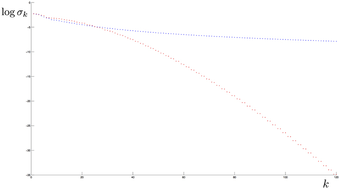
Figure 1. Eigenvalues in logarithmic scale of the Covariance operator when the kernel is Abel (blue) and Gaussian (red) and the distribution is uniformly supported on the “8” curve in Figure 2. Note that the eigenvalue decay rate of the first operator has a polynomial behavior while the second has an exponential one.

2.3. Filter Function

The second building block is a low pass filter, we introduce to avoid that the estimator overfits the empirical data. The filter functions were first introduced in the context of inverse problem, see Engl et al. [28] and references therein, and in the context of supervised learning, see Lo Gerfo et al. [29] and Blanchard and Mucke [30].

We now fix some notations. For any $f\in {H}$, we denote by f ⊗ f the rank one operator (f ⊗ f)g = 〈gf〉f. We recall that a bounded operator A on ${H}$ is a Hilbert-Schmidt operator if for some (any) basis {f_j}_j the series $\left|\right|A|{|}_2^2:=\sum _j|\left|A{f}_j\right|{|}^2$ is finite, ||A||₂ is called the Hilbert-Schmidt norm and ||A||_∞ ≤ ||A||₂, where ||·||_∞ is the spectral norm. We denote by ${{S}}_2$ the space of Hilbert-Schmidt operators, which is a separable Hilbert space under the scalar product ${\langle AB\rangle }_2=\sum _j\langle A{f}_{j}B{f}_j\rangle$.

Assumption 2. A filter function is a sequence of functions r_m:[0, R] → [0, 1], with m ∈ ℕ, satisfying

(H4) for any m ∈ ℕ, r_m(0) = 0;

(H5) for all σ > 0, ${\displaystyle \underset{m\to +\infty }{lim}}{r}_m(\sigma )=1$;

(H6) for all m ∈ ℕ, there is L_m > 0 such that

$|r_m({\sigma }^{\prime })-r_m(\sigma )|\le L_m|{\sigma }^{\prime }-\sigma |,$

i.e., r_m is a Lipschitz function with Lipschitz constant L_m.

For fixed m, r_m is a filter cutting the smallest eigenvalues (high frequencies). Indeed, (H4) and (H6) with σ′ = 0 give

$\begin{array}{cc}|r_m(\sigma )|\le L_m\left|\sigma \right|.& \left(5\right)\end{array}$

On the contrary, if m goes to infinity, by (H5) r_m converges point-wisely to the Heaviside function

$\Theta (\sigma )=\{\begin{array}{ll}1\hfill & \sigma >0\hfill \\ 0\hfill & \sigma =0\hfill \end{array}.$

Since r_m(σ) converges to Θ(σ), which does not satisfy (5), we have that $\underset{m\to +\infty }{lim}{L}_m=+\infty$.

We fix the interval [0, R] as domain of the filter functions r_m since the eigenvalues of the operators we are interested belong to [0, R], see (23).

Examples of filter functions are

• Tikhonov filter

$r_m(\sigma )=\frac{m\sigma }{m\sigma +R}{L}_m=\frac{m}{R}.$

• Soft cut-off

$r_m(\sigma )=\{\begin{array}{cc}1& \sigma \ge \frac{R}{m}\\ \frac{m\sigma }{R}& \sigma <\frac{R}{m}\end{array}{L}_m=\frac{m}{R}.$

• Landweber iteration

$r_m(\sigma )=\frac{\sigma }{R}{\displaystyle \sum _{k=0}^m{(1-\frac{\sigma }{R})}^k=1-{(1-\frac{\sigma }{R})}^{m+1}{L}_m=\frac{m+1}{R}.}$

We recall a technical result, which is based on functional calculus for compact operators. If A is a positive Hilbert-Schmidt operator, Hilbert-Schmidt theorem (for compact self-adjoint operators) gives that there exist a basis {f_j}_j of ${H}$ and a family {σ_j}_j of positive numbers such that

$\begin{array}{cc}A={\displaystyle \sum _j{\sigma }_j}{f}_j\otimes f_j\iff A{f}_j={\sigma }_j{f}_j.& \left(6\right)\end{array}$

If the spectral norm ||A||_∞ ≤ R, then all the eigenvalues σ_j belong to [0, R] and the spectral calculus defines r_m(A) as the operator on ${H}$ given by

$r_m(A)={\displaystyle \sum _j{r}_m}({\sigma }_j)f_j\otimes f_j\iff r_m(A)f_j=r_m({\sigma }_j)f_j.$

With this definition each f_j is still an eigenvector of r_m(A), but the corresponding eigenvalue is shrunk to r_m(σ_j). Proposition 1 in the Appendix in Supplementary Material summarizes the main properties of r_m(A).

2.4. Kernel Principal Component Analysis

As anticipated in the introduction, the estimators we propose are a generalization of KPCA suggested by Hoffmann [16] in the context of novelty detection. In our framework this corresponds to the hard cut-off filter, i.e., by labeling the different eigenvalues of A in a decreasing order¹ σ₁ > σ₂ > … > σ_m > σ_m+1 > …, the filter function is

$r_m(\sigma )=\{\begin{array}{ll}1\hfill & \sigma \ge {\sigma }_m\hfill \\ 0\hfill & \sigma <{\sigma }_m\hfill \end{array}.$

Clearly, r_m satisfies (H4) and (H5), but (H6) does not hold. However, the Lipschitz assumption is needed only to prove the bound (21e) and, for the hard cut-off filter, r_m(A) is simply the orthogonal projector onto the linear space spanned by the eigenvectors whose eigenvalues are bigger than σ_m+1. For such projections [37] proves the following bound

$\left|\right|r_m(A^{\prime })-r_m(A)|{|}_2\le \frac{2}{{\sigma }_{m+1}-{\sigma }_m}||A^{\prime }-A|{|}_2,$

so that (21e) holds true with $L_m=\frac{2}{{\sigma }_{m+1}-{\sigma }_m}$. Hence, our results also hold for hard cut-off filter at the price to have a Lipschitz constant L_m depending on the eigenvalues of A.

2.5. Covariance Operators

The third building block is made of the eigenvectors of the distribution dependent covariance operator and of its empirical version. The covariance operators are computed by first mapping the data in the feature space ${H}$.

As usual, we introduce two random variables Φ(X) and Φ(X) ⊗ Φ(X), taking value in ${H}$ and in ${{S}}_2$, respectively. Since Φ is continuous and X belongs to the compact subset ${D}$, both random variables are bounded. We set

$\begin{array}{ll}\mu =𝔼[\Phi (X)]={\displaystyle \underset{{D}}{\int }\Phi }(x)dP(x),& (7\text{a})\end{array}$

$\begin{array}{ll}T=𝔼[\Phi (X)\otimes \Phi (X)]={\displaystyle \underset{{D}}{\int }\Phi }(x)\otimes \Phi (x)dP(x),& (7\text{b})\end{array}$

$\begin{array}{ll}{T}^c=T-\mu \otimes \mu ,& (7\text{c})\end{array}$

where the integrals are in the Bochner sense.

We denote by ${\hat{\mu }}_n$ and ${\hat{T}}_n$ the empirical mean of Φ(X) and Φ(X) ⊗ Φ(X), respectively, and by $\widehat{T_n^c}$ the empirical covariance operator, respectively. Explicitly,

$\begin{array}{ll}{\widehat{\mu }}_n=\frac{1}{n}{\displaystyle \sum _i\Phi }(X_i),& (8\text{a})\end{array}$

$\begin{array}{ll}{\widehat{T}}_n=\frac{1}{n}{\displaystyle \sum _i\Phi }(X_i)\otimes \Phi (X_i),& (8\text{b})\end{array}$

$\begin{array}{ll}\widehat{T_n^c}={\widehat{T}}_n-{\widehat{\mu }}_n\otimes {\widehat{\mu }}_n.& (8\text{c})\end{array}$

The main properties of the covariance operator and its empirical version are summarized in Proposition 2 in the Appendix in Supplementary Material.

3. The Estimator

Now we are ready to construct the estimator, whose computational aspects are discussed in section 5. The set ${\hat{C}}_n$ is defined by the following three steps:

a) the points $x\in {D}$ are mapped into the corresponding centered vectors $\Phi (x)-{\hat{\mu }}_n\in {H}$, where the center is the empirical mean;

b) the operator $r_m(\widehat{T_n^c})$ is applied to each vector $\Phi (x)-{\hat{\mu }}_n$;

c) the point $x\in {D}$ is assigned to ${\hat{C}}_n$ if the distance between $r_{m_n}({\hat{T}}_n^c)(\Phi (x)-{\hat{\mu }}_n)$ and $\Phi (x)-{\hat{\mu }}_n$ is smaller than a threshold τ.

Explicitly we have that

$\begin{array}{ll}{\widehat{C}}_n=\{x\in {D}\mid ||r_{m_n}({\widehat{T}}_n^c)(\Phi (x)-{\widehat{\mu }}_n)-(\Phi (x)-{\widehat{\mu }}_n)||\le {\tau }_n\},& (9)\end{array}$

where τ = τ_n and m = m_n are chosen as a function of the number n of training data.

With the choice of the hard cut-off filter, this reduces to the KPCA algorithm [16, 17]. Indeed, $r_m({\hat{T}}_n^c)$ is the projection Q^m onto the vector space spanned by the first m eigenvectors. Hence ${\hat{C}}_n$ is the set of points x whose image $\Phi (x)-{\hat{\mu }}_n$ is close to Q^m. For an arbitrary filter function r_m, Q^m is replaced by $r_m({\hat{T}}_n^c)$, which can be interpreted as a smooth version of Q^m. Note that, in general, $r_m({\hat{T}}_n^c)$ is not a projection.

In De Vito et al. [27] a different estimator is defined. In that paper the data are mapped in the feature space ${H}$ without centering the points with respect to the empirical mean and the estimator is given by

${\tilde{C}}_n=\{x\in {D}\mid |\langle \Phi (x)-r_{m_n}({\widehat{T}}_n)\Phi (x)\Phi (x)\rangle |\le {\tau }_n^2\},$

where the filter function r_m is as in the present work, but $r_{m_n}({\hat{T}}_n)$ is defined in terms of the eigenvectors of the non-centered second momentum ${\hat{T}}_n$. To compare the two estimators note that

$\begin{array}{l}\left|\right|r_m({\widehat{T}}_n^c)(\Phi (x)-{\widehat{\mu }}_n)-(\Phi (x)-{\widehat{\mu }}_n)|{|}^2\\ =\langle {(I-r_m({\widehat{T}}_n^c))}^2(\Phi (x)-{\widehat{\mu }}_n)\Phi (x)-{\widehat{\mu }}_n\rangle \\ =\langle (I-r_m^{\ast }({\widehat{T}}_n^c))(\Phi (x)-{\widehat{\mu }}_n)\Phi (x)-{\widehat{\mu }}_n\rangle ,\end{array}$

where $r_m^{*}(\sigma )=2r_m(\sigma )-r_m{(\sigma )}^2$, which is a filter function too, possibly with a Lipschitz constant $L_m^{*}\le 2L_m$. Note that for the hard cut-off filter $r_m^{*}(\sigma )=r_m(\sigma )$.

Though $r_{m_n}({\hat{T}}_n)$ and $r_{m_n}({\hat{T}}_n^c)$ are different, both ${\hat{C}}_n$ and ${\tilde{C}}_n$ converge to the support of the probability distribution P, provided that the separating property (H3) holds true. Hence, one has the freedom to choose if the empirical data have or not zero mean in the feature space.

4. Main Results

In this section, we prove that the estimator ${\hat{C}}_n$ we introduce is strongly consistent. To state our results, for each n ∈ ℕ, we fix an integer m_n ∈ ℕ and set ${\hat{F}}_n:{D}\to {H}$ to be

${\widehat{F}}_n(x)=(I-r_{m_n}({\widehat{T}}_n^c))(\Phi (x)-{\widehat{\mu }}_n),$

so that Equation (9) becomes

$\begin{array}{ll}{\widehat{C}}_n=\{x\in {D}\mid ||{\widehat{F}}_n(x)||\le {\tau }_n\}.& (10\end{array}$

4.1. Spectral Characterization

First of all, we characterize the support of P by means of Q^c, the orthogonal projector onto the null space of the distribution dependence covariance operator T^c. The following theorem will show that the centered feature map

${\Phi }^c:{D}\to {H}{\Phi }^c(x)=\Phi (x)-\mu$

sends the support C onto the intersection of ${\Phi }^c({D})$ and the closed subspace $(I-Q^c){H}$, i.e,

${\Phi }^c(C)={\Phi }^c({D})\cap (I-Q^c){H}.$

Theorem 1. Assume that Φ is a separating Mercer feature map, then

$\begin{array}{ll}C=\{x\in {D}\mid Q^c(\Phi (x)-\mu )=0\},& (11)\end{array}$

where Q^c is the orthogonal projector onto the null space of the covariance operator T^c.

Proof. To prove the result we need some technical lemmas, we state and prove in the Appendix in Supplementary Material. Assume first that $x\in {D}$ is such that Q^c(Φ(x) − μ) = 0. Denoted by Q the orthogonal projection onto the null space of T, by Lemma 2 QQ^c = Q and Qμ = 0, so that

$Q\Phi (x)=Q(\Phi (x)-\mu )=Q{Q}^c(\Phi (x)-\mu )=0.$

Hence Lemma 1 implies that x ∈ C.

Conversely, if x ∈ C, then as above Q(Φ(x) − μ) = 0. By Lemma 2 we have that Q^c(1 − Q) = ||Q^cμ||⁻²Q^c μ ⊗ Q^cμ. Hence it is enough to prove that

$\langle Q^c\mu \Phi (x)-\mu \rangle =0\iff Q^c\Phi (x)=Q^c\mu ,$

which holds true by Lemma 3.

4.2. Consistency

Our first result is about the convergence of ${\hat{F}}_n$.

Theorem 2. Assume that Φ is a Mercer feature map. Take the sequence {m_n}_n such that

$\begin{array}{ll}\underset{n\to \infty }{\lim }{m}_n=+\infty ,& (12\text{a})\end{array}$

$\begin{array}{ll}{L}_{m_n}\le \kappa \frac{\sqrt{n}}{\ln n},& (12\text{b})\end{array}$

for some constant κ > 0, then

$\begin{array}{ll}\mathbb{P}\left[\underset{n\to \infty }{\lim }\underset{x\in {D}}{\sup }\right||{\widehat{F}}_n(x)-Q^c(\Phi (x)-\mu )||=0]=1.& (13)\end{array}$

Proof. We first prove Equation (13). Set $A_n=I-r_{m_n}(\widehat{T_n^c})$. Given $x\in {D}$,

$\begin{array}{l}\left|\right|A_n(\Phi (x)-{\widehat{\mu }}_n)-Q^c(\Phi (x)-\mu )\left|\right|\\ \le \left|\right|(A_n-Q^c)(\Phi (x)-\mu )\left|\right|+\left|\right|A_n(\mu -{\widehat{\mu }}_n)\left|\right|\\ \le \left|\right|r_{m_n}({\widehat{T}}_n^c)-r_{m_n}(T^c)\left|{|}_2\right||\Phi (x)-\mu ||\\ +\left|\right|(r_{m_n}(T^c)-(I-Q^c))(\Phi (x)-\mu )\left|\right|+\left|\right|A_n(\mu -{\widehat{\mu }}_n)\left|\right|\\ \le 2\sqrt{R}{L}_{m_n}\left|\right|{\widehat{T}}_n^c-T^c|{|}_2\\ +\left|\right|(r_{m_n}(T^c)-(I-Q^c))(\Phi (x)-\mu )\left|\right|+\left|\right|\mu -{\widehat{\mu }}_n\left|\right|,\end{array}$

where the fourth line is due to (21e), the bound $\left|\right|A_n|{|}_{\infty }=\underset{\sigma \in \left[0,1\right]}{sup}|1-r_m(\sigma )|\le 1$, and the fact that both Φ(x) and μ are bounded by $\sqrt{R}$. By (12b) it follows that

$\begin{array}{l}\underset{x\in {D}}{\sup }\left|\right|A_n(\Phi (x)-{\widehat{\mu }}_n)-Q^c(\Phi -\mu )\left|\right|\le 2\sqrt{R}\kappa \frac{\sqrt{n}}{\ln n}\left|\right|{\widehat{T}}_n^c-T^c|{|}_2\\ +\underset{x\in {D}}{\sup }\left|\right|(r_{m_n}(T^c)-(I-Q^c))(\Phi (x)-\mu )\left|\right|-\left|\right|\mu -{\widehat{\mu }}_n\left|\right|,\end{array}$

so that, taking into account (24a) and (24c), it holds that

$\underset{n\to +\infty }{\lim }\underset{x\in {D}}{\sup }\left|\right|A_n(\Phi (x)-{\widehat{\mu }}_n)-Q^c(\Phi -\mu )\left|\right|=0$

almost surely, provided that lim_n→+∞∥(r_mn(T^c) − (I − Q^c))(Φ(x) − μ)∥ = 0. This last limit is a consequence of (21d) observing that $\left\{\Phi (x)-\mu \mid x\in {D}\right\}$ is compact since ${D}$ is compact and Φ is continuous.

We add some comments. Theorem 1 suggests that the consistency depends on the fact that the vector $(I-r_{m_n}({\hat{T}}_n^c))(\Phi (x)-{\hat{\mu }}_n)$ is a good approximation of Q^c(Φ(x)−μ). By the law of large numbers, ${\hat{T}}_n$ and ${\hat{\mu }}_n$ converge to T and μ, respectively, and Equation (21d) implies that, if m is large enough, (I − r_m(T))(Φ(x)−μ) is closed to Q^c(Φ(x)−μ). Hence, if m_n is large enough, see condition (12a), we expect that $r_{m_n}({\hat{T}}_n^c)$ is close to $r_{m_n}(T^c)$. However, this is true only if m_n goes to infinity slowly enough, see condition (12b). The rate depends on the behavior of the Lipschitz constant L_m, which goes to infinity if m goes to infinity. For example, for Tikhonov filter a sufficient condition is that $m_n~n^{\frac{1}{2}-ϵ}$ with ϵ > 0. With the right choice of m_n, the empirical decision function ${\hat{F}}_n$ converges uniformly to the function F(x) = Q^c(Φ(x) − μ), see Equation (13).

If the map Φ is separating, Theorem 1 gives that the zero level set of F is precisely the support C. However, if C is not learnable by Φ, i.e., the equality (2) does not hold, then the zero level set of F is bigger than C. For example, if ${D}$ is connected, C has not-empty interior and Φ is the feature map associated with the Gaussian kernel, it is possible to prove that F is an analytic function, which is zero on an open set, hence it is zero on the whole space ${D}$. We note that, in real applications the difference between Gaussian and Abel kernel, which is separating, is not so big and in our experience the Gaussian kernel provides a reasonable estimator.

From now on we assume that Φ is separating, so that Theorem 1 holds true. However, the uniform convergence of ${\hat{F}}_n$ to F does not imply that the zero level sets of ${\hat{F}}_n$ converges to C = F⁻¹(0) with respect to the Hausdorff distance. For example, with the Tikhonov filter ${\hat{F}}_n^{-1}(0)$ is always the empty set. To overcome the problem, ${\hat{C}}_n$ is defined as the τ_n-neighborhood of the zero level set of ${\hat{F}}_n$, where the threshold τ_m goes to zero slowly enough.

Define the data dependent parameter ${\hat{\tau }}_n$ as

$\begin{array}{ll}{\widehat{\tau }}_n=\underset{1\le i\le n}{\max }\left|\right|{\widehat{F}}_n(X_i)\left|\right|.& (14)\end{array}$

Since ${\hat{F}}_n\in \left[0,1\right]$, clearly ${\hat{\tau }}_n\in \left[0,1\right]$ and the set estimator becomes

${\widehat{C}}_n=\{x\in {D}\mid ||{\widehat{F}}_n(x)||\le {\widehat{\tau }}_n\}.$

The following result shows that ${\hat{C}}_n$ is a universal strongly consistent estimator of the support of the probability distribution P. Note that for KPCA the consistency is not universal since the choice of m_n depends on some a-priori information about the decay of the eigenvalues of the covariance operator T^c, which depends on P.

Theorem 3. Assume that Φ is a separating Mercer feature map. Take the sequence {m_n}_n satisfying (12a)-(12b) and define ${\hat{\tau }}_n$ by (14). Then

$\begin{array}{ll}\mathbb{P}[\underset{n\to \infty }{\lim }{\widehat{\tau }}_n=0]=1,& (15\text{a})\end{array}$

$\begin{array}{ll}\mathbb{P}[\underset{n\to \infty }{\lim }{d}_{{}_H}({\widehat{C}}_n,C)=0]=1.& (15\text{b})\end{array}$

Proof. We first show Equation (15a). Set F(x) = Q^c(Φ(x) − μ) and let E be the event on which ${\hat{F}}_n$ converges uniformly to F(x), and F be the event such that X_i ∈ C for all i ≥ 1. Theorem 2 shows that ℙ[E] = 1 and, since C is the support, then ℙ[F] = 1. Take ω ∈ E ∩ F and fix ϵ > 0, then there exists n₀ > 0 (possibly depending on ω and ϵ) such that for all n ≥ n₀ $|{\hat{F}}_n(x)-F(x)|\le ϵ$ for all $x\in {D}$. By Theorem 1 F(x) = 0 for all x ∈ C and X₁(ω), …, X_n(ω) ∈ C, it follows that $\left|{\hat{F}}_n(X_i(\omega ))\right|\le ϵ$ for all 1 ≤ i ≤ n so that $0\le {\hat{\tau }}_n(\omega )\le ϵ$, so that the sequence ${\hat{\tau }}_n(\omega )$ goes to zero. Since ℙ[E ∩ F] = 1 Equation (15a) holds true.

We split the proof of Equation (15b) in two steps. We first show that with probability one $\underset{n\to +\infty }{lim}\underset{x\in {\hat{C}}_n}{sup}d(x,C)=0$. On the event E ∩ F, suppose, by contraction, that the sequence ${\left\{{sup}_{x\in {\hat{C}}_n}\mathrm{\text{d}}(x,C)\right\}}_n$ does not converge to zero. Possibly passing to a subsequence, for all n ∈ ℕ there exists $x_n\in {\hat{C}}_n$ such that $d(x_n,{\hat{C}}_n)\ge {ϵ}_0$ for some fixed ϵ₀ > 0. Since ${D}$ is compact, possibly passing to a subsequence, {x_n}_n converges to $x_0\in {D}$ with d(x₀, C) ≥ ϵ₀. We claim that x₀ ∈ C. Indeed,

$\begin{array}{l}\left|\right|Q^c(\Phi (x_0)-\mu )\left|\right|\le \left|\right|Q^c(\Phi (x_0)-\Phi (x_n))\left|\right|\\ +\left|\right|{\widehat{F}}_n(x_n)-Q^c(\Phi (x_n)-\mu )\left|\right|+\left|\right|{\widehat{F}}_n(x_n)\left|\right|\\ \le \left|\right|Q^c(\Phi (x_0)-\Phi (x_n))\left|\right|\\ +\underset{x\in {D}}{\sup }\left|\right|{\widehat{F}}_n(x)-Q^c(\Phi (x)-\mu )+{\tau }_n,\end{array}$

since $x_n\in {\hat{C}}_n$ means that $\left|\right|{\hat{F}}_n(x_n)\left|\right|\le {\tau }_n$. If n goes to infinity, since Φ is continuous and by the definition of E and F, the right side of the above inequality goes to zero, so that $\left|\right|Q^c(\Phi (x_0)-\mu )\left|\right|=0$, i.e., by Theorem 1 we get x₀ ∈ C, which is a contraction since by construction d(x₀, C) ≥ ϵ₀ > 0.

We now prove that

$\underset{n\to \infty }{\lim }\underset{x\in C}{\sup }\text{d}(x,{\widehat{C}}_n).$

For any $x\in {D}$, set X_1,n(x) to be a first neighbor of x in the training set {X₁, …, X_n}. It is known that for all x ∈ C,

$\begin{array}{ll}\mathbb{P}\left[\underset{n\to +\infty }{\lim }\text{d}(X_{1,n}(x),x)=0\right]=1,& (16)\end{array}$

see for example Lemma 6.1 of Györfi et al. [35].

Choose a denumerable family {z_j}_{j ∈ J} in C such that is dense in C. By Equation (16) there exists an event G with such that ℙ[G] = 1 and, on G, for all j ∈ J

$\underset{n\to +\infty }{\lim }\text{d}(X_{1,n}(z_j),z_j)=0.$

Fix ω ∈ G, we claim that $\underset{n}{lim}{sup}_{x\in C}\mathrm{\text{d}}(x,{\hat{C}}_n)=0$. Observe that, by definition of ${\hat{\tau }}_n$, $X_i\in {\hat{C}}_n$ for all 1 ≤ i ≤ n and

$\underset{x\in C}{\sup }\text{d}(x,{\widehat{C}}_n)\le \underset{x\in C}{\sup }\underset{1\le i\le n}{\min }\text{d}(x,X_i)=\underset{x\in C}{\sup }\text{d}(X_{1,n}(x),x),$

so that it is enough to show that ${\lim }_{n\to +\infty }{\text{sup}}_{x\in C}\text{d}\left(X_{1,n}(x),x\right)=0$.

Fix ϵ > 0. Since C is compact, there is a finite subset J_ϵ ⊂ J such that {B(z_j, ϵ)}_{j ∈ Jϵ} is a finite covering of C. Furthermore,

$\begin{array}{ll}\underset{x\in C}{\sup }\text{d}(X_{1,n}(x),x)\le \underset{j\in J_{ϵ}}{\max }\text{d}(X_{1,n}(z_j),z_j)+ϵ.& (17)\end{array}$

Indeed, fix x ∈ C, there exists an index j ∈ J_ϵ such that x ∈ B(z_j, ϵ). By definition of first neighbor, clearly

$\text{d}(X_{1,n}(x),x)\le \text{d}(X_{1,n}(z_j),x),$

so that by triangular inequality we get

$\begin{array}{l}\text{d}(X_{1,n}(x),x)\le \text{d}(X_{1,n}(z_j),x)\le \text{d}(X_{1,n}(z_j),z_j)+\text{d}(z_j,x)\\ \le \text{d}(X_{1,n}(z_j),z_j)+ϵ\\ \le \underset{j\in J_{ϵ}}{\max }\text{d}(X_{1,n}(z_j),z_j)+ϵ.\end{array}$

Taking the supremum over C we get the claim. Since ω ∈ G and J_ϵ is finite,

$\underset{n\to +\infty }{\lim }\underset{j\in J_{ϵ}}{\max }\text{d}(X_{1,n}(z_j),z_j)=0,$

so that by Equation (17)

$\underset{n\to +\infty }{\text{limsup }}\underset{x\in C}{\sup }\text{d}(X_{1,n}(x),x)\le ϵ.$

Since ϵ is arbitrary, we get $\underset{n\to +\infty }{lim}{sup}_{x\in C}\mathrm{\text{d}}(X_{1,n}(x),x)=0$, which implies that

$\underset{n\to +\infty }{\lim }\underset{x\in C}{\sup }\text{d}(x,{\widehat{C}}_n)=0.$

Theorem 3 is an asymptotic result. Up to now, we are not able to provide finite sample bounds on d_H(Ĉ_n, C). It is possible to have finite sample bounds on $\left|\right|{\hat{F}}_n(x)-Q^c(\Phi (x)-\mu )\left|\right|$, as in Theorem 7 of De Vito et al. [25] with the same kind of proof.

4.3. The Separating Condition

The following two examples clarify the notion of the separating condition.

Example 1. Let ${D}$ be a compact subset of ℝ², ${H}={ℝ}^6$ with the euclidean scalar product, and $\Phi :{D}\to {ℝ}^6$ be the feature map

$\Phi ((x,y))=(x^2,y^2,\sqrt{2}xy,\sqrt{2}x,\sqrt{2}y,1),$

whose corresponding Mercer kernel is a polynomial kernel of degree two, explicitly given by

$K\left(x_1,y_1;x_2,y_2\right)={\left(x_1{x}_2+y_1{y}_2+1\right)}^2.$

Given a vector $f={(f_1,\dots ,f_6)}^{\top }$, the corresponding elementary set is the conic

$\begin{array}{l}{C}_{f,c}=\{(x,y)\in {D}\mid f_1{x}^2+f_2{y}^2+f_3\sqrt{2}xy\\ +f_4\sqrt{2}x+f_5\sqrt{2}y+f_6=0\},\end{array}$

Conversely, all the conics are elementary sets. The family of all the intersections of at most five conics, i.e., the sets whose cartesian equation is a system of the form

$\{\begin{array}{l}{f}_{11}{x}^2+f_{12}{y}^2+f_{13}\sqrt{2}xy+f_{14}\sqrt{2}x+f_{15}\sqrt{2}y+f_{16}=0\hfill \\ ⋮\hfill \\ f_{51}{x}^2+f_{52}{y}^2+f_{53}\sqrt{2}xy+f_{54}\sqrt{2}x+f_{55}\sqrt{2}y+f_{56}=0\hfill \end{array},$

where f₁₁, …, f₅₆ ∈ ℝ.

Example 2. The data are the random vectors in ℝ²

$X_i=(\sin (a{\Theta }_i+b),\sin (c{\Theta }_i+d)),$

where a, c ∈ ℕ, b, d ∈ [0, 2π] and Θ₁, …, Θ_n are independent random variables, each of them uniformly distributed on [0, 2π]. Setting ${D}={\left[-1,1\right]}^2$, clearly $X_i\in {D}$ and the support of their common probability distribution is the Lissajous curve

$C={\text{Lis}}_{a,b,c,d}=\{(\sin (a\theta +b),\sin (c\theta +d))\in {D}\mid \theta \in [0,2\pi ]\}.$

Figure 2 shows two examples of Lissajous curves. As a filter function r_m, we fix the hard cut-off filter where m is the number of eigenvectors corresponding to the highest eigenvalues we keep. We denote by ${Ĉ}_n^{m,\tau }$ the corresponding estimator given by (10).

FIGURE 2

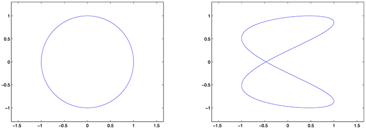
Figure 2. Examples of Lissajous curves for different values of the parameters. (Left) ${\mathrm{\text{Lis}}}_{1,0,1,\frac{\pi }{2}}$. (Right) Lis_2,0.11,1,0.3.

In the first two tests we use the polynomial kernel (18), so that the elementary learnable sets are conics. One can check that the rank of T^c is less or equal than 5. More precisely, if Lis_a,b,c,d is a conic, the rank of T^c is 4 and we need to estimate five parameters, whereas if Lis_a,b,c,d is not a conic, Lis_a,b,c,d is not a learnable set and the rank of T^c is 5.

In the first test the data are sampled from the distribution supported on the circumference ${\mathrm{\text{Lis}}}_{1,0,1,\frac{\pi }{2}}$ (see panel left of Figure 2). In Figure 3 we draw the set ${Ĉ}_n^{m,\tau }$ for different values of m and τ when n varies. In this toy example n = 5 is enough to learn exactly the support, hence for each n = 2, …, 5 the corresponding values of m_n and τ_n are m_n = 1, 2, 3, 4 and τ_n = 0.01, 0.005, 0.005, 0.002.

FIGURE 3

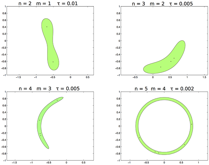
Figure 3. From left to right, top to bottom. The set ${Ĉ}_n^{m,\tau }$ with n, respectively 2, 3, 4, 5, m = 1, 2, 3, 4 and τ = 0.1, 0.005, 0.005, 0.002.

In the second test the data are sampled from the distribution supported on the curve Lis_2,0.11,1,0.3, which is not a conic (see panel right of Figure 2). In Figure 4 we draw the set ${Ĉ}_n^{m,\tau }$ for n = 10, 20, 50, 100, m = 4, and τ = 0.01. Clearly, ${\hat{C}}_n$ is not able to estimate Lis_2,0.11,1,0.3.

FIGURE 4

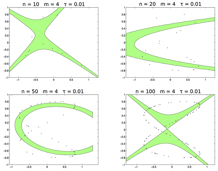
Figure 4. The set ${Ĉ}_n^{4,0.01}$ with n respectively 10, 20, 50, 100.

In the third test, we use the Abel kernel with the data sampled from the distribution supported on the curve Lis_2,0.11,1,0.3 (see panel right of Figure 2). In Figure 5 we show the set ${Ĉ}_n^{m,\tau }$ for n = 20, 50, 100, 500, m = 5, 20, 30, 50, and τ = 0.4, 0.35, 0.3, 0.2. According the fact that the kernel is separating, ${\hat{C}}_n$ is able to estimate Lis_2,0.11,1,0.3 correctly.

FIGURE 5

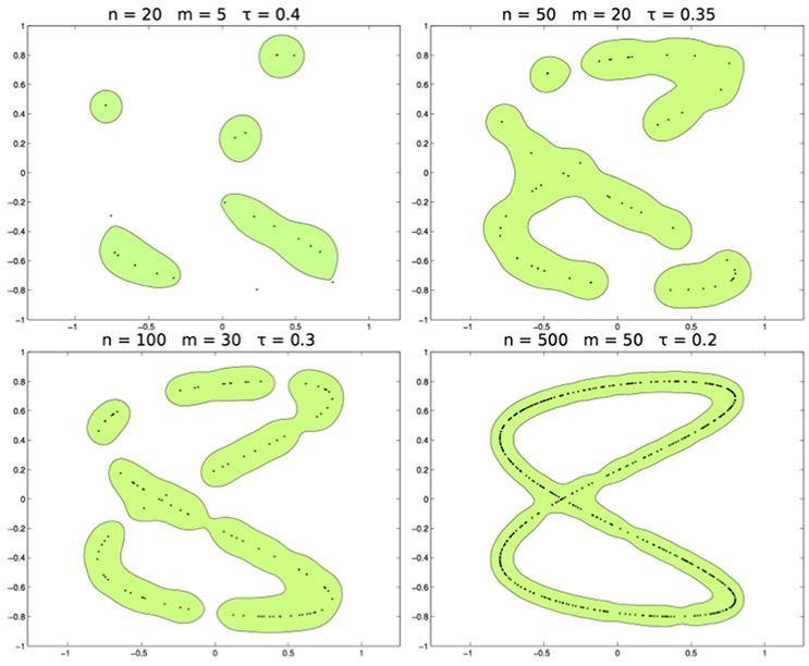
Figure 5. From left to right and top to bottom. The learned set ${Ĉ}_n^{m,\tau }$ with n respectively of 20, 50, 100, 500, and m = 5, 20, 30, 50, τ = 0.4, 0.35, 0.3, 0.2.

We now briefly discuss how to select the parameter m_n and τ_n from the data. The goal of set-learning problem is to recover the support of the probability distribution generating the data by using the given input observations. Since no output is present, set-learning belongs to the category of unsupervised learning problems, for which there is not a general framework accounting for model selection. However there are some possible strategies (whose analysis is out of the scope of this paper). A first approach, we used in our simulations, is based on the monotonicity properties of ${Ĉ}_n^{m,\tau }$ with respect to m, τ. More precisely, given f ∈ (0, 1), we select (the smallest) m and (the biggest) τ such that at most nf observed points belong to the the estimated set. It is possible to prove that this method is consistent when f tends to 1 as the number of observations increases. Another way to select the parameters consists in transforming the set-learning problem is a supervised one and then performing standard model selection techniques like cross validation. In particular set-learning can be casted in a classification problem by associating the observed example to the class +1 and by defining an auxiliary measure μ (e.g., uniform on a ball of interest in ${D}$) associated to −1, from which n i.i.d. points are drawn. It is possible to prove that this last method is consistent when μ(suppρ) = 0.

4.4. The Role of the Regularization

We now explain the role of the filter function. Given a training set X₁, …, X_n of size n, the separating property (3) applied to the support of the empirical distribution gives that

$\{X_1,\dots ,X_n\}=\{x\in {D}\mid \widehat{Q_n^c}(\Phi (x)-{\widehat{\mu }}_n)=0\},$

where ${\hat{\mu }}_n$ is the empirical mean and $I-\widehat{Q_n^c}$ is the orthogonal projection onto the linear space spanned by the family $\left\{\Phi (X_1)-{\hat{\mu }}_n,\dots ,\Phi (X_n)-{\hat{\mu }}_n\right\}$, which are the centered images of the examples. Hence, given a new point x ∈ D the condition $|\widehat{Q_n^c}(\Phi (x)-{\widehat{\mu }}_n)||\le \tau$ with τ ≪ 1 is satisfied if only if x is close to one of the examples in the training set. Hence the naive estimator $\left\{x\in {D}|\Vert \widehat{Q_n^c}\left(\Phi \left(x\right)-\widehat{{\mu }_n}\right)\Vert \le \tau \right\}$ overfits the data. Hence we would like to replace $\widehat{Q_n^c}$ with an operator, which should be close to the identity on the linear subspace spanned by $\left\{\Phi (X_1)-{\hat{\mu }}_n,\dots ,\Phi (X_n)-{\hat{\mu }}_n\right\}$ and it should have a small range. To modulate the two requests, one can consider the following optimization problem

$\underset{A\in S_2}{\min }\left(\frac{1}{n}{\displaystyle \sum _{i=1}^n{\Vert (I-A)(\Phi (X_i)-{\widehat{\mu }}_n)\Vert }^2+\lambda {\Vert A\Vert }_2^2}\right).$

We note that if A is a projection its Hilbert-Schmidt norm ||A||₂ is the square root of the dimension of the range of A. Since

$\begin{array}{l}\frac{1}{n}{\displaystyle \sum _{i=1}^n\left|\right|}(I-A)(\Phi (X_i)-{\widehat{\mu }}_n)|{|}^2\\ =\text{Tr}\left(\left(I-A^{\top }\right)\left(I-A\right)\right)\frac{1}{n}{\displaystyle \sum _{i=1}^n\left(\Phi (X_i)-{\widehat{\mu }}_n)\otimes (\Phi (X_i)-{\widehat{\mu }}_n)\right)}\\ =\text{Tr}\left(\left(I-A^{\top }\right)\left(I-A\right)\stackrel{⌢}{T_n^c}\right),\end{array}$

where Tr(A) is the trace, A^⊤ is the transpose and $\left|\right|A|{|}_2=\sqrt{\mathrm{\text{Tr}}(A^{\top }A)}$ is the Hilbert-Schmidt norm, then

$\begin{array}{l}\frac{1}{n}{\displaystyle \sum _{i=1}^n\left|\right|}(I-A)(\Phi (X_i)-{\widehat{\mu }}_n)|{|}^2+\lambda |\left|A\right|{|}_2^2\\ =\text{Tr}\left((I-A^{\top })(I-A){\widehat{T}}_n^c + {\lambda }_m{A}^{\top }A\right),\end{array}$

and the optimal solution is given by

$A_{\text{opt}}=\widehat{T_n^c}{\left(\widehat{T_n^c}+{\lambda }_m\right)}^{-1},$

i.e., A_opt is precisely the operator $r_m(\widehat{T_n^c})$ with the Tikhonov filter $r_m(\sigma )=\frac{\sigma }{\sigma +\lambda }$ and $\lambda =\frac{R}{m}$. A different choice of the filter function r_m corresponds to a different regularization of the least-square problem

$\min \frac{1}{n}{\displaystyle \sum _{i=1}^n\left|\right|}(I-A)(\Phi (X_i)-{\widehat{\mu }}_n)|{|}^2.$

5. The Kernel Machine

In this section we show that the computation of $\left|\right|{\hat{F}}_n(x)\left|\right|$, in terms of which is defined the estimator ${\hat{C}}_n$, reduces to a finite dimensional problem, depending only on the Mercer kernel K, associated with the feature map. We introduce the centered sampling operator

$S_n^c:\mathscr{H}\to {ℝ}^n{\left(S_n^{c}f\right)}_i=\langle f,\Phi (X_i)-{\widehat{\mu }}_n\rangle ,$

whose transpose is given by

$S_n^c{}^{\top }:{ℝ}^n\to \mathscr{H}{S}_n^c{}^{\top }v={\displaystyle \sum _{i=1}{v}_i}(\Phi (X_i)-{\widehat{\mu }}_n),$

where v_i is the i-th entry of the column vector v ∈ ℝⁿ. Hence, it holds that

$\begin{array}{l}\frac{1}{n}{S}_n^c{}^{\top }{S}_n^c=\widehat{T_n^c},\\ \frac{1}{n}{S}_n^c{S}_n^c{}^{\top }=({\text{I}}_n-\frac{11^{\top }}{n})\frac{K_n}{n}({\text{I}}_n-\frac{11^{\top }}{n}),\end{array}$

where K_n is the n × n matrix whose (i, j)-entry is K(X_i, X_j) and I_n is the identity n × n matrix, so that the (i, j)-entry of $S_n^c{S_n^c}^{\top }$ is

$K(X_i,X_j)-\frac{1}{n}{\displaystyle \sum _{b}K}(X_i,X_b)-\frac{1}{n}{\displaystyle \sum _{a}K}(X_a,X_j)+\frac{1}{n^2}{\displaystyle \sum _{a,b}K}(X_a,X_b).$

Denoted by ℓ the rank of $S_n^c{S_n^c}^{\top }$, take the singular value decomposition of $S_n^c{S_n^c}^{\top }/n$, i.e.,

$\frac{S_n^c{S}_n^c{}^{\top }}{n}=V\Sigma V^{\top },$

where V is an n × ℓ matrix whose columns ${\text{v}}_j\in {ℝ}^n$ are the normalized eigenvectors, $V^{\top }V={\mathrm{\text{I}}}_{\ell }$, and Σ is a diagonal ℓ × ℓ matrix with the strictly positive eigenvalues on the diagonal, i.e., $\Sigma =\mathrm{\text{diag}}({\hat{\sigma }}_1,\dots ,{\hat{\sigma }}_{\ell })$. Set $U={S_n^c}^{\top }V{\Sigma }^{-\frac{1}{2}}$, regarded as operator from ℝ^ℓ to ${H}$, then a simple calculation shows that

$\widehat{T_n^c}=U\Sigma U^{\top }{r}_m(\widehat{T_n^c})=U{r}_m(\Sigma )U^{\top },$

where r_m(Σ) is the diagonal ℓ × ℓ matrix

$r_m(\Sigma )=\text{diag}(r_m({\widehat{\sigma }}_1),\dots ,r_m({\widehat{\sigma }}_{\ell })),$

and the equation for $r_m(\widehat{T_n^c})$ holds true since by assumption r_m(0) = 0. Hence

$\begin{array}{l}\left|\right|{\widehat{F}}_n(x)|{|}^2=\langle (I-r_m(\widehat{T_n^c}))(\Phi (x)-{\widehat{\mu }}_n)(I-r_m(\widehat{T_n^c}))(\Phi (x)-{\widehat{\mu }}_n)\rangle \\ =\langle \Phi (x)-{\widehat{\mu }}_n\Phi (x)-{\widehat{\mu }}_n\rangle -\langle (2r_m(\widehat{T_n^c})\\ -r_m{\left(\widehat{T_n^c}\right)}^2)(\Phi (x)-{\widehat{\mu }}_n)\rangle \Phi (x)-{\widehat{\mu }}_n\\ =\langle \Phi (x)-{\widehat{\mu }}_n\Phi (x)-{\widehat{\mu }}_n\rangle -\langle U(2r_m(\Sigma )\\ -r_m{\left(\Sigma \right)}^2)U^{\top }(\Phi (x)-{\widehat{\mu }}_n)\rangle \Phi (x)-{\widehat{\mu }}_n\\ =\langle \Phi (x)-{\widehat{\mu }}_n\Phi (x)-{\widehat{\mu }}_n\rangle -\langle V{\Sigma }^{-\frac{1}{2}}(2r_m(\Sigma )\\ -r_m{\left(\Sigma \right)}^2){\Sigma }^{-\frac{1}{2}}{V}^{\top }{S}_n^c(\Phi (x)-{\widehat{\mu }}_n)\rangle S_n^c(\Phi (x)-{\widehat{\mu }}_n)\\ =w(x)-v{\left(x\right)}^{\top }{G}_{m}v(x),& (19)\end{array}$

where the real number $w(x)=\langle \Phi (x)-{\hat{\mu }}_n\Phi (x)-{\hat{\mu }}_n\rangle$ is

$w(x)=K(x,x)-\frac{2}{n}{\displaystyle \sum _{b}K}(x,X_b)+\frac{1}{n^2}{\displaystyle \sum _{a,b}K}(X_a,X_b),$

the i-th entry of the column vector v(x) ∈ ℝⁿ is

$\begin{array}{l}v{\left(x\right)}_i={\left(S_n^c(\Phi (x)-{\widehat{\mu }}_n)\right)}_i=K(x,X_i)-\frac{1}{n}{\displaystyle \sum _{a}K}(X_a,x)\\ -\frac{1}{n}{\displaystyle \sum _{b}K}(X_i,X_b)+\frac{1}{n^2}{\displaystyle \sum _{a,b}K}(X_a,X_b),\end{array}$

the diagonal ℓ × ℓ matrix $R_m(\Sigma )={\Sigma }^{-1}(2r_m(\Sigma )-r_m{(\Sigma )}^2)$ is

$R_m(\Sigma )=\text{diag}\left(\frac{2r_m({\widehat{\sigma }}_1)-r_m{({\widehat{\sigma }}_1)}^2}{{\widehat{\sigma }}_1},\dots ,\frac{2r_m({\widehat{\sigma }}_{\ell })-r_m{({\widehat{\sigma }}_{\ell })}^2}{{\widehat{\sigma }}_{\ell }}\right),$

and the n × n-matrix G_m is

$\begin{array}{cc}{G}_m=V{R}_m(\Sigma )V^{\top }.& (20)\end{array}$

In Algorithm 1 we list the corresponding MatLab Code.

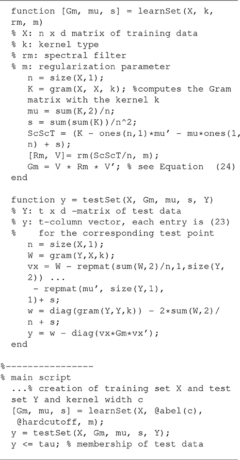
Algorithm 1. Matlab code for Set Learning.

The above equations make clear that both ${\hat{F}}_n$ and ${\hat{C}}_n$ can be computed in terms of the singular value decomposition (V, Σ) of the n × n Gram matrix K_n and of the filter function r_m, so that ${\hat{F}}_n$ belongs to the class of kernel methods and ${\hat{C}}_n$ is a plug-in estimator. For the hard cut-off filter, one simply has

$R_m{\left(\Sigma \right)}_{ii}=\{\begin{array}{ll}\frac{1}{{\widehat{\sigma }}_i}\hfill & {\widehat{\sigma }}_i\ge {\widehat{\sigma }}_m\hfill \\ 0\hfill & {\widehat{\sigma }}_i<{\widehat{\sigma }}_m\hfill \end{array}.$

For real applications, a delicate issue is the choice of the parameters m and τ, we refer to Rudi et al. [31] for a detailed discussion. Here, we add some simple remarks.

We first discuss the role of τ. According to (10), ${Ĉ}_n^{m,\tau }\subseteq {Ĉ}_n^{m,{\tau }^{\prime }}$ whenever τ < τ′. We exemplify this behavior with the dataset of Example 2. The training set is sampled from the distribution supported on the curve Lis_2,0.11,1,0.3 (see panel right of Figure 2) and we compute ${\hat{C}}_n$ with the Abel kernel, n = 100 and m ranging over 5, 10, 20, 50. Figure 6 shows the nested sets when τ runs in the associated color-bar.

FIGURE 6

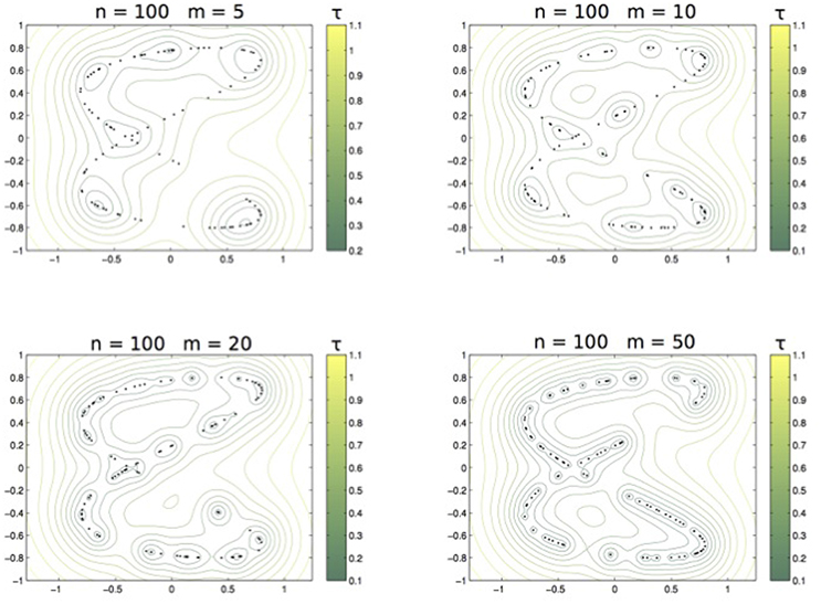
Figure 6. From left to right and top to bottom: The family of sets ${Ĉ}_{100}^{5,\tau }$,${Ĉ}_{100}^{10,\tau }$,${Ĉ}_{100}^{20,\tau }$,${Ĉ}_{100}^{50,\tau }$ with τ varying as in the related colorbar.

Analyzing the role of m, we now show that, for the the hard cut-off filter, ${Ĉ}_n^{m^{\prime },\tau }\subseteq {Ĉ}_n^{m,\tau }$ whenever m′ ≤ m. Indeed, this filter satisfies $r_{m^{\prime }}(\sigma )\le r_m(\sigma )$ and, since 0 ≤ r_m(σ) ≤ 1, one has ${(1-r_m(\sigma ))}^2\le {(1-r_{m^{\prime }}(\sigma ))}^2$. Hence, denoted by ${\left\{{\hat{u}}_j\right\}}_j$ a base of eigenvectors of $\widehat{T_n^c}$, it holds that

$\begin{array}{l}\left|\right|(I-r_m(\widehat{T_n^c}))(\Phi (x)-{\widehat{\mu }}_n)|{|}^2={\displaystyle \sum _j(1-r_m(}{\widehat{\sigma }}_j){)}^2{\langle \Phi (x)-{\widehat{\mu }}_n{\widehat{u}}_j\rangle }^2\\ \le {\displaystyle \sum _j(1-r_{m^{\prime }}(}{\widehat{\sigma }}_j){)}^2{\langle \Phi (x)-{\widehat{\mu }}_n{\widehat{u}}_j\rangle }^2\\ =\left|\right|(I-r_{m^{\prime }}(\widehat{T_n^c}))(\Phi (x)-{\widehat{\mu }}_n)|{|}^2.\end{array}$

Hence, for any point in $x\in {Ĉ}_n^{m^{\prime },\tau }$,

$\begin{array}{l}\left|\right|(I-r_m(\widehat{T_n^c}))(\Phi (x)-{\widehat{\mu }}_n)|{|}_{\mathscr{H}}^2\\ \le \left|\right|(I-r_{m^{\prime }}(\widehat{T_n^c}))(\Phi (x)-{\widehat{\mu }}_n)|{|}_{\mathscr{H}}^2\le {\tau }^2,\end{array}$

so that $x\in {Ĉ}_n^{m,\tau }$.

As above, we illustrate the different choices of m with the data sampled from the curve Lis_2,0.11,1,0.3 and the Abel kernel where n = 100 and τ ranges over 0.25, 0.3, 0.4, 0.5. Figure 7 shows the nested sets when m runs in the associated color-bar.

FIGURE 7

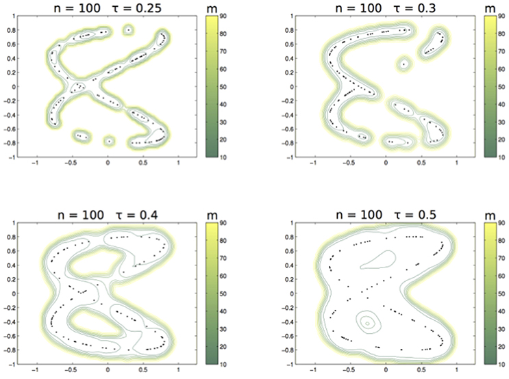
Figure 7. From left to right and top to bottom: The family of sets ${Ĉ}_{100}^{m,0.25}$,${Ĉ}_{100}^{m,0.3}$,${Ĉ}_{100}^{m,0.4}$,${Ĉ}_{100}^{m,0.5}$ with m varying as in the related colorbar.

6. Discussion

We presented a new class of set estimators, which are able to learn the support of an unknown probability distribution from a training set of random data. The set estimator is defined through a decision function, which can be seen as a novelty/anomality detection algorithm as in Schölkopf et al. [6].

The decision function we defined is a kernel machine. It is computed by the singular value decomposition of the empirical (kernel)-covariance matrix and by a low pass filter. An example of filter is the hard cut-off function and the corresponding decision function reduces to KPCA algorithm for novelty detection first introduced by Hoffmann [16]. However, we showed that it is possible to choose other low pass filters, as it was done for a class of supervised algorithms in the regression/classification setting [38].

Under some weak assumptions on the low pass filter, we proved that the corresponding set estimator is strongly consistent with respect to the Hausdorff distance, provided that the kernel satisfies a suitable separating condition, as it happens, for example, for the Abel kernel. Furthermore, by comparing Theorem 2 with a similar consistency result in De Vito et al. [27], it appears clear that the algorithm correctly learns the support both if the data have zero mean, as in our paper, and if the data are not centered, as in De Vito et al. [27]. On the contrary, if the separating property does not hold, the algorithm learns only the supports that are mapped into linear subspaces by the feature map defined by the kernel.

The set estimator we introduced depends on two parameters: the effective number m of eigenvectors defining the decision function and the thickness τ of the region estimating the support. The role of these parameters and of the separating property was briefly discussed by a few tests on toy data.

We finally observe that our class of set learning algorithms is very similar to classical kernel machines in supervised learning. So, in order to reduce both the computational cost and the memory requirements, there is the possibility to successfully implement some new advanced approximation techniques, for which there exist theoretical guarantees for the statistical learning setting. For example random features [39, 40], Nyström projections [41, 42] or mixed approaches with iterative regularization and preconditioning [43, 44].

Author Contributions

All authors listed have made a substantial, direct and intellectual contribution to the work, and approved it for publication.

Conflict of Interest Statement

The authors declare that the research was conducted in the absence of any commercial or financial relationships that could be construed as a potential conflict of interest.

Acknowledgments

ED is member of the Gruppo Nazionale per l'Analisi Matematica, la Probabilità e le loro Applicazioni (GNAMPA) of the Istituto Nazionale di Alta Matematica (INdAM).

Supplementary Material

The Supplementary Material for this article can be found online at: https://www.frontiersin.org/articles/10.3389/fams.2017.00023/full#supplementary-material

Footnotes

1. ^Here, the labeling is different from the one in (6), where the eigenvalues are repeated according to their multiplicity.

References

1. Devroye L, Wise GL. Detection of abnormal behavior via nonparametric estimation of the support. SIAM J Appl Math. (1980) 38:480–8. doi: 10.1137/0138038

CrossRef Full Text | Google Scholar

2. Korostelëv AP, Tsybakov AB. Minimax Theory of Image Reconstruction. New York, NY: Springer-Verlag (1993).

Google Scholar

3. Dümbgen L, Walther G. Rates of convergence for random approximations of convex sets. Adv Appl Probab. (1996) 28:384–93. doi: 10.2307/1428063

CrossRef Full Text | Google Scholar

4. Cuevas A, Fraiman R. A plug-in approach to support estimation. Ann Stat. (1997) 25:2300–12. doi: 10.1214/aos/1030741073

CrossRef Full Text | Google Scholar

5. Tsybakov AB. On nonparametric estimation of density level sets. Ann Stat. (1997) 25:948–69. doi: 10.1214/aos/1069362732

CrossRef Full Text | Google Scholar

6. Schölkopf B, Platt J, Shawe-Taylor J, Smola A, Williamson R. Estimating the support of a high-dimensional distribution. Neural Comput. (2001) 13:1443–71. doi: 10.1162/089976601750264965

CrossRef Full Text | Google Scholar

7. Cuevas A, Rodríguez-Casal A. Set estimation: an overview and some recent developments. In: Recent Advances and Trends in Nonparametric Statistics. Elsevier: Amsterdam (2003). p. 251–64.

8. Reitzner M. Random polytopes and the Efron-Stein jackknife inequality. Ann Probab. (2003) 31:2136–66. doi: 10.1214/aop/1068646381

CrossRef Full Text | Google Scholar

9. Steinwart I, Hush D, Scovel C. A classification framework for anomaly detection. J Mach Learn Res. (2005) 6:211–32.

Google Scholar

10. Vert R, Vert JP. Consistency and convergence rates of one-class SVMs and related algorithms. J Mach Learn Res. (2006) 7:817–54.

Google Scholar

11. Scott CD, Nowak RD. Learning minimum volume sets. J Mach Learn Res. (2006) 7:665–704.

Google Scholar

12. Biau G, Cadre B, Mason D, Pelletier B. Asymptotic normality in density support estimation. Electron J Probab. (2009) 91:2617–35.

Google Scholar

13. Cuevas A, Fraiman R. Set estimation. In: W. Kendall and I. Molchanov, editors. New Perspectives in Stochastic Geometry. Oxford: Oxford University Press (2010). p. 374–97.

14. Bobrowski O, Mukherjee S, Taylor JE. Topological consistency via kernel estimation. Bernoulli (2017) 23:288–328. doi: 10.3150/15-BEJ744

CrossRef Full Text | Google Scholar

15. Campos GO, Zimek A, Sander J, Campello RJ, Micenková B, Schubert E, et al. On the evaluation of unsupervised outlier detection: measures, datasets, and an empirical study. Data Min Knowl Discov. (2016) 30:891–927. doi: 10.1007/s10618-015-0444-8

CrossRef Full Text | Google Scholar

16. Hoffmann H. Kernel PCA for novelty detection. Pattern Recognit. (2007) 40:863–74. doi: 10.1016/j.patcog.2006.07.009

CrossRef Full Text | Google Scholar

17. Schölkopf B, Smola A, Müller KR. Nonlinear component analysis as a kernel eigenvalue problem. Neural Comput. (1998) 10:1299–319.

Google Scholar

18. Ristic B, La Scala B, Morelande M, Gordon N. Statistical analysis of motion patterns in AIS data: anomaly detection and motion prediction. In: 2008 11th International Conference on Information Fusion (2008). p. 1–7.

Google Scholar

19. Lee HJ, Cho S, Shin MS. Supporting diagnosis of attention-deficit hyperactive disorder with novelty detection. Artif Intell Med. (2008) 42:199–212. doi: 10.1016/j.artmed.2007.11.001

CrossRef Full Text | Google Scholar

20. Valero-Cuevas FJ, Hoffmann H, Kurse MU, Kutch JJ, Theodorou EA. Computational models for neuromuscular function. IEEE Rev Biomed Eng. (2009) 2:110–35. doi: 10.1109/RBME.2009.2034981

CrossRef Full Text | Google Scholar

21. He F, Yang JH, Li M, Xu JW. Research on nonlinear process monitoring and fault diagnosis based on kernel principal component analysis. Key Eng Mater. (2009) 413:583–90. doi: 10.4028/www.scientific.net/KEM.413-414.583

CrossRef Full Text | Google Scholar

22. Maestri ML, Cassanello MC, Horowitz GI. Kernel PCA performance in processes with multiple operation modes. Chem Prod Process Model. (2009) 4:1934–2659. doi: 10.2202/1934-2659.1383

CrossRef Full Text | Google Scholar

23. Cheng P, Li W, Ogunbona P. Kernel PCA of HOG features for posture detection. In: VCNZ'09. 24th International Conference on Image and Vision Computing New Zealand, 2009. Wellington (2009). p. 415–20.

Google Scholar

24. Sofman B, Bagnell JA, Stentz A. Anytime online novelty detection for vehicle safeguarding. In: 2010 IEEE International Conference on Robotics and Automation (ICRA). Pittsburgh, PA (2010). p. 1247–54.

Google Scholar

25. De Vito E, Rosasco L, Toigo A. A universally consistent spectral estimator for the support of a distribution. Appl Comput Harmonic Anal. (2014) 37:185–217. doi: 10.1016/j.acha.2013.11.003

CrossRef Full Text | Google Scholar

26. Steinwart I. On the influence of the kernel on the consistency of support vector machines. J Mach Learn Res. (2002) 2:67–93. doi: 10.1162/153244302760185252

CrossRef Full Text | Google Scholar

27. De Vito E, Rosasco L, Toigo A. Spectral regularization for support estimation. In: NIPS. Vancouver, BC (2010). p. 1–9.

Google Scholar

28. Engl HW, Hanke M, Neubauer A. Regularization of Inverse Problems. Vol. 375 of Mathematics and its Applications. Dordrecht: Kluwer Academic Publishers Group (1996).

29. Lo Gerfo L, Rosasco L, Odone F, De Vito E, Verri A. Spectral algorithms for supervised learning. Neural Comput. (2008) 20:1873–97. doi: 10.1162/neco.2008.05-07-517

CrossRef Full Text | Google Scholar

30. Blanchard G, Mücke N. Optimal rates for regularization of statistical inverse learning problems. In: Foundations of Computational Mathematics. (2017). Available online at: https://arxiv.org/abs/1604.04054

Google Scholar

31. Rudi A, Odone, F, De Vito E. Geometrical and computational aspects of Spectral Support Estimation for novelty detection. Pattern Recognit Lett. (2014) 36:107–16. doi: 10.1016/j.patrec.2013.09.025

CrossRef Full Text | Google Scholar

32. Rudi A, Canas, GD, Rosasco L. On the sample complexity of subspace learning. In: Burges CJC, Bottou L, Welling M, Ghahramani Z, Weinberger KQ, editors. Advances in Neural Information Processing Systems. Lake Tahoe: Neural Information Processing Systems Conference (2013). p. 2067–75.

Google Scholar

33. Rudi A, Canas GD, De Vito E, Rosasco L. Learning Sets and Subspaces. In: Suykens JAK, Signoretto M, and Argyriou A, editors. Regularization, Optimization, Kernels, and Support Vector Machines. Boca Raton, FL: Chapman and Hall/CRC (2014). p. 337.

Google Scholar

34. Blanchard G, Bousquet O, Zwald L. Statistical properties of kernel principal component analysis. Machine Learn. (2007) 66:259–94. doi: 10.1007/s10994-006-8886-2

CrossRef Full Text | Google Scholar

35. Györfi L, Kohler M, Krzy zak A, Walk H. A Distribution-Free Theory of Nonparametric Regression. Springer Series in Statistics. New York, NY: Springer-Verlag (2002).

Google Scholar

36. Steinwart I, Christmann A. Support Vector Machines. Information Science and Statistics. New York, NY: Springer (2008).

37. Zwald L, Blanchard G. On the Convergence of eigenspaces in kernel principal component analysis. In: Weiss Y, Schölkopf B, Platt J, editors. Advances in Neural Information Processing Systems 18. Cambridge, MA: MIT Press (2006). p. 1649–56.

Google Scholar

38. De Vito E, Rosasco L, Caponnetto A, De Giovannini U, Odone F. Learning from examples as an inverse problem. J Machine Learn Res. (2005) 6:883–904.

Google Scholar

39. Rahimi A, Recht B. Random features for large-scale kernel machines. In: Koller D, Schuurmans D, Bengio, Y, Bottou L, editors. Advances in Neural Information Processing Systems. Vancouver, BC: Neural Information Processing Systems Conference (2008). p. 1177–84.

Google Scholar

40. Rudi A, Camoriano R, Rosasco L. Generalization properties of learning with random features. arXiv preprint arXiv:160204474 (2016).

Google Scholar

41. Smola AJ, Schölkopf B. Sparse greedy matrix approximation for machine learning. In: Proceeding ICML '00 Proceedings of the Seventeenth International Conference on Machine Learning. Stanford, CA: Morgan Kaufmann (2000). p. 911–18.

Google Scholar

42. Rudi A, Camoriano R, Rosasco L. Less is more: nyström computational regularization. In: Cortes C, Lawrence ND, Lee DD, Sugiyama M, Garnett R, editors. Advances in Neural Information Processing Systems. Montreal, QC: Neural Information Processing Systems Conference (2015). p. 1657–1665.

Google Scholar

43. Camoriano R, Angles T, Rudi A, Rosasco L. NYTRO: when subsampling meets early stopping. In: Gretton A, Robert CC, editors. Artificial Intelligence and Statistics. Cadiz: Proceedings of Machine Learning Research (2016). p. 1403–11.

Google Scholar

44. Rudi A, Carratino L, Rosasco L. FALKON: an optimal large scale Kernel method. arXiv preprint arXiv:170510958 (2017).

Google Scholar

45. Folland G. A Course in Abstract Harmonic Analysis. Studies in Advanced Mathematics. Boca Raton, FL: CRC Press (1995).

Google Scholar

46. Birman MS, Solomyak M. Double operator integrals in a Hilbert space. Integr Equat Oper Theor. (2003) 47:131–68. doi: 10.1007/s00020-003-1157-8

CrossRef Full Text | Google Scholar

47. De Vito E, Umanità V, Villa S. A consistent algorithm to solve Lasso, elastic-net and Tikhonov regularization. J Complex. (2011) 27:188–200. doi: 10.1016/j.jco.2011.01.003

CrossRef Full Text | Google Scholar