 Joël M.H. Karel
 Sjoerd van Steenkiste
 Ralf L.M. Peeters
- 1Department of Data Science and Knowledge Engineering, Maastricht University, Maastricht, Netherlands
- 2Dalle Molle Institute for Artificial Intelligence, Scuola Universitaria Professionale Della Svizzera and Università Della Svizzera Italiana, Lugano-Viganello, Switzerland
The theory of orthogonal multiwavelets offers enhanced flexibility for signal processing applications and analysis by employing multiple waveforms simultaneously, rather than a single one. When implementing them with polyphase filter banks, it has been recognized that balanced vanishing moments are needed to prevent undesirable artifacts to occur, which otherwise compromise the interpretation and usefulness of the multiwavelet analysis. In the literature, several such balanced orthogonal multiwavelets have been constructed and published; but however useful, their choice is still limited. In this work we present a full parameterization of the space of all orthogonal multiwavelets with two balanced vanishing moments (of orders 0 and 1), for arbitrary given multiplicity and degree of the polyphase filter. This allows one to search for matching multiwavelets for a given application, by optimizing a suitable design criterion. We present such a criterion, which is sparsity-based and useful for detection purposes, which we illustrate with an example from electrocardiographic signal analysis. We also present explicit conditions to build in a third balanced vanishing moment (of order 2), which can be used as a constraint together with the earlier parameterization. This is demonstrated by constructing a balanced orthogonal multiwavelet of multiplicity three, having three balanced vanishing moments, but this approach can easily be employed for arbitrary multiplicity.
Introduction
Wavelets [1, 2] are a popular signal processing tool, able to provide a time-frequency representation of signals. Though there are various viewpoints on wavelets, here we will restrict ourselves to wavelets from filter banks. Within this class, various desirable properties are possible to achieve, e.g. orthogonality, linear phase, compact support, symmetry and vanishing moments. We will restrict ourselves to orthogonal wavelets with compact support [3]. Vanishing moments induce a degree of smoothness and allow the wavelet transform to be interpreted as a multiscale differential operator, which allows one to measure the regularity of a signal [4]. The orthogonality property does not combine well with the other properties of scalar wavelets; for instance there is no compactly supported orthogonal wavelet other than the Haar wavelet that is also symmetric.
In the orthogonal scalar case, if one uses all free parameters to build in as many vanishing moments as possible, the Daubechies wavelets are obtained. If instead only a limited number of vanishing moments is required, there is freedom left for other properties. One can use this freedom also to design matched wavelets for an application, e.g., to promote a sparse representation of a specific prototype signal. In [5] a parameterization was developed for orthogonal scalar wavelets, which were matched to a prototype signal. This approach was further expanded in [6, 7] by using a parameterization based on lossless systems. In that parameterization, the polyphase filter associated with the orthogonal wavelet is recursively constructed as the transfer matrix of a lossless system using Schur interpolation theory [8] with rotation matrices and elementary delay operators.
Multiwavelets [9–12] are a generalisation of scalar wavelets, and consist of a tuple of r scalar wavelets. Multiwavelets are more flexible, and can combine properties such as compact support, orthogonality and symmetry. This added flexibility is for example advantageous in multiwavelet denoising, which has been applied in rolling bearing fault detection [13–16], and in the load spectrum of computer numerical control lathe [17]. Recently, the correspondence between multiwavelet shrinkage and nonlinear diffusion was studied [18]. We will be addressing orthogonal multiwavelets with compact support generated from filter banks with a complexity (filter order) that can be chosen by the user. Much of the theory of orthogonal scalar wavelets carries over to orthogonal multiwavelets, but some subtle differences are encountered.
An important difference arises when processing a one-dimensional signal with a multiwavelet. Since the filter bank associated with the multiwavelet is a multi-input multi-output system (MIMO), vectorisation of the input signal is required. A natural vectorisation is obtained by decomposing the signal into its phases. However, arbitrary multiwavelet filters do not preserve this structure throughout the filtering operation. As a result the output channels of the low-pass filter become unbalanced. Moreover, the multiwavelet filter does not guarantee the preservation of polynomial signals by the low-pass filter, even when an appropriate vanishing moment is in place. This further complicates a direct interpretation of the multiwavelet analysis. This “balancing problem” [9, 12] is caused by the different spectral behaviour of the components of the scaling function that together with the wavelet function define the multiwavelet. Lack of balancing has hampered the use of multiwavelets by the signal processing community, despite the widely recognized potential. An option to overcome this is to first reconstruct a signal from the low-pass outputs, split it into phases, and feed those to the filter bank, but this is an unattractive approach, since it deteriorates computational performance especially with an increasing number of scales.
A more attractive solution is to impose a balancing condition on the scaling function, to complement the vanishing moment condition on the wavelet function. In the literature, there are constructions of balanced multiwavelets [19, 20] and of balanced multiframelets [21, 22]. However, enforcing such a balancing condition has turned out to become increasingly hard when the order of the vanishing moment grows larger.
The problem of balancing was first formally addressed by Lebrun and Vetterli in [23]. In [24] necessary and sufficient conditions were provided for a multiwavelet to be p-order balanced. These conditions were formalised in [9]. In [11] necessary and sufficient conditions on the zeros of certain filters associated with p-order balanced multiwavelets were developed. Both authors include examples of multiwavelets that are balanced up to order two or three1 for multiplicity r = 2. These multiwavelets were obtained by solving systems of nonlinear polynomial equations using Gröbner bases.
The balancing conditions given in [11, 24] are highly non-linear, and are difficult to satisfy. These conditions were further characterised in [12]. In [25] the construction of balanced multiwavelets is simplified by using the lifting scheme. In [26] balanced multiwavelets with interpolatory property are discussed, for multiscaling functions of multiplicity r = 2.
From the literature it is found that a parameterization for the construction of multiwavelets balanced up to order p with an arbitrary multiplicity r is largely lacking. In [27, 28] a parameterization for the construction of zero-order balanced multiwavelets is derived. This was a large step forward in the construction of balanced multiwavelets, and allows for balanced multiwavelet design. A set of directly applicable filter conditions for the construction of balanced multiwavelets for order p > 0 and an arbitrary multiplicity r, is not available in the literature.
In this paper we will develop such a parameterization for orthogonal multiwavelets with compact support based on lossless systems, with an arbitrary multiplicity r. To this end, we will first introduce multiwavelets from filter banks in Section 2.1. Next we will discuss parameterizations of multiwavelets as lossless FIR polyphase filters in Section 2.2. Then the balancing concept is investigated from a signal processing viewpoint in Sections 2.3–2.5, and balancing up to and including order 1 is built directly into the parameterization in Sections 2.6–2.7. For order 2, an additional condition is provided in Section 2.8 in a form which can be used for numerical optimization. The parameterizations describe the free parameters in a form that is suitable to match a multiwavelet filter bank to a prototype signal. For this matching, it is argued in Section 2.9 that e.g., L1-norm minimization or L4-norm maximization can be used, as in [5–7], exploiting conservation of energy due to orthogonality. The effects of the balancing issue is illustrated in Section 3.1. Two multiwavelet design examples are provided in Sections 3.2, 3.3, to illustrate the approach and techniques discussed. We will show in this paper how all balanced orthogonal multiwavelets of orders 0 and 1 can be obtained for arbitrary multiplicity r and any given polyphase filter order (McMillan degree), which we consider a major step forward in making multiwavelets applicable.
Materials and Methods
Multiwavelets and Multiwavelet Filter Banks
In this section we briefly review the theory of multiwavelets and multiwavelet filter banks, to a large extent based on the work in [9, 10]. We will restrict to orthogonal multiwavelets having compact support. Compact support translates into finite impulse response (FIR) filters, whereas orthogonality is captured conveniently when switching from a filter bank description to polyphase filtering: it corresponds to the polyphase FIR filter being para-unitary, i.e. lossless. For lossless filters parameterizations are available in the literature, which offer opportunities to build in additional properties. We will exploit these when addressing vanishing moments and balancing conditions.
A multiresolution structure for the space
In orthogonal multiwavelet theory, it is assumed next that there exists a multiscaling function. This is a vector of r scaling functions
Likewise, it is assumed that there exists an associated multiwavelet function Ψ(t) which together with its integer translates generates an orthonormal basis of the detail space W0. This multiwavelet is a vector of r wavelet functions
From the fact that
Likewise, we have that
If we also impose that the multiscaling and multiwavelet functions have compact support (i.e., they are nonzero only on a finite interval, which makes them localized in space—a desirable property of wavelets), it follows that only a finite number of basis functions in the induced basis of V1 can contribute to representing Φ(t) and Ψ(t). As a consequence, the infinite sums in the dilation and wavelet equation become finite sums, and by shifting Φ(t) and Ψ(t) appropriately, if necessary, it can be assumed without loss of generality that the index k in each sum runs from k = 0 to k = 2n − 1 for some integer n ≥ 1.2
The finite matrix coefficient sequences {Ck|k = 0, 1, …2n − 1} and {Dk|k = 0, 1, …2n − 1} are used to define two r × r polynomial matrices in z−1 according to
The converse of what has been presented so far, is also largely true: if one starts from an orthogonal FIR filter bank with r × r FIR filters C(z) and D(z) satisfying Eqs 3–5, then this induces a multiresolution structure with orthonormal translation invariant bases generated by the multiscaling and multiwavelet functions satisfying the dilation equation and wavelet equation under relatively mild conditions. What is needed, is what we have assumed earlier, namely that the dilation equation admits a solution and that the spaces eventually span all of
The cascade algorithm is a tool to compute Φ(t) for a given choice of filter coefficients Ck, k = 0, 1, …, 2n − 1 by iteration: from a current estimate of Φ(t) a new estimate is computed by substituting the current estimate into the right-hand side of the dilation equation and reading off the new estimate from the resulting left-hand side. This requires a suitable initialisation, which is achieved by the Haar multiwavelet, for which (consistent with our convention) the multiscaling function Φ(t) is given by
Assume a function (a scalar signal) s(t) ∈ Vm+1 to be represented by a sequence of r × 1 vector coefficients {sℓ} in terms of the induced basis of Vm+1:
Since Vm+1 = Vm ⊕ Wm we can decompose s(t) into
in which a(t) is an approximation signal with coefficient vectors {aℓ} with respect to the induced multiscaling basis in Vm, and b(t) is a detail signal (orthogonal to a(t)) with coefficient vectors {bℓ} with respect to the induced multiwavelet basis in Wm:
It now holds that these coefficient vectors can be computed from those of s(t) as follows:
In digital signal processing terms, the sequences {aℓ} and {bℓ} are obtained from {sℓ} by first filtering {sℓ} with the filters C(z) and D(z) (in parallel), and then dyadically down-sampling the resulting sequences: only the even-indexed coefficient vectors are kept (and relabeled), all the odd-indexed coefficient vectors are discarded.3
This process can be reorganized in a more efficient way, by first splitting the coefficient vector sequence {sℓ} into two phases (using down-sampling on the sequence and on a delayed duplicate) and then passing both phases jointly through a suitable polyphase filter Hp(z) to directly produce {aℓ} and {bℓ}. More generally, if we start from a discrete-time representation of the scalar signal s(t) as a sequence of scalar values {fℓ} (for instance obtained by regular sampling) and corresponding z-transform
where Sk(z) denotes the z-transform of the k-th phase of {fℓ} (k = 0, 1, …, 2r − 1). This matches the situation with a coefficient vector sequence {sℓ} if each sℓ contains the phases 0, 1, …, r − 1 of the scalar coefficient sequence {fℓ} for even indices ℓ and the phases r, r + 1, …, 2r − 1 for odd indices ℓ.
The 2r × 2r FIR polyphase filter Hp(z) is constructed as:
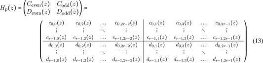
where Ceven(z), Codd(z), Deven(z), and Dodd(z) are r × r polynomial matrices (in z−1) that split C(z) and D(z) into two phases, such that
This architecture is illustrated in Figure 1 and leads to the same approximation coefficients aℓ and detail coefficients bℓ as before, where we used double subscripts to anticipate a multiresolution structure with repeated down-sampling and filtering steps later on.
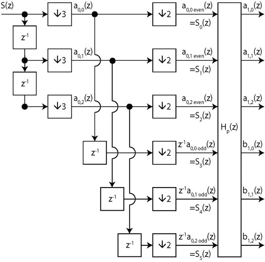
FIGURE 1. A single scale of a polyphase wavelet transform with r = 3 and a univariate input signal S(z) that is split into 2r phases, yielding r approximation components a1,ℓ and r detail components b1,ℓ.
For the 2r × 2r polyphase filter Hp(z) defined in Eq. 13 the orthogonality conditions of Eqs 3–5 translate into the equivalent condition:
This implies that Hp(z) is a lossless FIR filter, with coefficient matrices
Complementary to Eq. 13, which expresses Hp(z) in terms of C(z) and D(z), the low-pass and high-pass FIR filters C(z) and D(z) are reobtained from the polyphase filter Hp(z) by:
Parameterizing Lossless FIR Polyphase Filters
Lossless polyphase filters have a rich structure and have been well studied in the literature. See for instance [30, 31] for an accessible review of lossless filters and their key properties, including application areas and examples of the various uses they have. The basic property of a discrete-time lossless system, from which its name derives, is that the total energy of the output signals equals the total energy of the input signals, regardless of the signals being used. Here, energy is measured by the sum of squares of the values in the (discrete-time) signals. For Hp(z) this precise property is captured by Eq. 16. The point is that for |z| = 1 it holds that z−1 = z∗ (i.e., the complex conjugate) and since Hp(z) has real coefficients it follows that
For the construction of arbitrary lossless FIR polyphase filters (for given choices of r and n), the condition of Eq. 16 is not convenient to work with and impose directly. Equating coefficients for all the entries of the corresponding expressions on the left and on the right, can of course be done but does not provide orthogonality conditions in a form suitable for analytic or numerical computation. Instead, there is a body of literature which describes how the class of all 2r × 2r lossless systems of a fixed given order can be parameterized, by carrying out a recursion with respect to the system order, known as the tangential Schur algorithm; see [8]. This approach is flexible, as it allows the user to build in certain properties: for instance, by making specific choices for some parameters in the general procedure it allows one to parameterize the subclass of lossless FIR filters.
The following theorem was used in [27, 28] to parameterize (real) lossless FIR polyphase filters of a given order; see also [10, 31] for a similar yet slightly different construction. Here, the order k of a lossless FIR polyphase filter G(k)(z) is the McMillan degree of this rational matrix. For lossless functions this equals the degree of the denominator of the rational function det(G(k)(z)). For the lossless FIR polyphase filter Hp(z), the order n − 1 traditionally is the maximum lag of the filter, which relates to the length of the interval on which the multiwavelet lives. In the scalar case r = 1 these definitions coincide. In the multiwavelet case r ≥ 2 they do not. Generically, the McMillan degree and the maximum lag are the same for the lossless FIR polyphase filters in our class, but for special choices of the unit vectors uk they may be different: the maximum lag of Hp(z) is less than its McMillan degree n − 1 if and only if
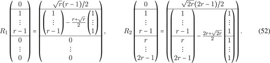
Theorem 3.1. Let G(k)(z) be a real 2r × 2r lossless FIR polyphase filter of order k ≥ 1. Then there exists a real 2r × 1 vector uk of norm ‖uk‖ = 1 such that G(k)(z) can be factored as:
where G(k−1)(z) is a real 2r × 2r lossless FIR polyphase filter of order k − 1.
This theorem shows that a lossless FIR polyphase filter of order k can be reduced in k iteration steps to a lossless FIR polyphase filter G(0)(z) of order 0, which is nothing else than a constant orthogonal matrix. We therefore drop the variable z for this last filter and simply write G(0).
For the polyphase matrix Hp(z) of the filter bank, the recursion makes clear that G(0) is in fact equal to the value of Hp(z) at z = 1: G(0) = Hp(1). This will make it more convenient to build in balanced vanishing moments than for the construction described in [10]. Generically, there will exist unit vectors u1, …, un−1 which allow Hp(z) to be factored as:
To make the parameterization explicit, all the vectors uk of norm 1 as well as the orthogonal matrix G(0) still can be parameterized in terms of scalar parameters. This is easily achieved. A 2r × 1 unit vector uk can be recursively parameterized as
The Balancing Problem
When processing a signal with a multiwavelet filter bank, the differences in spectral behavior of the r components of the multiscaling function may result in unbalanced channels of the low-pass filter. The consequences will further escalate in a multiresolution structure, when the filter bank is repeatedly applied to part of the output (the approximation signals) of a previous filtering step. The imbalance will adversely affect performance in compression and detection applications in signal and image processing, due to the fact that high and low frequencies start to mix. This problem is known as the balancing problem and was pointed out and characterized in detail in [9, 12, 24, 32].
The balancing problem is first encountered when processing a single scale of a multiwavelet filter bank with a sampled univariate signal as in Figure 1. Assume that the sampled input signal with z-transform S(z) is constant, then all down-sampled signals with z-transforms Sk(z) will be constant too and in fact be equal. A constant signal is supposed to pass unaltered through the polyphase filter, as the multiwavelet function Ψ(t) should pick up details and the multiscaling function Φ(t) the trend (an approximation to the signal); indeed, a constant function is all about trends and has no details. This can be achieved by imposing a zero-order vanishing moment on the filter bank, as is commonly done. This is the multiwavelet counterpart to the admissibility condition for scalar wavelets:
However, though each of the low-pass outputs a1,ℓ(z) will then be constant (due to the vanishing moment), their values may differ between components, since the vanishing moment by itself does not enforce coherence between the low-pass output channels. The signals a1,ℓ can therefore no longer be considered as phases from the constant approximation signal a(t). Though in itself this is already undesired as it hampers interpretation of the decomposition by the filter, this is further complicated when the signals are reused unaltered in a multiresolution structure. Spurious frequencies will then be introduced and severely compromise the usefulness and interpretability of the multiwavelet analysis. If a reconstruction of the approximation signal a(t) is done, possibly involving a number of upsampling and inverse filter steps, then this imbalance could be undone after which the signal can be split in 2r phases again as in Figure 1 for each wavelet scale. But to ensure that the filters will work properly on dyadic halfbands, this will involve extra effort whereas the interpretability of the approximation signals remains unfixed.
From a practical perspective, the approach as illustrated in Figure 2 is more appealing. Here, intermediate reconstruction and phase splitting between the scales is omitted. The approximation coefficient sequences are directly split into two phases and propagated to the next scale, as is common for scalar wavelets and consistent with the signal processing formulas (10)–(11). Without balancing, the consequence of this setup is that for a constant input signal at scale 2 the low-pass output a2,ℓ will no longer even be constant. This happens despite the fact that the zero-order vanishing moment ensures that constant signals are retained in the approximation low-pass output. With balancing, a constant input signal produces equal output signals a1,ℓ which remain well-behaved when further propagated to the next scale.
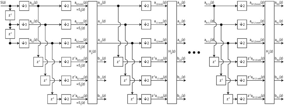
FIGURE 2. Multiresolution structure of a multiwavelet filter bank with r = 3 on a univariate input signal S(z) and N wavelet scales.
This issue generalizes to higher order vanishing moments which aim to have all polynomials up to a given degree in the approximation spaces. Including balanced vanishing moments of each order
The p-th order vanishing moment condition on the multiwavelet function Ψ(t) is given by:
It makes clear that polynomials of degree
Constructing specific orthogonal multiscaling functions which obey both (20) and (21) up to a given order p can be straightforward, e.g. by using a concatenation of r shifted versions of a Daubechies-p scaling function, where each ϕ[j](t) has been shifted by − j/r. Then, due to orthogonality of the shifted Daubechies scaling functions, clearly an orthogonal multiscaling function is obtained, which mimics the scalar setup entirely by having the wavelet forms ψ[j](t) now capture what is normally achieved by integer translations of a single wavelet. Using such Daubechies-p wavelets ensures vanishing moments up to and including order p − 1. Since each component ϕ[j](t) of the multiscaling function is just a time-shifted version of the others, it is also balanced.
However, constructing non-trivial orthogonal multiwavelet functions with different (non-shifted) wave forms and balanced vanishing moments up to a given order p is not straightforward. To address this question, we proceed as follows. (1) First, we derive vanishing moment conditions on the polyphase filter Hp(z). (2) Next, we derive additional balancing conditions. (3) We investigate how to satisfy all these conditions, up to a chosen order p, by building them into the parameterization of lossless FIR polyphase filters of order n. This is achieved for orders 0 and 1, whereas for order 2 the conditions can be brought into a form which can be used for numerical search.
Vanishing Moment Conditions for Multiwavelets
Let us introduce the r × 1 vectors vk and wk (for k = 0, 1, 2, …) by defining:
These are the k-th moments of the multiscaling and multiwavelet functions. From the dilation and wavelet Eqs 1–2, we derive the following relationships. First, integration gives
Here it is used that
Next, if we first multiply left and right hand sides of the dilation and wavelet equations by t and then integrate, we obtain in a similar fashion:
Here it is used that
More generally, if we first multiply left and right hand sides of the dilation and wavelet equations by t2 and then integrate, we obtain:
Here we wrote
The vanishing moment conditions up to and including order p are:
because wk represents the (vector) wavelet coefficient of the polynomial signal tk for the untranslated multiwavelet Ψ(t), and these wavelet coefficients should all vanish. The vanishing moment conditions state that the filter coefficients Ck and Dk (k = 0, 1, …, 2n − 1) should be such as to allow these equations to be satisfied for some vectors v0, v1, …, vp, representing the moments of the multiscaling function.
For orders p = 0, p = 1, and p = 2, the vanishing moment conditions above can be rewritten in terms of the filters C(z) and D(z). Focusing on the equations involving C(z) (the other equations with D(z) are handled entirely analogously) we see from differentiation, that
whence
The relationship (17) links the filters C(z) and D(z) to the polyphase filter Hp(z). Differentiation after multiplication by any constant vector v gives:
which produces at z = 1:
An additional differentiation step yields:
which gives at z = 1:
These results are combined and summarized in the following theorem.
Theorem 3.2. Let the vectors vk (k = 0, 1, 2) be defined as in Eq. 22. The polyphase filter Hp(z) imposes a vanishing moment of order 0 on the multiwavelet if it holds that:
A vanishing moment of order 1 occurs if:
A vanishing moment of order 2 occurs if:
To have balanced vanishing moments of order up to and including p, requires extra conditions on the vectors vk, k = 0, 1, 2, …, p. This is addressed next.
Balanced Vanishing Moment Conditions for Multiwavelets
The balancing conditions can be computed from Eq. 21 by integration.
For order p = 0 this gives that all entries of v0 are equal, say with value α0. To find α0, the cascade algorithm is useful. For the Haar multiwavelet in the initialisation step, the scaling function ϕ[j](t) is positive and constant on the interval
For order p = 1 it is obtained that
By inspecting what happens for balanced orthogonal multiwavelets generated from scalar orthogonal wavelets with vanishing moments through shifting, just as explained earlier for the Haar multiwavelet, we find that the value of λ varies between multiwavelets. It therefore is left as a free parameter.
Next, for order p = 2 it is obtained that
The parameter μ is again left free.
From a signal processing point of view, if a signal s(t) is a polynomial in t of degree
These additional balancing conditions on the vectors v0, v1 and v2 can now be combined with the previous vanishing moment conditions. This gives the following result.
Theorem 3.3. (a) The polyphase filter Hp(z) imposes a balanced vanishing moment of order 0 on the multiwavelet structure if it holds that:
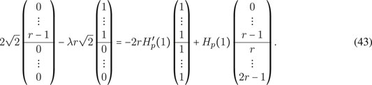
(b) Balanced vanishing moments of orders 0 and 1 occur if in addition to the condition of (a) it holds that there exists a constant λ such that:
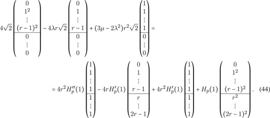
(c) Balanced vanishing moments of orders 0, 1 and 2 occur if in addition to the conditions of (a) and (b) it holds that there exists a constant μ such that:
The proof of this result is by direct computation, using Eqs 39–41 together with Thm. 3.2. Part (a) of this theorem was shown earlier in the work of [9] and used before in [27]. Parts (b) and (c) are novel characterizations, using the lossless polyphase filter and its derivatives at z = 1.
Parameterization of Lossless FIR Polyphase Filters With a Balanced Vanishing Moment of Order 0
A parametrization of lossless FIR polyphase filters with a balanced vanishing moment of order 0 has previously been described in [27, 28]. We present it here for completeness and also because some of the techniques and notation will be reused when we address balancing of order 1. In fact, the parameterization in Eq. 19 is slightly different from the parameterization used in the literature cited above, but the basic ideas are similar.
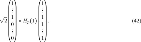
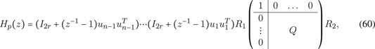
From part (a) of Thm. 3.3 we have that for a zero-order balanced vanishing moment, the orthogonal matrix Hp(1) must map the vector
Clearly
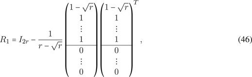
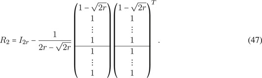
Note that the zero-order condition can be rewritten as
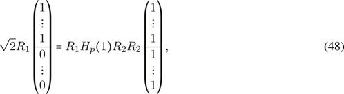
and in this way turns into
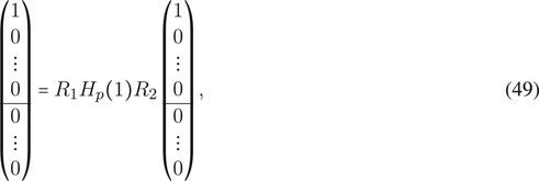
The matrix R1Hp(1)R2 is again orthogonal, and it therefore necessarily is of the form
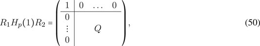
with Q an orthogonal matrix of size (2r − 1) × (2r − 1). The converse clearly also holds true, which motivates the following result.
Theorem 3.4. All lossless FIR polyphase filters Hp(z) of order n − 1 with a balanced vanishing moment of order 0 are obtained as:
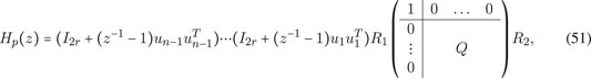
where R1 and R2 are the fixed Householder matrices given in Eqs 46, 47, where Q ranges over the set of (2r − 1) × (2r − 1) orthogonal matrices, and where u1, u2, …, un−1 ranges over the set of n − 1 unit vectors of size 2r × 1.
Explicit parameterization of the orthogonal matrix Q can be done with Givens rotations and Householder matrices as indicated earlier, see Section 2.2. There we also showed how a parameterization of the unit vectors u1, …, un−1 can be obtained. We see that manipulating the vectors uk (or increasing their number) does not affect the zero order balancing property as it is fully implied by the structure of Eq. 51. This is conveniently exploited when considering an additional balanced vanishing moment of order 1 below.
Parameterization of Lossless FIR Polyphase Filters With Balanced Vanishing Moments of Orders 0 and 1
To build an extra balanced vanishing moment of order 1 into the lossless FIR polyphase filters Hp(z), retaining the balanced vanishing moment of order 0, the idea is to start from the parameterization in Thm. 3.4 and to refine the structure of the orthogonal matrix Q and the unit vectors u1, …, un−1 to meet the condition of Eq. 43. The latter condition involves an additional scalar parameter λ, which can be freed up by premultiplication of all the terms in the equation by the Householder matrix R1 of Eq. 46 as we will now show. In view of the structure of Hp(1) = G(0) given by Eq. 50, it is useful to first work out the following two matrix-vector products (the horizontal lines are just for clarity):
The matrix
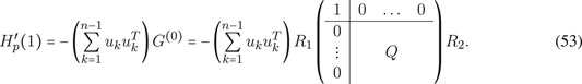
Using all of this, condition (43) takes the form:
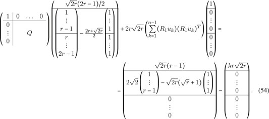
The parameter λ only appears in the top row of this vector equation. Selecting this row admits computation of λ as:
Here,
for some scalar θk ∈ [0, π] and with
whereas, upon division by
Introducing the following (r − 1) × 1 vectors hr, for positive integers r:
allows us to summarize these findings concisely in the following theorem.
Theorem 3.5. All lossless FIR polyphase filters Hp(z) of order n − 1 with two balanced vanishing moments, of orders 0 and 1, are obtained as:
where R1 and R2 are the fixed Householder matrices given in Eqs 46, 47, where Q is (2r − 1) × (2r − 1) orthogonal, and where uk (k = 1, …, n − 1) are unit vectors of size 2r × 1 parameterized as
with scalar θk ∈ [0, π], unit vectors
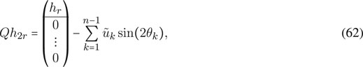
with the vectors hr and h2r defined as in Eq. 59.
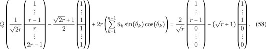
To complete the parameterization of Theorem 3.5, we now show how all tuples of orthogonal Q, unit vectors
For hr it is straightforward to compute its norm ‖hr‖ as
For r = 1, we encounter the scalar orthogonal wavelet case, and the vector hr is in fact empty (of size 0, ×, 1). Balancing is not meaningful then. Indeed the condition reduces to the scalar equation
Focusing on the multiwavelet case with r ≥ 2, it is noted that ‖hr‖ increases monotonically from
Writing
The idea of the parameterization, is to build the vectors gk one by one, such that the condition remains feasible, i.e., the remaining vectors-to-be-constructed can still be assigned values to meet Eq. 62. Suppose g1, …, gℓ−1 have been chosen and denote (for ℓ = 1, 2, …, n):
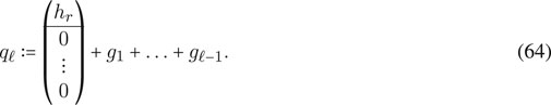
Then, for ℓ = 1, 2, …, n − 2, the vector gℓ must be chosen such that the vector qℓ+1 = qℓ + gℓ is in (or on) the hyperball (centered at the origin) of radius
This still allows the right-hand side of Eq. 62, viz. the expression qℓ+1 + gℓ+1 + ⋯ + gn−1 = qn, to eventually land on the hypersphere of vectors with norm ‖h2r‖. For the left-hand side expression Qh2r, note that the norm equals ‖h2r‖ for every orthogonal Q, and that a suitable orthogonal matrix Q can always be constructed to make Qh2r equal to that landing point (a Householder matrix would do). In fact, all such orthogonal Q can be constructed along the same lines as before when constructing G(0) for balancing of order 0, as we will demonstrate below in Eq. 74. Note that if one cannot land on that hypersphere the construction is infeasible, since the norm of Qh2r is fixed; so this precisely characterizes feasibility. (Note, also, that points inside the hypersphere of radius ‖h2r‖ can always be brought to a point on the hypersphere in one step, by adding a single vector gk, since ‖h2r‖ < 1; therefore one need not consider a constraint on the inside of the hypersphere.)
For ℓ = 1, 2, …, n − 2, we proceed as follows. If ‖qℓ‖ ≤ rℓ − 1, then gℓ can be any vector of norm
If ‖qℓ‖ > rℓ − 1, then let
with scalar coefficients αℓ (still unrestricted) and βℓ ≥ 0. For gℓ to be feasible it must hold that: (1) ‖gℓ‖ ≤ 1, (2) ‖qℓ + gℓ‖ ≤ rℓ. Because qℓ and
Once αℓ is chosen, βℓ can be chosen non-negative but such that the two conditions remain satisfied. This gives:
For ℓ = n − 1, choosing the final vector gn−1 (of norm
If ‖qn−1‖ ≤ 1 − rn−1, then qn can land on every point of the hypersphere with radius rn−1 by choosing gn−1 as the difference between that point and qn−1.
If ‖qn−1‖ > 1 − rn−1, then the hypersphere centered at the origin with radius rn−1 and the hypersphere centered at qn−1 with radius 1 intersect at points
Subtracting the first equation from the second leaves a linear equation for αn−1, which gives:
This determines the minimal value for αn−1 to give solutions on the hypersphere for qn. The maximal value for αn−1 is obtained with βn−1 = 0 and equals
and
Finally, to find all feasible orthogonal Q once the right-hand side expression qn is constructed to have ‖qn‖ = rn−1 = ‖h2r‖, let R3 be the Householder matrix which maps qn to
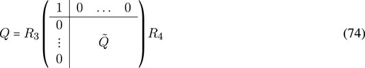
with
Balanced Vanishing Moments of Orders 0, 1 and 2
Incorporating an additional balanced vanishing moment of order p = 2, requires further refinement of the current parameterization such that condition (44) is also satisfied. As we have not developed a way to incorporate this into a parameterization, we will only show how the condition can be reworked into a form which makes it suitable to be added as a constraint to the parametrization in terms of the parameters used before.
A first step to achieve this, is to free up and remove the parameter μ by premultiplication of all terms in the condition by the Householder matrix R1. The effect of this is that μ only appears in the term
The actual conditions for balancing of order 2, are then captured by the remaining 2r − 1 equations in which μ no longer appears. The parameter λ which does show up in them, should be replaced by its value in terms of the chosen parameters as given in Eq. 57. This gives the constraints in a form which can readily be used for numerical optimization, using a routine for constrained optimization which admits nonlinear constraints.
Design Criteria for Matching
For the scalar orthogonal wavelet design case, sparsity of a prototype signal was already advocated in [7]. This is appealing for detection and compression purposes. There it was also shown that maximization of sparsity of the vector of all approximation and detail coefficients w = {wk} in the setting with a critically sampled orthogonal wavelet transform, boils down to either: 1) maximization of the variance of the sequence of absolute values |wk| of the coefficients, or 2) maximization of the variance of the squared wavelet coefficients. This is due to the fact that Parseval’s identity holds [4], which makes that the sum of squares of all the wavelet and detail coefficients equals the sum of squares of all the values of the digital signal being processed. This result does obviously not change for orthogonal multiwavelet design. Hence [[7], Theorem 1], holds in the current setting too:
Theorem 3.6. Let w be the vector of the approximation coefficients at the coarsest scale and the detail coefficients at all scales, resulting from the processing of a signal s by means of an orthogonal multiwavelet filter bank across multiple scales. Then:
1) Maximization of the variance of the vector of absolute values {|wk|} is equivalent to minimization of the L1-norm of the vector w.
2) Maximization of the variance of the energy vector {|wk|2} is equivalent to maximization of the L4-norm of the vector w.
For practical applications the latter criterion, L4-maximization, is more appealing than the former since it can be combined with weighing both in scale and location [27]. This allows for designing a matched multiwavelet, where each of the components of Φ(t) is forced to focus on a single aspect in a signal (see Section 3.2 for an example).
If instead of a critically sampled multiwavelet transform an undecimated multiwavelet transform [33] is used, this has advantages for detection purposes, since due to the redundant representation time-invariance is achieved. The lack of down-sampling, however, causes an abundance of coefficients at coarser scales. To preserve conservation of energy properties for orthogonal multiwavelets, this abundance can be counteracted by dyadic discounting of energies towards coarser scales as in [7]. This makes it possible to use adapted versions of the L1-minimization and L4-maximization criteria for undecimated multiwavelet transforms promoting sparsity.
Another criterion one might consider is entropy. One can quantify the effectiveness of compression algorithms in terms of entropy [34]. As suggested in [35], entropy can be used to select an orthogonal wavelet basis, and a similar approach can serve as a design criterion. This is certainly appealing for compression purposes.
Illustrative Examples
Experiment to Illustrate the Balancing Problem
The effects of having unbalanced vanishing moments are easily illustrated by considering what happens if a constant signal is fed into an unbalanced orthogonal multiwavelet filter bank with multiplicity r = 2 and of order n − 1 = 3, using the construction scheme in Theorem 3.1, but without balancing. To this end we took Q = I2r−1 = I3 and we changed the Householder matrix R1 to produce a non-constant vector v0.
When a constant input signal is fed into an orthogonal multiwavelet filter bank with an order 0 unbalanced vanishing moment, as described in Section 3.1, the results (depending on the exact choice of coefficients) are as shown in Figure 3. What can be observed in the top figure, is that the detail coefficients are all zero for both channels (consistent with the imposed vanishing moments), and the approximation coefficients are constant per channel, but the values are different between the channels. In terms of the notation in Eqs 8, 9, the detail vector coefficients bk are all zero, the approximation vector coefficients ak are all constant, but their entries
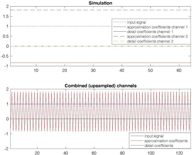
FIGURE 3. Top: result of feeding a constant signal into an unbalanced multiwavelet filter bank. Bottom: Consequence of interpreting the output of the two low-pass channels as phases of a signal.
In the bottom figure of Figure 3 it is displayed what the resulting signal looks like if the outputs are nevertheless interpreted as the two phases of a signal.
If the outputs are now processed further with the multiwavelet filter bank for a few more scales, this has the effect that at later scales the constant nature of the original signal is lost and the detail coefficients become nonzero, as demonstrated in Figure 4.
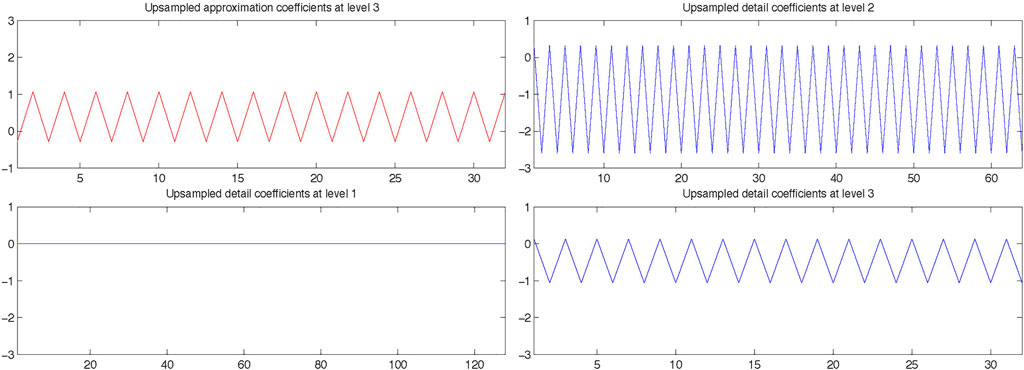
FIGURE 4. Result of processing a constant signal with an unbalanced orthogonal multiwavelet filter bank with a vanishing moment of order 0 for three scales.
Example of Multiwavelet Design for ECG Feature Detection
In this section we introduce an example for balanced multiwavelet design. We will employ L4-maximization with weighted masking to match the multiwavelet filter bank to a prototype signal. The example evolves around creating a representation for a prototype ECG signal as is commonly encountered in the field of cardiology. The goal of this design is for feature detection to distinguish and detect different complexes in the ECG signal.
Feature detection is an application that makes efficient use of the different components of the multiwavelet. The idea of feature detection via multiwavelets is to design each component of the multiwavelet to detect a specific feature in the signal. Orthogonality between the components of the scaling- and wavelet function allows the multiwavelet to detect up to r orthogonal features, which cannot all be accurately detected by a scalar wavelet at the same time. Since features in a signal need not be orthogonal but can be overlapping, making them hard to separate, the multiwavelet approach is fundamentally different from template based approaches. When training orthogonal multiwavelets on different features, the goal is to have them pick up orthogonal aspects from the features that help to distinguish between them.
For this application the variance maximizing L4-objective function is no longer measured across all the wavelet coefficients. Instead, a time-scale mask is employed for each component of the multiwavelet [28], and the value of the objective function of a component is only measured on the wavelet coefficients that are in the time-scale mask. In this way, maximization of the criterion forces energy into the masked areas, helping the multiwavelets to focus on the user-selected signal features covered by the time-scale masks. (This same idea is less conveniently pursued with L1-minimization, because minimization will force energy out of the masked areas, but while the energy leaks away this does not mean that useful multiwavelets are promoted.)
In this example, the design procedure employs a first-order balanced orthogonal multiwavelet, with focus on the approximation coefficients rather than the detail coefficients, and aiming to detect features by looking at the peaks of the approximation coefficients at masked areas at the coarsest scale l = 3.
It can be seen from Figure 5 that the first scaling function mainly represents the QRS-complex on which it was trained, whereas the second scaling function manages to capture the T-wave on which it was trained. By thresholding the approximation coefficients of the first channel the location of the QRS-complex can be obtained. By thresholding the second channel the location of the T-peak is obtained. Both channels can detect the feature that they were designed for independently from one another. This is remarkable, as the T-wave overlaps in spectrum and waveform with the QRS-complex, which carries far more energy. Though the second wavelet also picks up some energy from the QRS-complex, it still allows to detect the T-peak location with simple thresholding. This demonstrates that a matched multiwavelet is a powerful signal processing tool to detect and discriminate between different features in a signal.
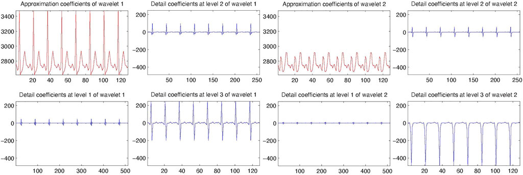
FIGURE 5. Result of designing a multiwavelet with r = 2 for feature detection in the prototype ECG signal. Shown for each wavelet are the values of the approximation coefficients at the coarsest scale, and of the detail coefficients for three increasing scales (from fine to coarse). The first wavelet was trained on the QRS-complex, the second wavelet on the T-wave in the ECG signal.
Example of an Orthogonal Multiwavelet With Compact Support, Multiplicity 3 and Balanced Vanishing Moments of Orders 0, 1, and 2
In this example we show an orthogonal multiwavelet filter with multiplicity r = 3, involving a lossless FIR polyphase filter Hp(z) of order n − 1 = 3, with balanced vanishing moments of orders p = 0, p = 1, and p = 2 as a concrete example of multiwavelet design with three balanced vanishing moments. To obtain such a filter, we utilized the parameterization that was introduced in Section 2.7 for multiwavelets with balanced vanishing moments of orders 0 and 1, and we followed the approach of Section 2.8. For r = 3 and n − 1 = 3, we first chose random parameters to obtain an initial orthogonal multiwavelet only lacking a second order vanishing moment. From there, constrained optimization was used to adapt the parameters to satisfy condition (44), producing an orthogonal multiwavelet with three balanced vanishing moments.
For this example, the FIR polyphase filter Hp(z) = H0 + H1z−1 + H2z−2 + H3z−3 has the following coefficient matrices Hk:
Associated with this polyphase filter are the wavelet and scaling functions as shown in Figure 6.
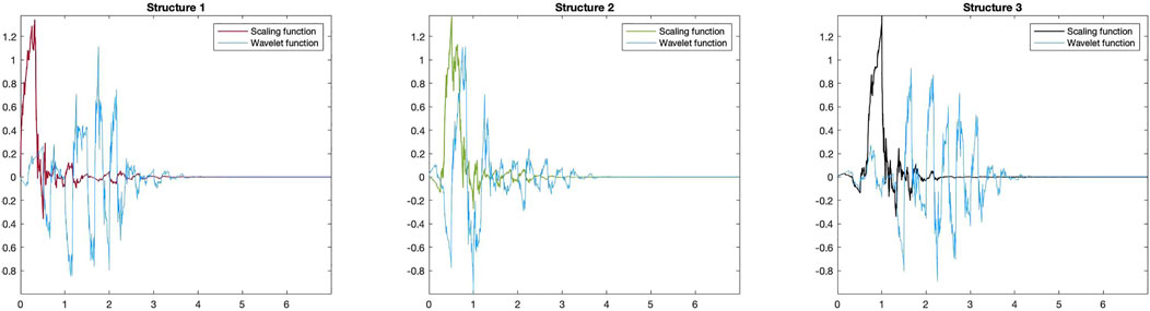
FIGURE 6. Wavelet and scaling functions obtained from the polyphase filter in Section 3.3.
By definition, the Householder matrices R1 and R2 are given by:
For the example, the orthogonal matrix Q and the unit vectors u1, u2 and u3 which appear in the parameterization of Hp(z) have the following values:
The values of the parameters λ and μ encountered for this particular balanced multiwavelet of order 2, are given by:
The resulting unit vectors R1u1, R1u2, and R1u3 are:
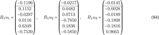
These vectors R1uk (k = 1, 2, 3) are partitioned as
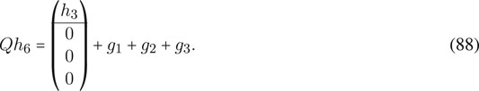
The vectors gk, which feature in the parameterization for balancing of order 1, are defined as
The vectors h3 and h6 are defined as follows:
having norms:
It is verified by direct computation upon substitution into Eqs 16, 51, 42, 43, 44, 62 that the orthogonality conditions as well as the three balanced vanishing moment conditions for order p = 0, 1, 2 are all properly satisfied, and entirely consistent with the proposed parameterization.
Discussion
The results in Section 3.1 show, from a signal processing perspective, the importance of having balanced vanishing moments for multiwavelets. Not having this means that polynomials do not yield zero detail coefficients in subsequent scales, even if the required vanishing moments are built in. The example in Section 3.2 shows that if the available remaining freedom is used to promote sparsity, this has a benefit for detection purposes. Other design objectives could also be employed. When employing weighing over scales, this also opens the opportunity to use overcomplete representations for shift-invariance. Masking in the time-scale plane allows to focus on selected parts of a prototype signal. When one would switch to a criterion based on the information value, this can be valuable for compression purposes.
In Section 3.3 a concrete example was worked out for the design of orthogonal multiwavelets with compact support and three balanced vanishing moments (orders 0, 1, and 2) and multiplicity r = 3. Previous examples of orthogonal multiwavelets in the literature with several balanced vanishing moments either had balancing only up to order 1, or multiplicity r = 2; see [9, 11]. The Gröbner basis approach used there is a limiting factor for finding matching balanced multiwavelets to applications, because the approach does not allow for excess degrees of freedom. In this paper we advocated a different approach by building an explicit parameterization which allows free parameters to be tuned for various purposes. We have shown how all balanced orthogonal multiwavelets of orders 0 and 1 can be obtained for arbitrary multiplicity r and any given polyphase filter order (McMillan degree), which we consider a major step forward in making multiwavelets applicable.
Data Availability Statement
The original contributions presented in the study are included in the article/Supplementary Material, further inquiries can be directed to the corresponding author.
Author Contributions
JK, SS, and RP together conceived and explored the concept of parameterizing balanced orthogonal multiwavelets with built-in vanishing moment properties. Numerical simulations were implemented and performed by SS. JK, and RP provided the background on multiwavelets, balancing, and parameterisation of lossless systems, and provided cardiac signal data. JK and RP composed the final article based on an initial draft by SS.
Conflict of Interest
The authors declare that the research was conducted in the absence of any commercial or financial relationships that could be construed as a potential conflict of interest.
Publisher’s Note
All claims expressed in this article are solely those of the authors and do not necessarily represent those of their affiliated organizations, or those of the publisher, the editors and the reviewers. Any product that may be evaluated in this article, or claim that may be made by its manufacturer, is not guaranteed or endorsed by the publisher.
Footnotes
1In those papers, p-order balancing is defined to correspond to p balanced vanishing moments, of orders 0, 1, …, p − 1. In this paper we will call this ‘balanced up to order p − 1.’
2Note that, unlike what is common in most of the literature, we have chosen in our definition of the dilation and wavelet equation above to use functions Φ(2t + k) rather than Φ(2t − k), in line with the convention in [7]. This causes no loss of generality, but makes that the multiscaling and multiwavelet functions in Φ(t) and Ψ(t) are all compactly supported on the negative interval (−(2n − 1), 0] as can be quickly derived from (1) and (2). This has the two-fold advantage that we can save on the notation and the number of filters required in the rest of this work, as well as that we can work with causal filters and avoid unnecessary delay or advance operators when switching to a signal processing perspective. Should one switch to using functions Φ(2t − k) on the right-hand side of the dilation and wavelet equations, then the time-reversed functions Φ( − t) and Ψ( − t) are the new solutions in the adapted setting.
3The convolution sums in Eqs 10–11, involving s2ℓ−k rather than s2ℓ+k, appear because of the convention we adopted for the dilation and wavelet equation.
4To compute the McMillan degree of a lossless FIR polyphase filter
5Givens rotations and Householder reflections are commonly used to perform QR-decomposition. When applied to an orthogonal matrix, the upper triangular R is in fact diagonal with all entries on its main diagonal equal to ± 1. The space of orthogonal matrices has two connected components, characterized by the sign of the determinant ± 1, which is something to take into account when parameterizing this space. Givens rotations all have determinant 1 and are used to create zeros one by one; they involve a single angular parameter. Householder reflections all have determinant − 1 and are used to create multiple zeros at once; they involve a vector of norm 1 requiring multiple angular parameters. See [37]. We will introduce Householder matrices in Eq. 45.
6To parameterize all such
References
1. Grossmann, A, and Morlet, J. Decomposition of Hardy Functions into Square Integrable Wavelets of Constant Shape. SIAM J Math Anal (1984) 15:723–36. doi:10.1137/0515056
2. Grossmann, A. Wavelet Transforms and Edge Detection. In: S Albeverio, P Blanchard, M Hazewinkel, and L Streit, editors. Stochastic Processes in Physics an Engineering. Dordrecht, The Netherlands: D. Reidel Publishing Company (1988). p. 149–57. ISBN: 90-277-2659-0. doi:10.1007/978-94-009-2893-0_7
3. Daubechies, I. Orthonormal Bases of Compactly Supported Wavelets. Comm Pure Appl Math (1988) 41:909–96. doi:10.1002/cpa.3160410705
4. Mallat, S. A Wavelet Tour of Signal Processing: The Sparse Way. Amsterdam: Academic Press (2009). doi:10.1016/B978-0-12-374370-1.X0001-8
5. Karel, JMH, Peeters, RLM, Westra, RL, Moermans, KMS, Haddad, SAP, and Serdijn, WA. Optimal Discrete Wavelet Design for Cardiac Signal Processing. In: Proceeding: 27th Annual International Conference of the IEEE Engineering in Medicine and Biology Society. IEEE Engineering in Medicine and Biology Society (EMBC 2005); 1-4 September, 2005; Shanghai, China. IEEE (2005). p. 2769–72. doi:10.1109/IEMBS.2005.1617046
6. Peeters, R, and Karel, J. Data Driven Design of an Orthogonal Wavelet with Vanishing Moments. In: 21st International Symposium on Mathematical Theory of Networks and Systems; Groningen, Netherlands, 2014 7–11 July (2014). p. 1665–72.
7. Karel, J, and Peeters, R. Orthogonal Matched Wavelets with Vanishing Moments: A Sparsity Design Approach. Circuits Syst Signal Process (2018) 37:3487–514. doi:10.1007/s00034-017-0716-1
8. Hanzon, B, Olivi, M, and Peeters, RLM. Balanced Realizations of Discrete-Time Stable All-Pass Systems and the Tangential Schur Algorithm. Linear Algebra Appl (2006) 418:793–820. doi:10.1016/j.laa.2006.03.027
9. Lebrun, J, and Vetterli, M. High-order Balanced Multiwavelets: Theory, Factorization, and Design. IEEE Trans Signal Process (2001) 49:1918–30. doi:10.1109/78.942621
10. Strang, G, and Nguyen, T. Wavelets and Filter Banks. Wellesley, MA.: Wellesley-Cambridge Press (1996). ISBN: 978-0961408879.
11. Selesnick, IW. Multiwavelet Bases with Extra Approximation Properties. IEEE Trans Signal Process (1998) 46:2898–908. doi:10.1109/78.726804
12. Chui, CK, and Jiang, Q. Balanced Multi-Wavelets in $\mathbb R^s$. Math Comp (2004) 74:1323–45. doi:10.1090/S0025-5718-04-01681-3
13. Sun, H, Zi, Y, and He, Z. Wind Turbine Fault Detection Using Multiwavelet Denoising with the Data-Driven Block Threshold. Appl Acoust (2014) 77:122–9. doi:10.1016/j.apacoust.2013.04.016
14. Chen, J, Li, Z, Pan, J, Chen, G, Zi, Y, Yuan, J, et al. Wavelet Transform Based on Inner Product in Fault Diagnosis of Rotating Machinery: A Review. Mech Syst Signal Process (2016) 70-71:1–35. doi:10.1016/j.ymssp.2015.08.023
15. Chen, J, Wan, Z, Pan, J, Zi, Y, Wang, Y, Chen, B, et al. Customized Maximal-Overlap Multiwavelet Denoising with Data-Driven Group Threshold for Condition Monitoring of Rolling Mill Drivetrain. Mech Syst Signal Process (2016) 68-69:44–67. doi:10.1016/j.ymssp.2015.07.022
16. Hong, L, Liu, X, and Zuo, H. Compound Faults Diagnosis Based on Customized Balanced Multiwavelets and Adaptive Maximum Correlated Kurtosis Deconvolution. Measurement (2019) 146:87–100. doi:10.1016/j.measurement.2019.06.022
17. He, J, Yang, Z, Chen, C, Li, G, Li, Z, and Jia, Y. Improved Multiwavelet Denoising with Neighboring Coefficients of Cutting Force for Application in the Load Spectrum of Computer Numerical Control Lathe. Adv Mech Eng (2018) 10:1–11. doi:10.1177/1687814018754674
18. Alkhidhr, H, and Jiang, Q. Correspondence between Multiwavelet Shrinkage and Nonlinear Diffusion. J Comput Appl Math (2021) 382:113074. doi:10.1016/j.cam.2020.113074
19. Jiang, Q. On the Design of Multifilter banks and Orthonormal Multiwavelet Bases. IEEE Trans Signal Process (1998) 46:3292–303. doi:10.1109/78.735304
20. Chui, CK, and Jiang, Q. Multivariate Balanced Vector-Valued Refinable Functions. In: W Haussmann, K Jetter, M Reimer, and J Stöckler, editors. Modern Developments in Multivariate Approximation. Springer Basel AG: Basel, Vol. 145 (2003). p. 71–102. doi:10.1007/978-3-0348-8067-1_4
21. Han, B, and Lu, R. Compactly Supported Quasi-Tight Multiframelets with High Balancing Orders and Compact Framelet Transforms. Appl Comput Harmonic Anal (2021) 51:295–332. doi:10.1016/j.acha.2020.11.005
22. Han, B, and Lu, R. Multivariate Quasi-Tight Framelets with High Balancing Orders Derived from Any Compactly Supported Refinable Vector Functions. Sci China Math (2021):1–30. [Epub ahead of print]. doi:10.1007/s11425-020-1786-9
23. Lebrun, J, and Vetterli, M. Balanced Multiwavelets. In: 1997 IEEE International Conference on Acoustics, Speech, and Signal Processing; 21-24 April, 1997; Munich, Germany, 3 (1997). p. 2473–6. doi:10.1109/ICASSP.1997.599579
24. Lebrun, J, and Vetterli, M. Balanced Multiwavelets Theory and Design. IEEE Trans Signal Process (1998) 46:1119–25. doi:10.1109/78.668561
25. Bacchelli, S, Cotronei, M, and Lazzaro, D. An Algebraic Construction of K-Balanced Multiwavelets via the Lifting Scheme. Numer Algorithms (2000) 23:329–56. doi:10.1023/A:1019120621646
26. Li, B, and Peng, L. Balanced Multiwavelets with Interpolatory Property. IEEE Trans Image Process (2011) 20:1450–7. doi:10.1109/TIP.2010.2092439
27. Peeters, RLM, Karel, JMH, Westra, RL, Haddad, SAP, and Serdijn, WA. Multiwavelet Design for Cardiac Signal Processing. In: Proceeding: 28th Annual International Conference of the IEEE Enigneering in Medicine and Biology Society (EMBC 2006); 30 August-3 September, 2006; New York City (2006). p. 1682–5. doi:10.1109/IEMBS.2006.259733
28. Karel, J. A Wavelet Approach to Cardiac Signal Processing for Low-Power Hardware Applications. Universitaire Pers Maastricht (2009). ISBN: 978-90-5278-887-6.
29. Smith, M, and Barnwell, T. A Procedure for Designing Exact Reconstruction Filter banks for Tree-Structured Subband Coders. IEEE Int Conf Acoust Speech Signal Process (1984) 9:421–4. doi:10.1109/ICASSP.1984.1172486
30. Vaidyanathan, P. Theory and Design of M-Channel Maximally Decimated Quadrature Mirror Filters with Arbitrary M, Having the Perfect-Reconstruction Property. IEEE Trans Acoust Speech Signal Process (1987) 35:476–92. doi:10.1109/TASSP.1987.1165155
31. Vaidyanathan, PP, and Doganata, Z. The Role of Lossless Systems in Modern Digital Signal Processing: a Tutorial. IEEE Trans Educ (1989) 32:181–97. doi:10.1109/13.34150
32. Selesnick, IW. Balanced Multiwavelet Bases Based on Symmetric FIR Filters. IEEE Trans Signal Process (2000) 48:184–91. doi:10.1109/78.815488
33. Nason, GP, and Silverman, BW. The Stationary Wavelet Transform and Some Statistical Applications. In: A Antoniadis, and G Oppenheim, editors. Lecture Notes in Statistics: Wavelets and Statistics. New York, NY: Springer-Verlag, Vol. 103 (1995). p. 281–99. doi:10.1007/978-1-4612-2544-7_17
34. Shannon, CE. A Mathematical Theory of Communication. Bell Syst Tech J (1948) 27:379–423. doi:10.1002/j.1538-7305.1948.tb01338.x
35. He, H, Tan, Y, and Wang, Y. Optimal Base Wavelet Selection for Ecg Noise Reduction Using a Comprehensive Entropy Criterion. Entropy (2015) 17:6093–109. doi:10.3390/e17096093
36. Peeters, R, Olivi, M, and Hanzon, B. Balanced Realization of Lossless Systems: Schur Parameters, Canonical Forms and Applications. In: Proceedings of the 15th IFAC SYSID 2009; 6-8 July, 2009; Saint-Malo (2009). p. 273–83. doi:10.3182/20090706-3-fr-2004.00045
Keywords: wavelet theory, orthogonal multiwavelets, balanced vanishing moments, matched wavelets, sparsity, parameterization, lossless polyphase filters
Citation: Karel JM, van Steenkiste S and Peeters RL (2022) The Design of Matched Balanced Orthogonal Multiwavelets. Front. Appl. Math. Stat. 7:785803. doi: 10.3389/fams.2021.785803
Received: 27 October 2021; Accepted: 24 November 2021;
Published: 20 January 2022.
Edited by:
Qingtang Jiang, University of Missouri–St. Louis, United StatesReviewed by:
Lihong Cui, Beijing University of Chemical Technology, ChinaRan Lu, Hohai University, China
Copyright © 2022 Karel, van Steenkiste and Peeters. This is an open-access article distributed under the terms of the Creative Commons Attribution License (CC BY). The use, distribution or reproduction in other forums is permitted, provided the original author(s) and the copyright owner(s) are credited and that the original publication in this journal is cited, in accordance with accepted academic practice. No use, distribution or reproduction is permitted which does not comply with these terms.
*Correspondence: Ralf L.M. Peeters, cmFsZi5wZWV0ZXJzQG1hYXN0cmljaHR1bml2ZXJzaXR5Lm5s