Experimental and Numerical Studies on the Focused Waves Generated by Double Wave Groups

Introduction

Given the future of conventional energy sources, there is a great need to establish sustainable energy systems for substitution (Cruz, 2008). Currently, ocean wave energy, as a large, widespread, and environmental renewable resource, is in the spotlight with large potential and consequently more and more wave energy devices come into being (Tunde and Hua, 2018). Generally, the higher the wave height is, the greater the ocean wave energy that can be converted. However, extreme waves (freak waves or rogue waves), which possess the characteristic of large wave heights and strong non-linearity, often exceed the endurance limit of wave energy devices and cause huge damage to these devices as well as serious loss of life and property (Kharif and Pelinovsky, 2003; Toffoli et al., 2005; Bitner-Gregersen and Toffoli, 2014). In recent years, as human activities (such as the exploration and development of marine resources) move toward the deep ocean and become frequent, the chance to encounter freak waves increases. How to avoid the damage caused by extreme waves is one issue that must be faced in the process of promoting the development of ocean wave energy. Thus, study on the freak wave generation is of great practical significance, and it should attract more and more attention.

Freak waves are universal in real sea states and have been observed under various circumstances. To understand the complex phenomenon, associated research has been conducted on the physical mechanisms of freak wave generation, which can be categorized into two types: linear and non-linear mechanisms (Kharif and Pelinovsky, 2003; Dysthe et al., 2008; Adcock and Taylor, 2014). Early studies on the generation of freak waves focused on the linear mechanism, in which the wavefield can be considered as the sum of a large number of independent monochromatic waves with different frequencies and directions of propagation. The dispersion of the waves, the refraction effect of the terrain, the modulation of the current field, and the interaction of waves propagating in different directions can also lead to the generation of freak waves (Kharif and Pelinovsky, 2003). Many researchers have adjusted the initial phase of each wave component and used linear superposition to focus at a specified location and time to form freak waves (Zhao et al., 2009, 2020; Li and Liu, 2015). Although the linear mechanism can directly explain the generation of freak waves, the assumption of linearity does not involve any non-linear dynamic processes.

The non-linear mechanism on the generation of freak waves has been studied by modulation instability; or Benjamin-Feir (B-F) instability by Benjamin and Feir (1967). They showed the existence of B-F instability in laboratory experiments, where the Stokes wave trains were unstable with small disturbances of the sideband wave. Tulin and Waseda (1999) conducted a systematic study in a large wave flume using wave trains with initially imposed sidebands. Osborne (2001), Dyachenko and Zakharov (2005), Zakharov et al. (2006), and Tao et al. (2011) investigated freak wave generation in the context of Stokes wave trains. Onorato et al. (2006, 2009), Zhang et al. (2013), and Li et al. (2015) studied the irregular wave trains characterized by the JONSWAP wave spectrum in the experimental wave flume and analyzed the occurrence probability along the wave flume. The results demonstrated that the non-linear modulation has a great influence on the statistical properties of the random wave trains, resulting in a high occurrence probability of freak waves in the long-crested sea state. These studies indicate that non-linear instability has an important role in the generation mechanism of freak waves.

However, from the experiment of Li et al. (2015), two wave groups with different frequency components in the random wave trains can be observed: one wave group with comparatively lower frequency (with a higher group velocity) components lagged behind another group with higher frequency (with a lower group velocity) components. As the wave propagated, the low frequency group caught up with the high frequency one. Superimposed wave energy and the interaction between different frequency components can lead to a large wave height. This implies that two wave groups with different frequency components might generate freak waves, and the superposition of two wave groups may be an extension to the previous mechanism of freak wave generation.

To investigate this focusing process deeply, focused waves are generated by two wave groups in an experimental wave flume. These two wave groups, with different peak frequencies, are assumed focusing at the same location and time. The experimental setup is detailed in section Experimental Method. The focusing process generated by the double wave groups is further analyzed in section Results and Analysis. In section Numerical Simulation, a numerical model based on the High Order Spectral (HOS) method is used to explore the wavenumber-frequency spectra of the focused wave trains. Conclusions and discussions are presented in the last section.

Experimental Method

Experimental Arrangement

The physical experiment was carried out in the State Key Laboratory of Coastal and Offshore Engineering, Dalian University of Technology, China. The wave flume is 69.0 m long, 2.0 m wide, and 1.8 m deep, with 1.2 m experimental water depth. The experimental setup is shown in Figure 1. A piston-type wavemaker is equipped on the left side of the wave basin and a wave absorber is set at the end side to absorb the incoming waves and to minimize wave reflection. Twenty-five wave gauges are arranged to measure the free surface elevations at different pre-setting locations along the wave flume. The first wave gauge is located 3.0 m away from the wavemaker to measure the input wave parameters in the wave flume. Gauges 1–4 and 22–24 are placed at 5.0 m intervals from each other. Gauge 25 is located 3.0 m behind Gauge 24. Near the region of the designed wave focusing, Gauges 4–22 are installed at small intervals. The data measurement is synchronized with the wavemaker, and the sampling frequency is 50 Hz. The time series of the free surface elevation are recorded by using capacitance-type wave gauges. The absolute accuracy of each wave gauge is of order ±1 mm. Prior to measurement, each wave gauge has been carefully examined for soundness and then calibrated to ensure their accuracy. Each case has been repeated three times and shows good repeatability.

FIGURE 1

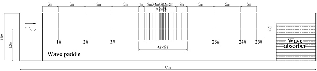
Figure 1. Sketch of the experimental setup.

Generation of Double Wave Groups Focusing

The free surface elevation of double wave groups focusing can be achieved by the superposition of the corresponding single wave group. The single wave group can be expressed as Rapp and Melville (1990):

$\begin{array}{ll}\eta (x,t)={\displaystyle \sum _{i=1}^{N_f}}{a}_{i}cos\left[k_i(x-x_b)-2\pi f_i(t-t_b)\right]& (1)\end{array}$

where the subscript i stands for the i-th wave component. N_f is the total number of wave components in a single wave group. x_b and t_b are the assumed wave focusing location and time, respectively. a_i, k_i, and f_i are the wave amplitude, wave number and wave frequency of each component. The value of k_i can be obtained through the dispersion equation:

$\begin{array}{ll}{(2\pi f_i)}^2=g{k}_{i}th{k}_{i}h& (2)\end{array}$

where h is the water depth.

In this paper, wave groups are considered to be uni-directional, the wave amplitude of each component a_i is determined by the wave spectrum S(f) using the following equation:

$\begin{array}{ll}{a}_i=A_b\frac{S(f_i)\Delta f}{{\displaystyle \sum _{n=1}^{N_f}}S(f_n)\Delta f}& (3)\end{array}$

where A_b is the assumed focusing wave amplitude. S(f) is a JONSWAP spectrum (Goda, 1999), which is expressed as:

$\begin{array}{ll}S(f)=\alpha H_{1/3}^2{T}_P^{-4}{f}^{-5}exp\left[-\frac{5}{4}{(T_{p}f)}^{-4}\right]{\gamma }^{exp\left[-{(f/f_p-1)}^2/(2{\sigma }^2)\right]}& (4)\end{array}$

where α = 0.06238/[0.230+0.0336γ−0.185(1.9+γ)] (1.094–0.01915lnγ), σ = 0.07 (f < f_p), and σ = 0.09 (f ≥ f_p). H_1/3 is the significant wave height, here normalized as H_1/3 = 1 to achieve the wave amplitude of each component a_i in Equation (3). T_p is the peak wave period corresponding to the peak frequency f_p. The shape parameter γ = 3.3 is used in this paper. Equation (3) indicates that the distribution of the amplitude over frequency or amplitude spectrum takes the same shape with that of the used wave spectrum.

Two single wave groups defined by Equation (1) are focused at the same location and time to generate focused waves. In the experiment, displacement of wavemaker, X(t), of these two single wave groups are superimposed together directly. Double wave groups of different frequencies are generated and propagated up to the region of wave focusing. In the region of wave focusing, the wave energy of two wave trains is concentrated, and consequently, focusing waves can be produced in both experimental and numerical simulation.

Wave Conditions

The experiment in this paper contains two parts: individual single wave group focusing and double wave groups focusing. All experimental parameters are given in Table 1. Table 1(A) lists wave parameters of individual single wave group focusing, with target wave focusing time, location, and discretization of the wave spectrum. Four cases with different wave amplitudes and peak frequencies f_p are considered. Appropriate focusing amplitudes A_b are chosen so that there is no wave breaking during the process of the double wave groups focusing. Positive value of A_b means crest focusing. In the experiment, corresponding trough focusing is generated by multiplying the wavemaker signal of crest focusing with −1. k_p and L_p are the wave number and the wavelength corresponding to the peak frequency, respectively. Due to the non-linearity in the propagation of the wave trains, the actual focusing location will have a small shift from the input focusing location. The experiments of individual single wave group focusing are adjusted by the correction of the input focusing location and time, to ensure the wave groups of these four different cases to be focused at the same position (x_b = 22 m) and time (t_b = 60 s). Wave spectra are discretized in the same frequency range (0.4–2.0 Hz) with the same number of wave components N_f = 200. Wave frequencies are uniformly discretized in the frequency region.

TABLE 1

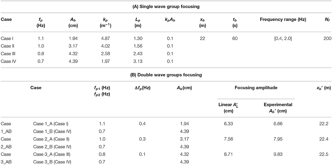
Table 1. Experimental parameters.

And then input the new wavemaker signals, composed by the superimposition of the first three cases (CaseI, Case II, and Case III) with that of the last case (Case IV) respectively, into the wavemaker system to produce the double wave groups focusing in the experimental flume. The experimental cases for double wave groups focusing are listed in Table 1(B). “Case_A” and “Case_B” stand for the cases of single wave group propagation, respectively. “Case_AB” stands for the case of double wave groups focusing. The term f_p1 and f_p2 are peak frequencies of the high-frequency group and the low-frequency group, respectively. Δf_p (=f_p1-f_p2) is the difference between the two peak frequencies. Figure 2 presents the displacement time series of the wavemaker for Case 1_AB. The upper figure shows wavemaker displacement for two individual single wave group focusing, and the lower figure shows the superposed wavemaker displacement to generate focused double wave groups.

FIGURE 2

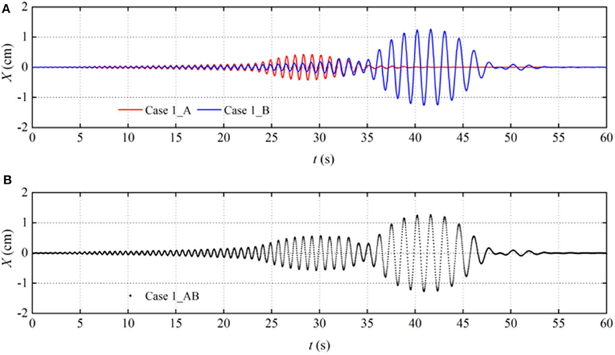
Figure 2. Wavemaker (x = 0 m) displacement of the (A) independent single wave group focusing and (B) double wave groups focusing for Case 1.

The actual amplitude spectra measured at 5.0 m away from the wavemaker for these three cases [listed in Table 1(B)] are illustrated in Figure 3. As the difference between the two peak frequencies Δf_p is larger, the two peak amplitude spectra become evident. Table 1(B) also lists the measured focusing amplitude and location of these three double wave groups. The actual focusing amplitudes from the experiment A_b′ are larger than those obtained from the linear sum of the corresponding single wave group A_L′, and the actual focusing locations x_b′ are shifted in the downwind direction from the focusing location of the corresponding single wave group. With the fixed steepness (i.e., the same non-linear strength), the changes in the focusing amplitude and location are related to the differences between the two peak frequencies Δf_p. They increase as Δf_p values decrease. This phenomenon is mainly caused by the interactions between two single wave groups, which will be explained in the following section.

FIGURE 3

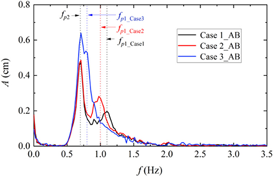
Figure 3. Actual amplitude spectra at the location x = 5.0 m for different peak frequently differences.

Results and Analysis

Evolution of the Wavelet Spectra

To investigate the evolution process during wave propagation, wavelet transform (WT) analysis is used. WT analysis is suitable for wave data of non-Gaussian, non-stationary, transient phenomena like freak waves. As the mother wavelet function, Morlet wavelet is used to analyze wave data given as the below (Torrence and Compo, 1998; Li et al., 2015):

$\begin{array}{ll}\psi (t)={\pi }^{\text{-}\frac{1}{4}}exp\left(-\frac{t^2}{2}\right)exp(i{\omega }_{0}t)& (5)\end{array}$

where ω₀ is the frequency of the mother wavelet, and its value depends on the input spectrum in the analysis.

Wavelet spectra at different locations for Case 1_AB are presented in Figure 4. From Figure 4A, it can be observed that, at the location near the wavemaker (x = 3.0 m), one wave group with high frequency components is followed by the other one with low frequency components, and these two wave groups are almost completely separated. As the wave propagates, the low frequency group catches up with the high frequency group. The energy of two successive groups are approaching gradually, and the amplitude of waves increases in Figure 4B. At the focusing location x = 22.2 m, the wavelet power becomes sharp, and the largest wave is measured which has the typical “three sisters” form in Figure 4C (Haver, 2004). High frequency components can be found obviously in the wavelet spectra. After wave focusing, the two wave groups begin to separate. Eventually, the low frequency group is followed by the high frequency group. Evolutions of the wavelet spectra are consistent with those of the freak wave formation in random wave trains shown in Li et al. (2015). This implies that the focusing of the double wave groups can reproduce the generation process of the freak waves in random wave trains well.

FIGURE 4

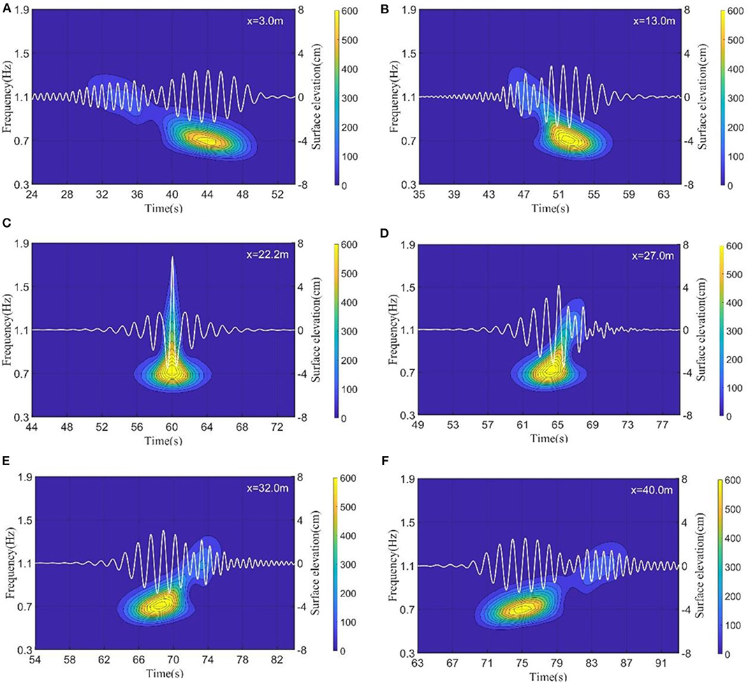
Figure 4. Wavelet spectra at different locations for Case 1_AB. (A) x = 3.0 m, (B) x = 13. 0 m, (C) x = 22.2 m, (D) x = 27.0 m (E) x = 32.0 m and (F) x = 40.0 m.

Comparison of the Free Surface Elevation

Figure 5 compares the time history of the free surface elevation between the linear superposition of the corresponding single wave group focusing listed in Table 1(A) (black solid lines) and the actual experimental data of the double wave groups focusing (red solid lines) for three cases listed in Table 1(B). At the location near the wavemaker (x = 3.0 m), the red and black lines are almost identical, indicating that the interactions between the two wave groups are very small. After wave focusing, there are obvious phase lags between these two focusing processes, especially for the high frequency group. The phase lag remains after two wave groups are separated. This may be caused by the high order non-linearity due to the interaction between two wave groups (i.e., the high order waves that no longer obey the linear dispersion relationship) during the wave focusing process. It will be analyzed quantitatively in a later section. Furthermore, the non-linear interactions mainly affect the high frequency components, therefore obvious phase lag is observed for the high frequency part of the double wave groups.

FIGURE 5

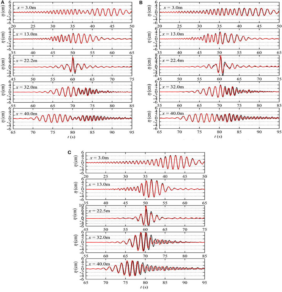
Figure 5. The comparisons of the surface elevations between the linear superposition of the corresponding single wave group focusing and the double wave groups focusing (black solid lines represent the linear superposition of single wave group focusing, and red solid lines represent the double wave groups focusing). (A) Case 1_AB, (B) Case 2_AB, (C) Case 3_AB.

Analysis of the Amplitude Spectra

The amplitude spectra of the double focused groups and those of the corresponding single group at different locations for Case 1_AB are illustrated in Figure 6. In order to facilitate a more detailed observation, amplitude spectra are given in both a linear scale (on the left side of the figure) and a semi-log scale (on the right side of the figure). The vertical dotted lines represent the peak frequencies of the corresponding single wave group. The amplitude spectra of two single wave groups experience almost no changes during the wave focusing process. In contrast, the amplitude spectra change during the process of the double wave groups focusing (see Figure 6C). As the double wave groups approach the focusing location and the two wave groups begin to interact, the peak amplitude on its left side of the high frequency group (0.8–1.1 Hz) gradually decreases, while the amplitude of higher frequency (1.2–3.0 Hz) components increase. Consequently, the energy of the high frequency (0.8–1.1 Hz) components transfer to the higher frequency (1.2–3.0 Hz) components. At the focusing location, the interaction between the two wave groups becomes strong, and the change of the amplitude spectrum is obvious. After wave focusing, the amplitude spectra are similar to the one before the wave focusing. It can be noted that the amplitude spectra of the low frequency (0.5–0.8 Hz) components experience almost no changes during the whole process. Similar phenomena are observed for Case 2_AB and Case 3_AB, and the amplitude spectra during the wave focusing are given in Figure 7. Similar to Case 1_AB, significant changes also occur in the higher frequency region, especially at the focusing location, while there is a small change in the low frequency part during the focusing process.

FIGURE 6

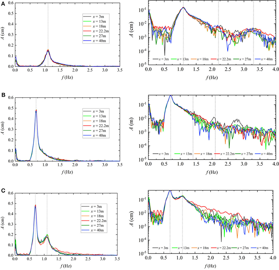
Figure 6. The amplitude spectra at different locations along the wave flume for (A) Case 1_A, (B) Case 1_B, and (C) Case 1_AB.

FIGURE 7

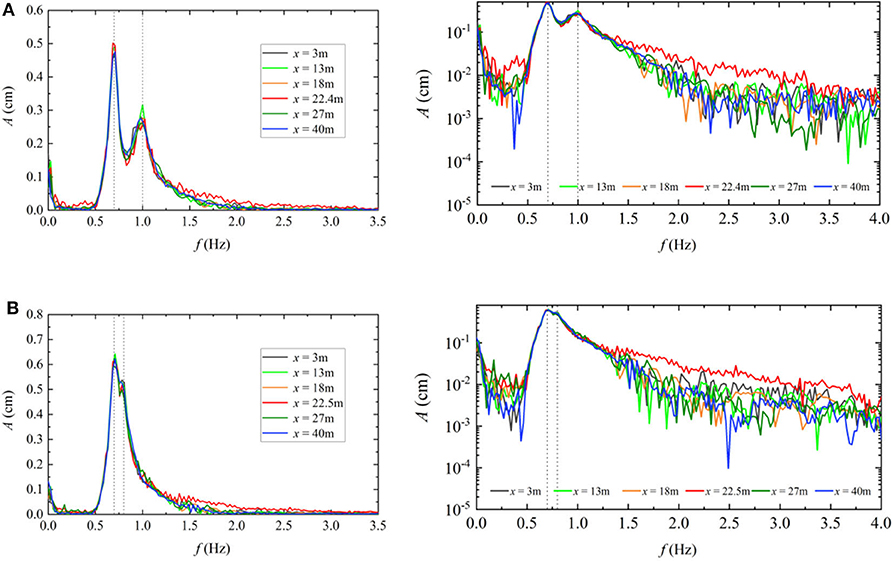
Figure 7. The amplitude spectra at different locations along wave flume for (A) Case 2_AB and (B) Case 3_AB.

Separation of the Harmonic Components

The above observation implies that there are strong non-linear interactions between two wave groups during the wave focusing process. To further analyze the non-linear interactions, a method for the symmetry-based separation of harmonics is used to separate the different harmonic components of the free surface for the focused waves (Johannessen and Swan, 2003; Fitzgerald et al., 2014; Zhao et al., 2017). According to their method, the free surface elevation of the crest focused group η_(c) and trough focused group η_(t) can be expressed as:

$\begin{array}{l}{\eta }_{(c)}={\displaystyle \sum _i}{G}_1(a_i,k_i,h)+{\displaystyle \sum _i}{\displaystyle \sum _j}{G}_2(a_i{a}_j,k_i,k_j,h)\\ +{\displaystyle \sum _i}{\displaystyle \sum _j}{\displaystyle \sum _l}{G}_3(a_i{a}_j{a}_l,k_i,k_j,k_l,h)+...& (6)\end{array}$

$\begin{array}{l}{\eta }_{(t)}=-{\displaystyle \sum _i}{G}_1(a_i,k_i,h)+{\displaystyle \sum _i}{\displaystyle \sum _j}{G}_2(a_i{a}_j,k_i,k_j,h)\\ -{\displaystyle \sum _i}{\displaystyle \sum _j}{\displaystyle \sum _l}{G}_3(a_i{a}_j{a}_l,k_i,k_j,k_l,h)-...& (7)\end{array}$

where G represents functions of the amplitudes a_i, wave number vectors k_i, and water depth h, respectively. Therefore, the function G can represent the various interactions of different wave components during the wave focusing event. It is worth noting that the non-linearities up to third order are extracted in the present study.

Hence, odd terms, including the first-order components and the third-order components, can be extracted by:

$\begin{array}{l}{\eta }_{(odd)}=\frac{{\eta }_{(c)}-{\eta }_{(t)}}{2}={\displaystyle \sum _i}{G}_1(a_i,k_i,h)\\ +{\displaystyle \sum _i}{\displaystyle \sum _j}{\displaystyle \sum _l}{G}_3(a_i{a}_j{a}_l,k_i,k_j,k_l,h)+oddterms& (8)\end{array}$

where G₃ includes the third-order bound components and the third-order resonant components. Similarly, even terms, including the second-order components, are obtained from:

$\begin{array}{ll}{\eta }_{(even)}=\frac{{\eta }_{(c)}+{\eta }_{(t)}}{2}={\displaystyle \sum _i}{\displaystyle \sum _j}{G}_2(a_i{a}_j,k_i,k_j,h)\text{+}eventerms& (9)\end{array}$

Based on Equations (8) and (9), the wave surface representing the odd-order and even-order waves can be analyzed according to the measured crest and trough focusing waves.

According to the research by Zhao et al. (2017), there are cross-terms in each harmonic component, which have the same frequency, but a different (higher-order) dependence on the wave amplitude. For example, a third-order interaction of three linear components results in a term that scales as the cube of the linear wave amplitude, but its frequency component is in the linear range. In general, all such cross-terms are likely to be negligible for weakly non-linear waves, except for the second-order difference term (zeroth harmonic) bound to the fourth harmonic (Zhao et al., 2020). Hence, the difference between the odd-order components and the linear superposition result is mainly in the third-order non-linearity due to interactions between two wave groups.

The amplitude spectra of the odd-order terms and even-order terms of the double wave groups focusing for Case 1_AB are analyzed in Figure 8A. Compared to Figure 6C, there are similar changes in the amplitude spectra of the odd-order term, especially in the region of 0.8–2.0 Hz. This means that the main changes in the amplitude spectra of the wave components during wave focusing are caused by the third-order non-linearity. The slight changes in 2.0–3.0 Hz that occur in Figure 6C are observed in the amplitude spectra of the even-order terms, implying that these changes are caused by the second-order non-linearity due to interactions between wave groups. While, compared with the third-order non-linearity, the second-order non-linearity is not obvious. There are similar phenomena for Case 2_AB and Case 3_AB in Figures 8B,C.

FIGURE 8

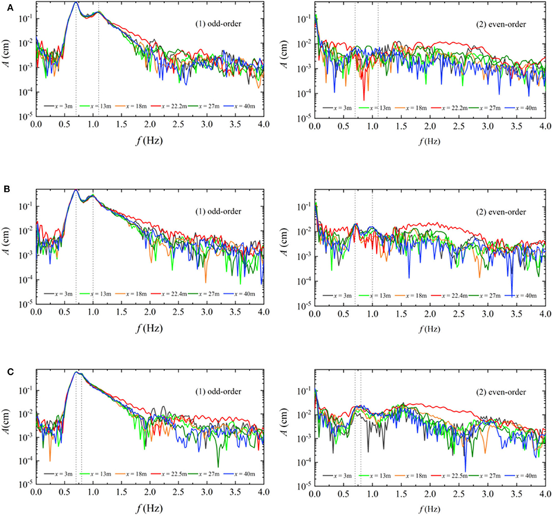
Figure 8. The amplitude spectra of the odd- and even-order components. (A) Case 1_AB, (B) Case 2_AB, (C) Case 3_AB.

The above observations show that third-order non-linearity plays a significant role in double wave groups focusing. In Figure 9, the analyzed wave surface elevations of the odd-order components of the focused double wave groups for the three cases are compared with those of the focused double wave groups. The odd-order components clearly always have the same phase with that of the focused double wave groups, irrespective of occurring before or behind the focusing location. This phenomenon further confirms the fact that the third-order non-linearity causes the phase lags for the wave surface elevation.

FIGURE 9

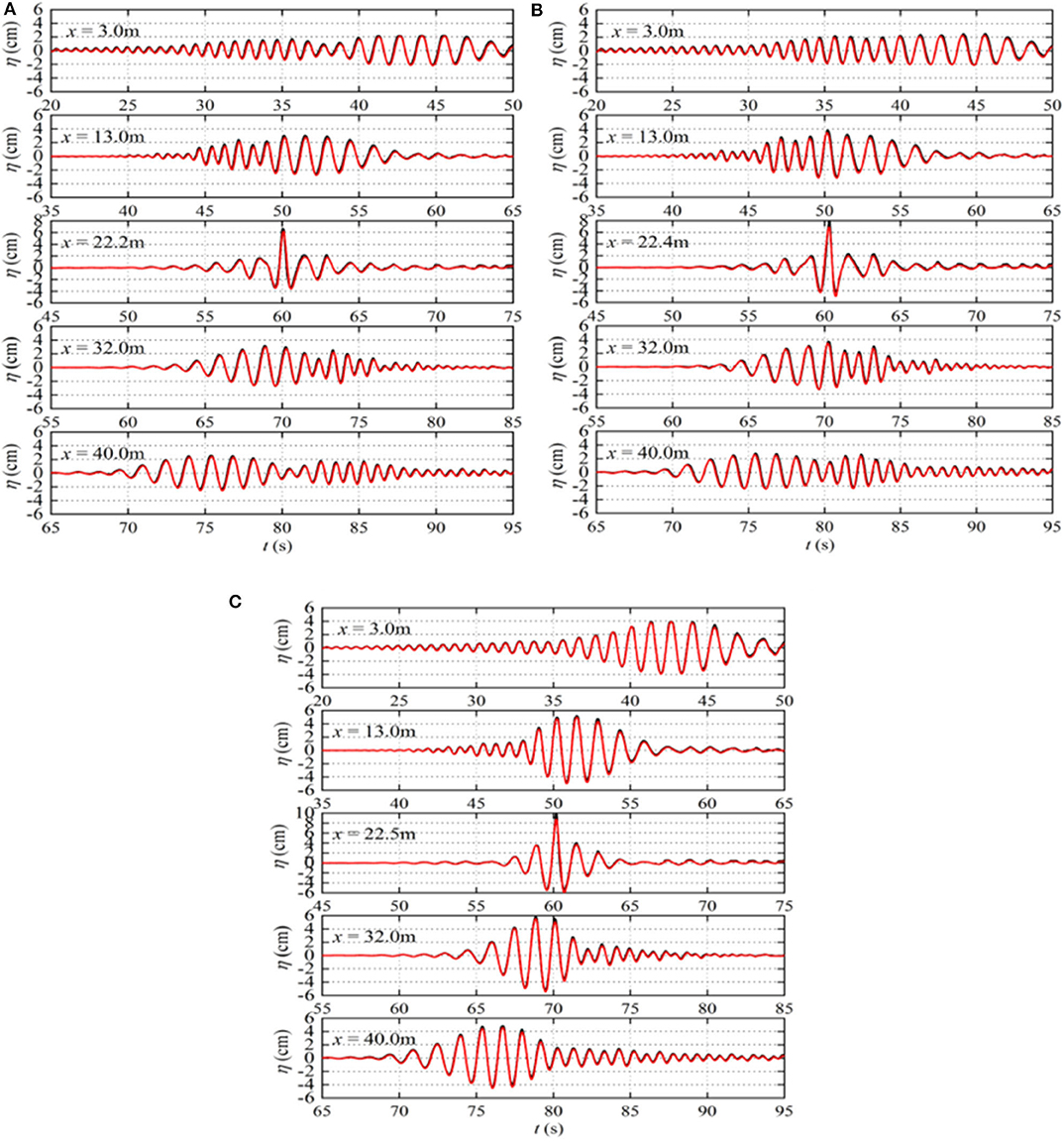
Figure 9. The comparions of the free surface elevations between the focused double wave groups and the odd-order components of the focused double wave groups (black solid lines represent the focused double wave groups, and red solid lines represent the odd-order components of the focused double wave groups). (A) Case 1_AB, (B) Case 2_AB, (C) Case 3_AB.

Analysis of the Phase Shift

The cross-spectral density function S_xy(f) can be used to analyze the phase shift between the two wave groups. S_xy(f) is the Fourier transform of the cross-correlation function of two time series x(t) and y(t). S_xy(f) represents the phase difference between x(t) and y(t), obtained by conjugate multiplication of the spectrum of the x(t) signal and that of the y(t) signal. If x(t) and y(t) are real functions, S_xy(f) is always a complex function:

$\begin{array}{ll}{s}_{xy}(f)=C_{xy}(f)-i{Q}_{xy}(f)& (10)\end{array}$

in which C_xy(f) is the co-spectral density function, and Q_xy(f) is the quad-spectral density function.

The time delay in the time domain contributes to the phase shift in the frequency domain. Thus, the phase spectrum θ_xy(f) indicates the phase shift of y(t) relative to x(t):

$\begin{array}{ll}{\theta }_{xy}(f)=\text{arctan}\left\{Q_{xy}(f)/C_{xy}(f)\right\}& (11)\end{array}$

According to Equation (11), the phase shift of the double wave groups focusing [AB, i.e., y(t)] relative to the linear superposition of the corresponding single wave group [A+B, i.e., x(t)] can be calculated. Figure 10 shows the phase shift of different frequency components at different locations for these three cases. At the locations near the wavemaker (x = 3.0 m), there are no phase shifts in the range of the fundamental frequency. The phase shifts increase slightly for the high frequency components as the wave propagation and significant phase shift is observed during the wave focusing process. It conforms to the phenomenon observed from Figure 5, that the phase shift obviously appears in the high frequency part of the initial spectral band.

FIGURE 10

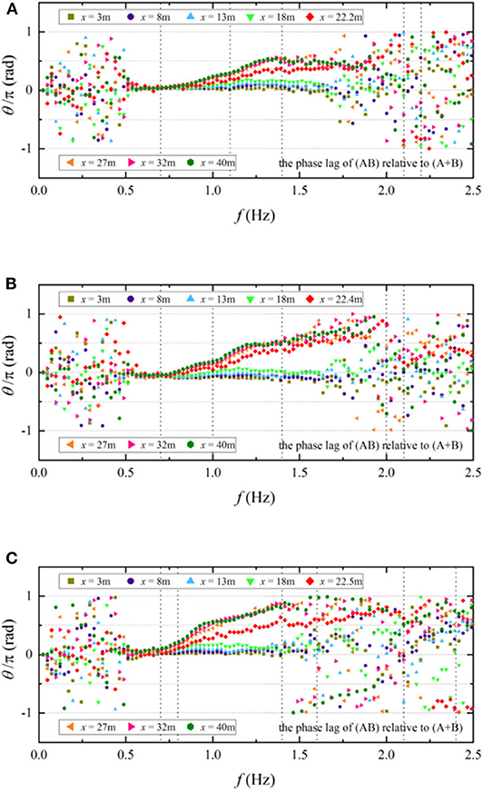
Figure 10. The phase lag of the double wave groups focusing [AB, i.e., y(t)] relative to the linear superposition of the corresponding single wave group [A+B, i.e., x(t)]. (A) Case 1_AB, (B) Case 2_AB, (C) Case 3_AB.

Figure 11 compares the phase shift of selected frequency components (the first one, f = 0.7 Hz, is the peak frequency of the low-frequency group, the second one is the peak frequency of the high-frequency group, and the third one, f = 1.4 Hz, is twice the peak frequency of the low-frequency group) at different locations along the wave flume. For the low frequency component f = 0.7 Hz, the phase shifts remain almost 0 along the wave flume. This proves that there is no third-order non-linearity for this wave component, and this wave component always obeys the linear dispersion relationship during the interactions of the two wave groups. Additionally, for higher frequency components, the phase shifts are also 0 at locations in front of the focusing location. As the wave groups approach the focusing location, phase shifts increase rapidly, which reflects that there is strong third-order non-linearity for these high wave components when two wave groups are focused together. After passing by the focusing location, the third-order non-linear interaction between waves becomes weak as two wave groups are separated. The phase shifts stay almost constant, and the wave components propagate with the new phase.

FIGURE 11

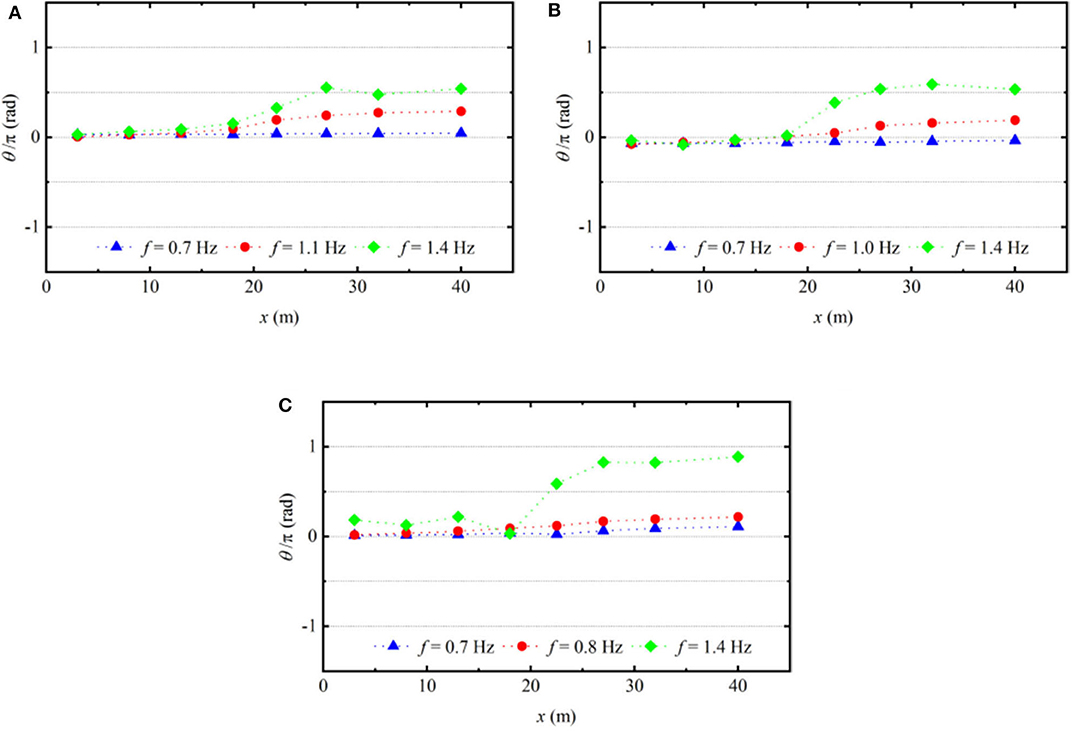
Figure 11. The phase lag of the focused double wave groups relative to the linear superposition of the corresponding single wave group for selected frequencies along the wave flume. (A) Case 1_AB, (B) Case 2_AB, (C) Case 3_AB.

Comparing the results of different cases, it also can be observed that with the fixed steepness of each independent focusing group, the case with a small peak frequency difference has a larger phase shift than cases of large peak frequency differences. This states that there is stronger third-order non-linearity due to interactions between two wave groups for the double wave groups with a small peak frequency difference, leading to a large shift from the input focusing location.

Numerical Simulation

From the above analysis for the experimental data, phase shifts occur in the non-linear process of the double wave groups focusing. In order to further investigate the changes of the dispersion relationship, focused waves generated by double wave groups are simulated in a numerical wave tank based on the HOS method.

Numerical Model

Ducrozet et al. (2012) and Li and Liu (2015) have enhanced the initial HOS method proposed by Dommermuth and Yue (1987) and West et al. (1987) to represent a water wave tank, including a wave maker and an absorbing beach. In their models, the velocity potential is split into the sum of a previously described spectral potential component Φ_f and a prescribed non-periodic component Φ_w. Then the free surface boundary conditions can be expressed as:

$\begin{array}{ll}\frac{\partial \eta }{\partial t}=(1+{\left|{\nabla }_x\eta \right|}^2)\frac{\partial {\Phi }_f^s}{\partial z}+\frac{\partial {\Phi }_w}{\partial z}-{\nabla }_x({\Phi }_f^s+{\Phi }_w)·{\nabla }_x\eta z=\eta & (12)\end{array}$

$\begin{array}{ll}\begin{array}{c}\frac{\partial {\Phi }_f^s}{\partial t}=-\frac{1}{2}{\left|{\nabla }_x{\Phi }_f^s\right|}^2+\frac{1}{2}(1+{\left|{\nabla }_x\eta \right|}^2){(\frac{\partial {\Phi }_f^s}{\partial z})}^2-{\nabla }_x{\Phi }_f^s·{\nabla }_x{\Phi }_w\\ -\frac{\partial {\Phi }_w}{\partial t}-\frac{1}{2}{\left|{\nabla }_x{\Phi }_w\right|}^2-\frac{1}{2}{(\frac{\partial {\Phi }_w}{\partial z})}^2-g\eta z=\eta \end{array}& (13)\end{array}$

The bottom boundary condition satisfies:

$\begin{array}{ll}\nabla \Phi ·\vec{n}=0& (14)\end{array}$

where $\overrightarrow{n}$ is a vector normal to the corresponding boundary.

The wavemaker boundary condition can be written as:

$\begin{array}{ll}\frac{\partial \Phi }{\partial x}=\frac{\partial X(t)}{\partial t}onx=0& (15)\end{array}$

According to the linear wave-maker theory (Dean and Dalrymple, 1984), the velocity of the wavemaker can be calculated by:

$\begin{array}{ll}\frac{\partial X(t)}{\partial t}=\frac{\omega }{T(k)}{\eta }^{\prime }& (16)\end{array}$

where η′ is the expected wave surface elevation, and T(k) is the transfer function for a piston-type wavemaker and can be calculated by:

$\begin{array}{ll}T(k)\text{=}\frac{2\left[cosh(2kh)-1\right]}{2kh+sinh(2kh)}& (17)\end{array}$

The unknown component Φ_f can be solved using the traditional HOS method proposed by Dommermuth and Yue (1987). And the non-periodic component Φ_w can be calculated regarding Bonnefoy's (Bonnefoy et al., 2010) method.

The details of this numerical model can be found in Li and Liu (2015).

Numerical Validation

The experimental results of Case 1_AB are used to validate the accuracy of the numerical model. In the numerical simulation, the wave tank is 80 m long with a water depth of 1.2 m. Spatial discretization in the horizontal direction Δx is adopted as 0.05 m, and the time step Δt is 0.01 s. The non-linear order of the HOS method is taken as 8. The total simulation duration is 140 s. Comparison of the free surface elevations at different locations between the numerical results and experimental data is presented in Figure 12. It can be observed that the numerical results agree quite well with the experimental data along the wave tank to reproduce the process of the wave focusing accurately. This validation underlines the applicability of the established HOS numerical model toward simulating the evolution of two focused wave groups.

FIGURE 12

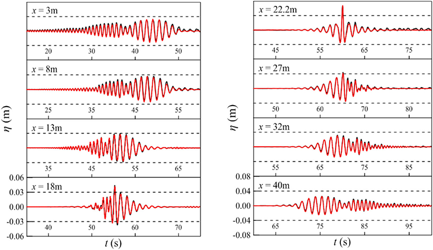
Figure 12. Comparison of the free surface elevations between the numerical results and physical experimental data along the wave tank for Case 1_AB (black solid lines represent the experimental data, and red solid lines represent the numerical results).

Analysis of the Dispersion Relationship

As aforementioned, the third-order non-linearity causes the phase lags for the wave surface elevation, which means changing the dispersion relationship in the process of the double wave groups focusing. In order to illustrate the changes of the dispersion relationship, the analysis of the wavenumber-frequency (k-f) spectrum is performed, referring to Swan (2007).

The wavenumber-frequency (k-f) spectrum, obtained by 2D Fourier transforms in time and space, includes information of each wave component both in time and space. Hence, both the evolution of the amplitude spectra and changes to the dispersive properties of the wave groups can be identified through a k-f spectrum, providing a comprehensive understanding of the non-linear coupling effect between different frequencies.

The k-f spectra of the simulated double wave groups for Case 1_AB are shown in Figure 13A, in which the location and time at which and when the transform is applied are indicated in the lower right corner. Therein, the blue dashed lines indicate the linear dispersion relationship. In these subplots, a number of identifiable “ridges” representing different frequency components can be obviously observed. For instance, at x = 22.2m, “ridges” represent the third-order sum components, the second-order sum components, the free wave components, and the second-order difference components in order from top to bottom.

FIGURE 13

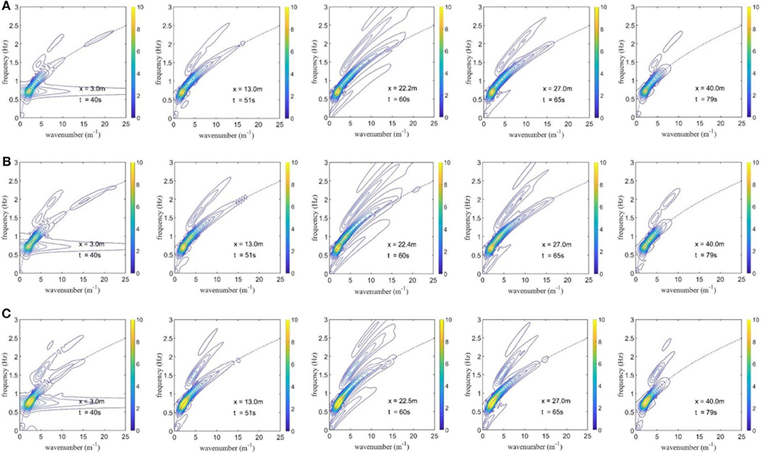
Figure 13. Wavenumber-frequency spectra at typical locations along the numerical wave tank (blue dashed lines indicate the linear dispersion relationship). (A) Case 1_AB, (B) Case 2_AB, (C) Case 3_AB.

The subplots in Figure 13A illustrate that the non-linear interactions are weak and the higher order wave components are not significant before wave focusing. The free wave components also satisfy the linear dispersion relationship. At the focusing location x = 22.2 m, due to the strong interaction, the higher order wave components become significant, and the free wave components deviation from the linear dispersion relationship increases in the high frequency region. This demonstrates that the non-linear interactions change the dispersion relationship of the wave components, leading smaller wavenumbers than the linear case during the wave focusing process. After the focusing location, the energy of the higher order components transfer to the high order components and the wavenumber-frequency follows the linear relationship as the two wave groups are separated. Similar phenomena can be discovered in Figures 13B,C for Case 2_AB and Case 3_AB.

In addition, wavenumber-frequency (k-f) spectra at the focusing location of the odd-order components for these three cases with different peak frequency widths are given in Figure 14. The changes in dispersion for free wave components are consistent with those in Figure 13. This intuitively explains that the third-order non-linearity, here including the bound as well as resonant effect, due to the interactions between two wave groups changes the dispersion relationship during the wave focusing process. This is identical to that obtained by Swan (2007), who noted that the third-order resonant effects dominate changes to both the amplitude of the wave components and the dispersive properties of the wave group.

FIGURE 14

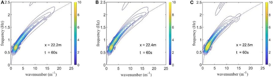
Figure 14. Wavenumber-frequency spectra at the focusing location of odd-order components for different cases (blue dashed lines indicate the linear dispersion relationship). (A) Case 1_AB, (B) Case 2_AB, (C) Case 3_AB.

Conclusions and Discussions

Based on the previous experimental observation (Li et al., 2015), a modified wave focusing experiment is proposed to simulate the generation of freak waves in this study. As a supplement to the previous focusing methods (Rapp and Melville, 1990; Baldock et al., 1996), the experiment contains two parts: individual single wave group focusing and double wave groups focusing. Individual single wave group with different peak frequencies (f_p = 1.1, 1.0, 0.8, and 0.7 Hz) is adjusted to be focused at the same location and time by correction of the target focusing values. And then input the new wavemaker signals, composed by the superimposition of the first three cases (f_p = 1.1, 1.0, and 0.8 Hz) with that of the last case (f_p = 0.7 Hz) respectively, to the wavemaker system to produce the double wave groups focusing in the experimental flume.

Wavelet analysis of the double wave groups focusing is consistent with that of the freak wave formation in random wave trains in Li et al. (2015), indicating that double wave groups focusing can also reproduce the freak wave generation process well. By comparing the free surface elevations and the amplitude spectra of the double wave groups focusing with those of the linear superposition of the corresponding single wave group, phase lags and spectral changes in the high frequency part of the double wave groups can be obviously observed during the focusing process. Thanks to the separation of wave harmonics for focused waves, the non-linearity due to interactions between two wave groups is further explored. Phase lags are attributed to the odd-order (mainly the third-order), rather than the even-order non-linearity, leading to a small wavenumber during the focusing process. Additionally, the analysis of the phase shifts illustrates that the changes resulted from third-order non-linearity mainly occur in the high frequency components, so the low frequency part of the double wave groups almost appears no changes in the process of double wave groups focusing. With regards to the high frequency part, although the amplitudes of the wave components recover to the initial state after wave focusing, the change of phases remains. These phenomena are obvious for the cases with small peak frequency differences, which confirms the fact that the freak waves occur more easily in a sea with a narrow-band spectrum. The above observations are also verified by the analysis of the results from the numerical simulation based on the HOS method. Wavenumber-frequency spectra comprehensively present the identifiable “ridges” representing different frequency components, involving their emergence, growth and disappearance in the process of double wave group focusing. Meanwhile, the wavenumber-frequency spectra of the odd-order components represent a quantitative description of the changes in the dispersive properties and the evolution of the amplitude spectra during the focusing process. It can be more intuitively observed the third-order non-linear coupling effect between different frequencies.

All these observations provide a better understanding of the non-linear interaction between wave groups in random wave trains and also of the generation mechanism of freak waves. Furthermore, it also can provide theoretical support for evaluating the endurance limit of the wave energy devices to reduce the damage and unnecessary losses as much as possible, so as to promote the efficient and sustainable development of marine energy resources.

Data Availability Statement

The datasets generated for this study are available on request to the corresponding author.

Author Contributions

Y-PF conducted the physical experiment. LW performed the data processing and numerical analysis. LW wrote the manuscript draft. J-XL and S-XL provided research guidance and advice. All authors contributed to the manuscript revisions, read, and approved the submitted version.

Funding

This research was supported by National Key R&D Program of China (2016YFC1401405, 2016YFE0200100), the National Natural Science Foundation of China (51739010, 51879037), and the Fundamental Research Funds for the Central Universities of China.

Conflict of Interest

The authors declare that the research was conducted in the absence of any commercial or financial relationships that could be construed as a potential conflict of interest.

References

Adcock, T. A. A., and Taylor, P. H. (2014). The physics of anomalous (‘rogue’) ocean waves. Reports Progress Phys. 77:105901. doi: 10.1088/0034-4885/77/10/105901

PubMed Abstract | CrossRef Full Text | Google Scholar

Baldock, T. E., Swan, C., and Taylor, P. H. (1996). A laboratory study of nonlinear surface waves on water. Philos. Trans. Roy. Soc. A 354, 649–676. doi: 10.1098/rsta.1996.0022

CrossRef Full Text | Google Scholar

Benjamin, T. B., and Feir, J. E. (1967). The disintegration of wave trains on deep water. Part 1: Theory. J. Fluid. Mech. 27, 417–430. doi: 10.1017/S002211206700045X

CrossRef Full Text | Google Scholar

Bitner-Gregersen, E. M., and Toffoli, A. (2014). Occurrence of rogue sea states and consequences for marine structures. Ocean Dynamics 64, 1457–1468. doi: 10.1007/s10236-014-0753-2

CrossRef Full Text | Google Scholar

Bonnefoy, F., Ducrozet, G., Le Touzé, D., and Ferrant, P. (2010). Time domain simulation of nonlinear water waves using spectral methods. Adv. Num. Sim. Nonlin. Water Waves 11, 129–164. doi: 10.1142/9789812836502_0004

CrossRef Full Text | Google Scholar

Cruz, J. (2008). Ocean wave energy: current status and future prespectives. Bull. Acad. Nat. Méd. 196, 1709–1720. doi: 10.1007/978-3-540-74895-3

CrossRef Full Text | Google Scholar

Dean, R. G., and Dalrymple, R. A. (1984). Water Wave Mechanics for Engineers and Scientists. Singapore: Prentice-hall Inc. doi: 10.1142/1232

CrossRef Full Text | Google Scholar

Dommermuth, D. G., and Yue, D. K. P. (1987). A High-Order Spectral method for the study of nonlinear gravity waves. J. Fluid Mech. 184, 267–288. doi: 10.1017/S002211208700288X

CrossRef Full Text | Google Scholar

Ducrozet, G., Bonnefoy, F., Le Touzé, D., and Ferrant, P. (2012). A modified High-Order Spectral method for wave-maker modeling in a wave tank. Eur. J. Mechan. B/Fluids 34, 19–34. doi: 10.1016/j.euromechflu.2012.01.017

CrossRef Full Text | Google Scholar

Dyachenko, A. I., and Zakharov, V. E. (2005). Modulation instability of Stokes wave freak wave. J. Exp. Theor. Phys. Lett. 81, 255–259. doi: 10.1134/1.1931010

CrossRef Full Text | Google Scholar

Dysthe, K., Krogstad, H. E., and Müller, P. (2008). Oceanic rogue waves. Annu. Rev. Fluid Mech. 40, 287–310. doi: 10.1146/annurev.fluid.40.111406.102203

CrossRef Full Text | Google Scholar

Fitzgerald, C. J., Taylor, P. H., Eatock Taylor, R., Grice, J., and Zang, J. (2014). Phase manipulation and the harmonic components of ringing forces on a surface-piercing column. Proc. Roy. Soc. A Mathem. Phys. Eng. Sci. 470, 20130847–20130847. doi: 10.1098/rspa.2013.0847

CrossRef Full Text | Google Scholar

Goda, Y. (1999). A comparative review on the functional forms of directional wave spectrum. Coas. Eng. J. 41, 1–20. doi: 10.1142/S0578563499000024

CrossRef Full Text | Google Scholar

Haver, S. (2004). “A possible freak wave event measured at the Draupner Jacket January 1 1995,” in Rogue Waves 2004: Proceedings of a Workshop Organized by Ifremer and Held in Brest (France), 1–8.

Google Scholar

Johannessen, T. B., and Swan, C. (2003). On the nonlinear dynamics of wave groups produced by the focusing of surface-water waves. Proc. Roy. Soc. A Mathem. Phys. Eng. Sci. 459, 1021–1052. doi: 10.1098/rspa.2002.1028

CrossRef Full Text | Google Scholar

Kharif, C., and Pelinovsky, E. (2003). Physical mechanisms of the rogue wave phenomenon. Eur. J. Mech. B/Fluids 22, 603–634. doi: 10.1016/j.euromechflu.2003.09.002

CrossRef Full Text | Google Scholar

Li, J. X., and Liu, S. X. (2015). Focused wave properties based on a High Order Spectral method with a non-periodic boundary. China Ocean Eng. 29, 1–16. doi: 10.1007/s13344-015-0001-7

CrossRef Full Text | Google Scholar

Li, J. X., Yang, J. Q., Liu, S. X., and Ji, X. R. (2015). Wave groupiness analysis of the process of 2D freak wave generation in random wave trains. Ocean Eng. 104, 480–488. doi: 10.1016/j.oceaneng.2015.05.034

CrossRef Full Text | Google Scholar

Onorato, M., Cavaleri, L., Fouques, S., Gramstad, O., Janssen, P. A. E. M., Monbaliu, J., et al. (2009). Statistical properties of mechanically generated surface gravity waves: a laboratory experiment in three-dimensional wave basin. J. Fluid Mech. 627, 235–257. doi: 10.1017/S002211200900603X

CrossRef Full Text | Google Scholar

Onorato, M., Osborne, A., Serio, M., Cavaleri, L., Brandini, C., and Stansberg, C. (2006). Extreme waves, modulational instability and second order theory: wave flume experiments on irregular waves. Eur. J. Mechan. B/Fluids 25, 583–601. doi: 10.1016/j.euromechflu.2006.01.002

CrossRef Full Text | Google Scholar

Osborne, A. R. (2001). The random and deterministic dynamics of ‘rogue waves’ in unidirectional deep-water wave trains. Mar. Struct. 14, 275–293. doi: 10.1016/S0951-8339(00)00064-2

CrossRef Full Text | Google Scholar

Rapp, R. J., and Melville, W. (1990). Laboratory measurements of deep-water breaking waves. Proc. Roy. Soc. A Mathem. Phys. Eng. Sci. 331, 735–800. doi: 10.1098/rsta.1990.0098

CrossRef Full Text | Google Scholar

Swan, R. S. G. (2007). The evolution of large ocean waves: the role of local and rapid spectral changes. Proc: Mathem. Phys. Engin. Sci. 463, 21–48. doi: 10.1098/rspa.2006.1729

CrossRef Full Text | Google Scholar

Tao, A. F., Zheng, J. H., Mee, M. S., and Chen, B. T. (2011). Restudy on recurrence period of Stokes wave train with high order spectral method. China Ocean Eng. 25, 679–686. doi: 10.1007/s13344-011-0054-1

CrossRef Full Text | Google Scholar

Toffoli, A., Lefèvre, J. M., Bitner-Gregersen, E. M., and Monbaliu, J. (2005). Towards the identification of warning criteria: analysis of a ship accident database. Appl. Ocean Res. 27, 281–291. doi: 10.1016/j.apor.2006.03.003

CrossRef Full Text | Google Scholar

Torrence, C. G., and Compo, G. P. (1998). A practical guide to wavelet analysis. Bull. Am. Meteorol. Soc. 79, 61–78.

Google Scholar

Tulin, M. P., and Waseda, T. (1999). Laboratory observations of wave group evolution, including breaking effects. J. Fluid Mech. 378, 197–232. doi: 10.1017/S0022112098003255

CrossRef Full Text | Google Scholar

Tunde, A., and Hua, L. (2018). Ocean wave energy converters: status and challenges. Energies 11:1250. doi: 10.3390/en11051250

CrossRef Full Text | Google Scholar

West, B. J., Brueckner, K. A., Janda, R. S., Milder, D. M., and Milton, R. L. (1987). A new numerical method for surface hydrodynamics. J. Geophy. Res. 92, 11803–11824. doi: 10.1029/JC092iC11p11803

CrossRef Full Text | Google Scholar

Zakharov, V. E., Dyachenko, A. I., and Prokofiev, A. O. (2006). Freak waves as nonlinear stage of Stokes wave modulation instability. Eur. J. Mech. B/Fluids 25, 677–692. doi: 10.1016/j.euromechflu.2006.03.004

CrossRef Full Text | Google Scholar

Zhang, H. D., Cherneva, Z., and Guedes Soares, C. (2013). Joint distributions of wave height and period in laboratory generated nonlinear sea states. Ocean Eng. 74, 72–80. doi: 10.1016/j.oceaneng.2013.09.017

CrossRef Full Text | Google Scholar

Zhao, W., Wolgamot, H. A., Taylor, P. H., and Eatock Taylor, R. (2017). Gap resonance and higher harmonics driven by focused transient wave groups. J. Fluid Mech. 812, 905–939. doi: 10.1017/jfm.2016.824

CrossRef Full Text | Google Scholar

Zhao, W., Wolgamot, H. A., Taylor, P. H., and Eatock Taylor, R. (2020). Group dynamics and wave resonances in a narrow gap: modes and reduced group velocity. J. Fluid Mech. 883, A22. doi: 10.1017/jfm.2019.879

CrossRef Full Text | Google Scholar

Zhao, X. Z., Sun, Z. C., and Liang, S. X. (2009). Efficient focusing models for generation of freak waves. China Ocean Eng. 23, 429–440. doi: 10.1016/j.oceaneng.2008.10.004

CrossRef Full Text | Google Scholar