Young Birds Switch but Old Birds Lead: How Barnacle Geese Adjust Migratory Habits to Environmental Change

Introduction

The choices that animals make in response to their environment have typically been shaped by evolution, and are therefore expected to maximize the animal's survival and reproduction. However, environments can change in ways that are hard to predict (Dall et al., 2005). In those cases, animals must deal with uncertainty in the consequences of their decisions. To understand those decisions, it is necessary to know which environmental factors individuals use to inform their decision, and how they integrate those factors to make the decision (i.e., their “decision rules”; Bauer et al., 2011; Budaev et al., 2019). This is particularly true for long-distance migrants, which must make decisions in anticipation of future and distant conditions (Kölzsch et al., 2015).

Animals use current environmental conditions on which to base their decisions, but also previous experiences may affect decisions (Berbert and Fagan, 2012). Memories allow animals to predict habitat quality by deducing temporal trends in stochastic seasonal environments (Abrahms et al., 2019). Furthermore, exploration of the environment can extend such experiences and thereby contribute to making better decisions in the future (Mettke-Hofmann et al., 2002; Tebbich et al., 2009), for instance, by informing the animal about the spatial distribution of resources. Another mechanism that can help the animal to make better decisions is social learning, which allows animals to exploit the experiences of others (Danchin et al., 2004; Couzin et al., 2005; Guttal and Couzin, 2010). Social learning can be an effective means to solve complex problems (Hoppitt and Laland, 2013), especially when combined with learning from previous individual experiences (Rendell et al., 2010). Recent semi-natural experiments suggest that animal populations can indeed accumulate improvements of migratory routes over several generations by combining individual learning with social learning (Sasaki and Biro, 2017; Jesmer et al., 2018), but evidence from natural populations is lacking. It remains largely unknown how migratory animals combine current and previous individual experiences with social learning to make decisions, and whether this combination helps them to adjust their migrations to environmental change.

A good candidate for further investigation is the barnacle goose, which is a social migratory species that has shown striking changes in migratory behavior in response to population growth and climate change (Eichhorn et al., 2009; Jonker et al., 2013). Barnacle geese follow the green wave of grass growth in spring (van der Graaf et al., 2006), but the sites where they stop along the way to accumulate crucial fat reserves for breeding (Drent et al., 2007) seem to be largely determined by tradition. For example, the barnacle goose population that migrates north along the Norwegian coast to breed on the Svalbard archipelago traditionally staged exclusively in Helgeland (Figure 1A; Black et al., 2014). Recently, a striking change has occurred in this tradition (Tombre et al., 2019). After a small group of birds in the 1990s colonized a new staging site 250 km further north, Vesterålen, the majority of the population has moved to the new site within a few generations (Figure 1C). The increasing number of birds in Vesterålen coincided with a strong increase in population size, which increased competition for resources at the traditional staging site. The shift in distribution also fits with an increase over the years of suitable habitat in Vesterålen due to climate change. Spring has advanced at both staging sites by 3 weeks since 1975. Grass growth simulations indicated that this advance has led to a higher grass production during the staging period at both sites, and simultaneously to a strong decrease in grass digestibility in Helgeland, but not in Vesterålen where spring starts ~4 weeks later. As a result, the total production of digestible biomass per square meter of grass during the staging period has more than doubled in Vesterålen, but remained constant in Helgeland (Figure 1B).

FIGURE 1

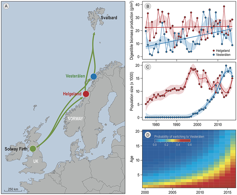
Figure 1. Barnacle goose spring-staging sites. All panels are reproduced from Tombre et al. (2019). (A) is a map of the migratory route (green arrows), and the two staging sites in red and blue. The geese winter at the Solway Firth, and breed on Svalbard. (B) shows the annual estimated staging site quality at both staging sites, estimated as the sum of the daily digestible biomass growth of grass leaves during the staging period. The lines are linear regressions and the shaded areas delineate the 95% confidence interval of local regressions. Panel (C) shows the number of spring staging geese at the two sites as found by the same study. Lines are the trends estimated by local regression, the colored areas depict confidence intervals. (D) shows the probability of geese of particular ages (y-axis) in each year (x-axis) to switch from staging in Helgeland to staging in Vesterålen in the subsequent year, as obtained from resightings of individually marked geese.

Tombre et al. estimated from ring resightings of individually marked birds that ~62% of the increasing use of Vesterålen can be attributed to birds that switched from the traditional to the new staging site in subsequent years, suggesting that the choice of staging site might be partly determined by geese responding to the changes in resource availability. However, in a year-to-year comparison switching rates did not correlate with foraging conditions, neither in the current nor in the previous year. This suggests a lack of direct response to changes in food availability, and implies that optimal foraging models (e.g., Bauer et al., 2006; Klaassen et al., 2006) are unlikely to explain the observed dynamics in staging site choice. Furthermore, young birds exhibited higher switching rates than older birds (Figure 1D). This implies that age-dependent changes in decision-making, which may (partly) result from social processes, affected the observed changes in migratory behavior.

We reason that the observed dynamics in staging site choice may be better understood when explicitly taking into account the ecological and social information that is available to individual animals, and the “decision rules” by which they integrate this information. To this end, we designed a set of simulation models, in which we implemented different potential sets of decision rules by which each individual in a simulated population of barnacle geese decides whether it stages in Helgeland or in Vesterålen. We used individual-based models, which are particularly suitable when the decisions by individuals and interactions between individuals are expected to affect the dynamics of the population (Bauer and Klaassen, 2013). Specifically, we analyzed which set of decision rules best explains the observed changes in staging-site use, by comparing the performance of different models. Using Approximate Bayesian Computation (Beaumont, 2010), we simultaneously test which model is the most plausible given the empirical data, and estimate the values of the parameters in the selected model(s). Each model contains a different combination of the following five components: (i) adjusting choice to the expected quality of the current staging site, obtained by memorized individual experiences in previous year(s), (ii) comparing expected quality of the current staging site with expected quality of the alternative staging site, which is obtained through explorative behavior in previous year(s), (iii) leaving the choice to others by traveling in a group, (iv) reconsidering staging site choice at arrival in Helgeland, dependent on the current number of geese and/or grass cover, and (v) impact of age on any of the previous four processes.

Methods

Individual-Based Models

We simulated barnacle goose population dynamics in individual-based population models with discrete time steps of one year (see Figure 2 for a visual description). In each model, the simulation runs started in 1970 with a population of 3,000 individuals with randomly assigned sex (50% chance of either male or female) and age (the initial age distribution was derived from a pilot simulation). Each individual was also assigned an age at which to become available as a partner, determined by drawing randomly from the Poisson distribution + 1 and λ = 1.5. This specific distribution with a mean of 2.5 and a standard deviation of 1.2 matches the empirically observed distribution (mean = 2.5, SD = 1.1; Choudhury et al., 1996). At the start of each time step, partnerships were determined, with pairs randomly assigned between available individuals (i.e., at or above the age of first reproduction and unpaired) of the opposite sex. Individuals remained with the same partner in subsequent years, only becoming available again as a partner when the partner died (Black et al., 2014; in reality the annual chance of a pair to separate is 2%, which we chose to ignore). All unpaired birds and a randomly assigned bird within each pair then chose a staging site: either Helgeland or Vesterålen. During the first time step, all individuals were set to choose Helgeland. In later time steps, individuals could instead decide to visit Vesterålen (see section Staging Site Decision Rules). Subsequently, each paired female reproduced with probability b_{s, t}, where s is the visited staging site and t is the calendar year.

FIGURE 2

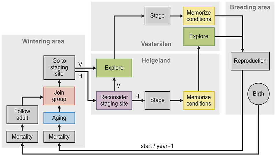
Figure 2. Flow chart diagram of the twelve individual-based models. Schematic overview of the individual-based model simulations. Each simulation begins with 3,000 individuals at start, and each individual follows the arrows in the diagram, with each cycle representing one year. The models, described in Table 2, differ only in the presence or absence of five components: “memory” (yellow), “reconsider” (purple), “exploration” (green), “groups” (red) and “aging” (blue). Mortality occurs with a probability of 0.11, reproduction occurs with a probability that depends on the conditions of the staging site (grass production as well as the number of geese at the staging site, see Equation 1) that the female has visited, being either Helgeland (H) or Vesterålen (V).

Previous simulation studies of goose behavior have focused on energetics (Bauer et al., 2006; Klaassen et al., 2006). While explicitly modeling density-dependent energy gain at staging sites and the consequences for reproductive success, they simplified the process of decision-making by assuming optimal behavior. We focused on the decision-making process and instead simplified the energetic part of the model. We assumed that b_{s, t} depends linearly on the annually estimated grass production at the staging site that she visited, and also decreases linearly with an increasing number of birds at that staging site, depending on the surface of foraging area:

$\begin{array}{ll}{b}_{s,t}=r_{s,t}\left(1-\frac{N_{s,t}}{K_s}\right),& (1)\end{array}$

where N_{s, t} is the abundance of birds at the visited staging site and K_s is the total surface area of suitable foraging habitat at that staging site (m²). The probability of reproduction in absence of competition, r_{s, t}, is a linear function of the digestible grass production per m² during the staging period in year t at staging site s, q_{s, t} (measured in g/m², see next section):

$\begin{array}{ll}{r}_{s,t}=0.1+a·q_{s,t},& (2)\end{array}$

where a is a conversion factor (m²/g). The lower boundary of 0.1 reflects the low probability of reproduction observed for geese with very low body condition before departing Helgeland (Prop et al., 2003). Instead of deriving K_H (carrying capacity in Helgeland) and conversion factor a mechanistically, we fitted them by performing model simulations without staging site choice, assuming all individuals to stage in Helgeland. The simulated population sizes were compared to the population count data between 1970 and 1997, when virtually all individuals visited Helgeland (see Figure 1). K_H and a were estimated as 44,000 and 0.0082, respectively, by selecting the values that minimized the distance between the simulated population sizes and the empirically derived values (see section Calculating the Distance of Each Simulation to Empirical Data). Based on the ratio of agricultural land in the two areas (summed surface of agricultural land in 2017 was estimated at 27.6 and 88.5 km² for the main goose areas in Helgeland and Vesterålen; data downloaded from www.ssb.no), and given that barnacle geese in Helgeland also make use of natural salt marshes and that barnacle geese in Vesterålen face competition for food with pink-footed geese (Tombre et al., 2019), we estimated conservatively that K_V was two times K_H. A higher value of K_V had no strong effect on the model selection results, as the population in Vesterålen remained far below carrying capacity in all simulations (see Appendix I and Table S1).

The number of offspring produced by a reproducing female was drawn from a Poisson distribution + 1 with λ = 1, resulting in a mean of two offspring, which equals the distribution in the number of juveniles associated with successful breeders in the wintering area (Black et al., 2014). At the end of each time step, individuals had a probability of dying, d, estimated at 0.11 (Black et al., 2014). Each simulation consisted of 48 time steps, representing the period from 1970 to 2017.

Grass Production at the Staging Sites

The digestible grass production per m² during each spring staging period t at staging site s, q_{s, t} (g/m²), was taken from Tombre et al. (2019). It was estimated as the sum of the daily digestible biomass growth of grass leaves from 30 April to 20 May (Prop and Black, 1998). The daily values were calculated by means of the simulation model CATIMO (Canadian Timothy Model; Bonesmo and Bélanger, 2002a,b). CATIMO simulates the daily growth of cell walls and cell contents in the leaves of timothy, Phleum pratense. Timothy is one of the main agricultural grass species and an important food source for barnacle geese in Norway (Black et al., 1991). Daily grass growth (g/m²) was converted to digestible daily grass growth (g/m²) by taking into account that the digestible proportion for barnacle geese is 0.16 and 0.64 for cell wall and cell content respectively (Prop and Vulink, 1992). The simulations were based on daily local temperature and radiation values. See Tombre et al. (2019) for a full explanation.

Staging Site Decision Rules

We compared 22 models, all with different decision rules determining the choice of staging site. Each set of decision rules is a combination of five components. The first component is memory, which we incorporated as an effect of staging site quality that the focal individual experienced in previous years. The second component is exploration, which we modeled as an effect of staging site quality at the alternative staging site in previous years when the individual was alive. The third component is traveling in groups. This is an effect of the staging site choice of others, in most cases the group leader, and hence a consequence of social learning. The fourth component is to reconsider staging site choice at arrival in Helgeland, with each individual continuing migration to Vesterålen with a probability that depends on the number of geese in Helgeland and/or the grass cover in Helgeland. As the fifth component, we included age-dependent differences between individuals in any of the four previous components (see also Figure 2).

In all models, paired birds stay together and normally return to the staging site of the previous year. In case newly paired birds did not visit the same staging site in the previous year, they make a random choice between both staging sites. Analysis of ring resightings before and after pair formation does not suggest a sex bias (TO and JP, unpublished data). Unpaired birds normally visit the staging site of the previous year. We assumed that each individual has an 18% probability of remaining with its parents during the first spring migration (Black et al., 2014), thereby copying the staging site choice of the parents. The first-year birds that do not stay with their parents follow others, based on one of the following criteria (denoted by parameter c_juv, for all parameters see Table 1): (1) follow a random non-first-year bird, (2) follow a parent (i.e., an individual that has produced offspring in the previous year), or (3) follow an individual of at least 10 years old, which is approximately the top 30% of the age-distribution (Black et al., 2014).

TABLE 1

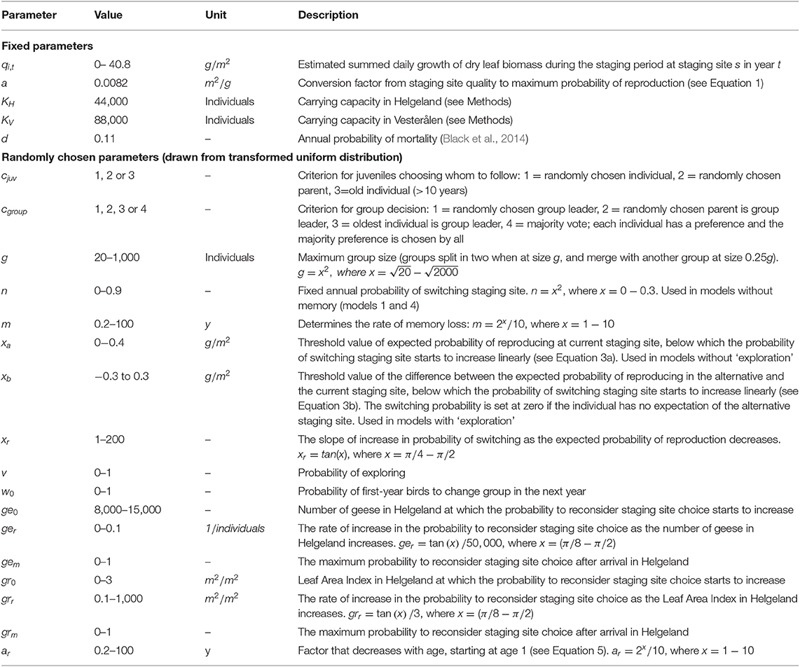
Table 1. Parameter values used in the simulation runs.

On top of this basic scheme, each individual can decide to switch staging site relative to the previous year. In the first model, each individual has a fixed annual probability of switching staging site (parameter n). Subsequent models incorporate different combinations of the five components as described below.

Memory

In each year, the expected probability of reproducing when returning to the current staging site (as opposed to switching to the other staging site), E(b_c), is given by a weighted average of its past experiences at that site. The weight of each of those experiences is given by the decay function $e^{-\frac{y}{m}}$, where y is the ‘age' of the experience (in years) and parameter m determines the rate at which memories fade. We assumed that individuals start switching to the other staging site when E(b_c) falls below a threshold that is given by parameter x_a. Below this threshold, the probability of switching increases with decreasing E(b_c)with a rate that is determined by parameter x_r, where:

$\begin{array}{ll}P\left(switch\right)=x_r\left(max\left(0,x_a-E\left(b_c\right)\right)\right).& (\mathrm{3a})\end{array}$

Exploration

Individuals explore the alternative staging site at the end of the staging period with probability (v), enabling them to inform their expectation of the reproduction probability when visiting the alternative staging site, E(b_a). If the difference between E(b_a) and E(b_c) is larger than x_b, then the probability of switching staging site in the next year is given by:

$\begin{array}{ll}P\left(switch\right)=x_r\left(max\left(0,x_b-E\left(b_c\right)+E\left(b_a\right)\right)\right),& (\mathrm{3b})\end{array}$

where parameter x_r determines how fast the probability of switching increases as the difference between E(b_a) and E(b_c) increases. This component only affects the model results when memory is also implemented, with equation 3b replacing 3a.

Groups

Instead of individually deciding where to go, birds may also choose to follow another individual, thereby copying its choice of staging site. We modeled this by assigning each bird to a group, and determining staging site choice per group instead of per individual. In this case, juveniles do not join an individual, but a group. We assumed that 18% of the juveniles joins the group of their parents (Black et al., 2014), and the rest joins a randomly chosen group. Group decisions may be made in different ways, denoted by parameter c_group. We assumed that individuals either (1) form groups with a single leader, which may be (1) a random bird, (2) a randomly chosen parent (i.e., an individual that has produced offspring in the previous year), or (3) a randomly chosen bird from among the oldest ones. Alternatively, each group member first makes an individual choice as explained above, after which the group reaches consensus by adopting the “majority vote” (4). Note that simple and plausible behavioral mechanisms allow individuals to follow any of these rules, without having an overview of the process (Couzin et al., 2005). We further assumed that individuals join the same group as in the previous year (but see component v, Aging). Maximum group size is determined by parameter g, with groups splitting into two equally sized groups when larger than g, and merging with a random other group when smaller than 0.25g.

Reconsidering Staging-Site Choice

At arrival in Helgeland, individuals have the possibility to reconsider their choice, and continue to Vesterålen. The probability to continue is either linearly dependent on the number of geese, N_H (Reconsider_geese), or on the grass cover at arrival in Helgeland (Reconsider_grass). Grass cover is calculated for each day in CATIMO as the leaf area index, LAI, measured in m² of grass leaves per m² of ground. Both functions depend on three parameters: the number of geese or the grass cover at which the probability to switch starts to increase (ge₀ and gr₀), the linear rate at which the probability increases (ge_r and gr_r), and the maximum switching probability (ge_m and gr_m):

$\begin{array}{ll}P\left(Reconside{r}_{geese}\right)=\left(max\left(0,min\left(g{e}_m,g{e}_r*(N_H-g{e}_0)\right)\right)\right)& (\mathrm{4a})\end{array}$

$\begin{array}{ll}P\left(Reconside{r}_{grass}\right)=\left(max\left(0,min\left(g{r}_m,g{r}_r*(LA{I}_H-g{r}_0)\right)\right)\right)& (\mathrm{4b})\end{array}$

Aging

We explored four different potential effects of age. The first assumed that the influence of previous experiences on the current decision decreases with the age of the individual. We modeled this by multiplying the probability of switching (see Equations 3a and 3b) with an age-factor a that changes with age according to the function

$\begin{array}{ll}a=e^{\frac{1-age}{a_r}},& (5)\end{array}$

where age is measured in years. Parameter a_r (also in years) determines the strength of the age-effect. A second possibility is that the probability of exploring (v) decreases with the individual's age, which is modeled by multiplying v by age-factor a. Thirdly, if the animals make migratory decisions in groups (see component i), then there may be an age-effect in the probability of changing to a randomly chosen new group, w₀, which is then multiplied by the age-factor a. Fourthly, there could be an age-effect in the tendency of individual geese to reconsider their staging site choice upon arrival in Helgeland. This is modeled by multiplying the probability to reconsider (Equations 4a and 4b) with the age-factor a.

Empirical Data

To determine which model is most plausible, we compared the simulations to two different sets of empirical data, both published by Tombre et al. (2019). The first set consists of the annual number of spring staging barnacle geese in Helgeland and in Vesterålen. This set contains 86 data points, being the estimated numbers of birds at each site in each year from 1975 to 2017 (Figure 1C). They were derived from annual counts during the staging period in Helgeland and Vesterålen, and annual counts of the total population size in the wintering area. The second set of data points consists of the probabilities of individual birds switching from staging in Helgeland to staging in Vesterålen in subsequent years (from here on referred to as “switching probabilities”). Each data point is the switching probability for an individual of a given age (age 1 to age 20) in a particular calendar year between 2000 and 2016 (Figure 1D). These data points were derived from resightings of marked individuals at both staging sites, as well as the wintering and the breeding area. Further details can be found in Tombre et al. (2019). As hardly any geese were observed staging in Vesterålen from 1975 to 1995, we infer that switching probabilities from Helgeland were zero from 1975 to 1995 for all ages. The years 1996 to 1999 were not part of the analysis. This resulted in a total of (21 + 17) × 20 = 760 data points. We did not compare the switching probabilities in the other direction (from Vesterålen to Helgeland), because these could not be estimated in years when the simulated bird numbers were zero in Vesterålen.

Model Selection: Approximate Bayesian Computation

We evaluated the relative strength of the different models by comparing simulations to the empirical data using Approximate Bayesian Computation (ABC; Beaumont, 2010) in R (R Core Team, 2018). This statistical tool has been developed to quantify the fit of different individual-based models to different sets of empirical data simultaneously. The ABC-method allows the fit of different models to be compared (e.g., models with and without memory), as well as comparing the fit of different parameter values within each model (e.g., values of a parameter determining the rate of memory loss). The method is called “Bayesian” because the method updates the degree of belief in each model given the empirical data. It is “Approximate” because it is not an analytical method, which is generally not an option for individual-based models, but instead relies on simulations (van der Vaart et al., 2015). We used rejection-ABC, the simplest and most accessible type of ABC that can be used for ecological models with multiple parameters (van der Vaart et al., 2015, 2016). Calculations were performed as in the R-package “abc” (Csilléry et al., 2012), except for indicated differences. Below, we explain the method step by step.

First, parameter values are defined. Where possible, parameters were estimated from the literature (see Table 1). For the other parameters, distributions were defined such that all possible values are included (see Table 1). These distributions are referred to as “prior distributions.” Then, 10,000 simulation runs were performed for each model. For each simulation, the values of all parameters in the model were drawn at random from the prior distributions. After all simulation runs were performed, we calculated the distance between each run and the empirical data (see next section). To give equal weight to both used datasets (bird numbers and switching probabilities), we calculated the distance of each simulation run to the empirical data separately for each dataset, and then took the mean of the two to arrive at a single distance estimate for each simulation run. Finally, the 100 runs with the smallest distance were selected. The evidence for model x relative to model y is expressed by the Bayes factor (B_{x, y}), which in this context is defined as the ratio of simulations from each model among the selected runs (van der Vaart et al., 2016).

To test whether the result would change with more simulations, we ran a bootstrapping test of the model selection accuracy by repeating the procedure 100 times, each time with a randomly chosen half of all simulation runs. To evaluate the ability of the ABC-method to distinguish between different models, we carried out cross-validation as implemented in the function “cv4postpr” in the “abc” R-package, and described in Csilléry et al. (2012). First, 100 simulation runs are randomly selected from each model. Then, for each of these runs, the complete model selection procedure is repeated after removing this run from the simulation data and replacing the empirical data with this run. The result is a “confusion matrix”, where each row represents the number of simulations under each model, and each column represents the number of simulations assigned to that model by the model selection procedure.

The distribution of parameter values among the selected simulation runs (“posterior distributions”) can be regarded as a probability distribution for each parameter, and acts as a sensitivity analysis. To test whether the posterior distributions were significantly different from the prior distributions (distribution of parameter values among all runs), we performed a Chi-square test after dividing the data into 10 equally-sized bins with the function “bin” in R-package OneR (von Jouanne-Diedrich, 2017). To correct for multiple testing, we applied a Bonferroni correction to the standard significance level of 0.05.

Calculating the Distance of Each Simulation to Empirical Data

Distance (ρ) is defined as the standardized Euclidian distance between all data points j in simulation i (M_i) and the same data points in the empirically derived data (D):

$\begin{array}{ll}\rho (M_i,D)=\sqrt{{\displaystyle \sum _j}{\left(\frac{M_{ij}-D_j}{sd\left(M_j\right)}\right)}^2},& (6)\end{array}$

where M_{i, j} is the output of run i for datapoint j, D_j is the empirically derived value of data point j, and sd(M_j) is the standard deviation of data point t in all simulation runs. As in van der Vaart et al. (2015), we used standard deviation instead of median absolute deviation (as is done in the “abc” package; Csilléry et al., 2012), because the median was zero for several datapoints and this led to undefined distances. To avoid overfitting, we chose to compare the simulations to the statistically estimated trends (Figures 1B,C), rather than to the raw empirical data. We made this decision because an unknown part of the inter-annual variation in the empirical data is caused by non-modeled processes, such as annual conditions in the breeding area and observation errors.

Reducing the Number of Simulations

To reduce the required number of simulation runs, we adopted a two-step model selection procedure. First, we performed a model selection of scenarios without the “age” component (models 1 to 15 in Table 2), and executing 10,000 simulation runs per model. We then composed seven additional models based on the selected models, but also including an age-effect (models 16 to 24 in Table 2), and executed 10,000 simulations per model. We did not consider models with an age-effect on more than one component, to further limit the number of models to be tested. These additional models were tested in a new model selection procedure, also including the selected models from the first model selection. For parameters in the first selection where the posterior distribution was significantly different from the prior distribution (Figure S1, Table 3), we updated the prior distributions for the simulations in the second model selection procedure (Table 3).

TABLE 2

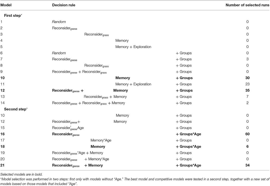
Table 2. Model selection results, showing for each model the number of runs among the best 100 simulation runs.

TABLE 3

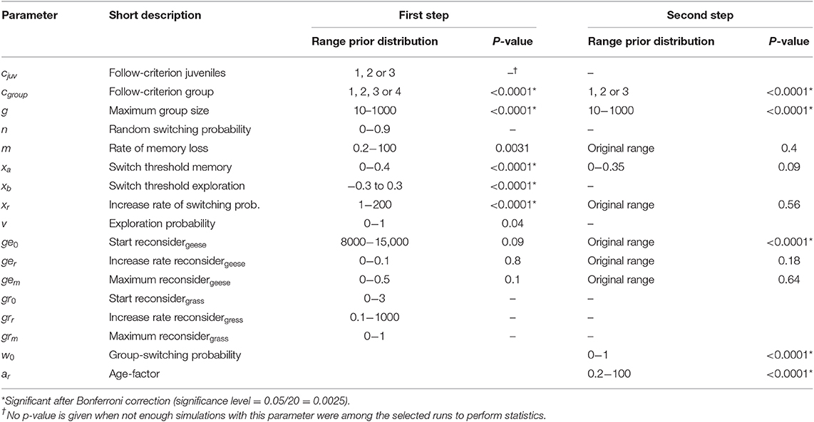
Table 3. Significance test of parameter distributions in selected simulations.

Results

Model Selection

The simulation most similar to the empirical data was produced by model 16, which includes “reconsider_geese”, “groups”, and an age-effect on “groups.” The pattern resulting from this simulation corresponded to the observed annual bird numbers at both staging sites (Figures 3D,E). Moreover, it showed a decrease in switching probability with age (Figure 3F), which was similar to the pattern in the empirical data (Figure 1D). This model was also the best represented model among the 100 best simulation runs (60 out of 100 runs, Table 2). The same model but with “memory” (model 21) was represented with 34 runs. With a Bayes factor of B_16,21 = 1.8 there is no evidence that memory does not play a role, but it does not improve the performance of the model in explaining the empirical data. Roughly, a Bayes factor of 3 to 10 is regarded as “substantial evidence” and above 10 as “strong evidence” (Kass and Raftery, 1995; van der Vaart et al., 2016). Apart from models 16 and 21, only model 18 (model 21 but without “reconsider_geese”) occurred among the 100 best models, with 6 runs (B_16,18 = 10 and B_21,18 = 5.7), meaning that there is substantial evidence for models 16 and 21 over model 18, and strong evidence over all other models. Hence, the results suggest that staging site choice is made in groups, with a decrease over age in the probability that individuals change groups, and that groups switch to another staging site based on the current number of geese at the staging site. The results are indefinite regarding the role of previous experiences at the alternative staging site. There is no evidence that exploration of the other staging site in previous years plays a role, nor that there is an effect of current food conditions at the staging site.

FIGURE 3

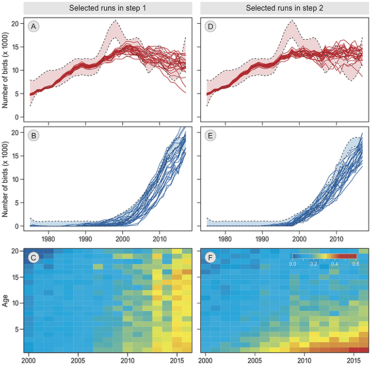
Figure 3. Patterns in best simulation runs. (A,B,D,E) show the annual numbers of barnacle geese staging in Helgeland and Vesterålen, respectively, from 1975 to 2017. The empirical estimates ± confidence interval (Tombre et al., 2019) are indicated by the light colors and dashed lines. Solid lines are the 25 best simulation runs. (C,F) shows for the single best simulation run the probability of switching from Helgeland to Vesterålen in the next year, by calendar year (2000–2016, x-axis) and by age (0–20, y-axis). The results of the first step in the model selection are on the left (A–C), the results of the second and final step are on the right (D,E,F).

Model Validation

Because models 16 and 21 both came out as likely to underlie the empirical data, we focused on these models in the model validation. When repeating the model selection analysis 1,000 times with a randomly chosen half of the data, models 16 and 21 together always made up the majority of the selected runs (range 91–100 out of 100 selected runs, mean 96, Figure 4). Hence, the evidence for models 16 and 21 relative to the others is robust. The only other model that appeared among the selected simulations was model 18 (“memory”, “groups” and an age-effect on groups, mean 4, range 0–9). The cross-validation procedure suggested that the model selection performs badly in estimating the underlying model of randomly drawn simulations: of the runs that were produced by model 16 or 21, only 67% were also estimated as such (Figure S2). This result was to be expected, because simulations were similar between models for a large proportion of parameter combinations. For example, switching did not occur at all in many simulation runs of all models with “groups” (between 6 and 40%). When performing the cross-validation procedure with the 100 best fitting runs of each model instead of randomly drawn runs, then 98.5% of the runs produced by model 16 or 21 were also estimated as such (Figure S2). Hence, when the data was close to the observed trends, the model selection performed well.

FIGURE 4

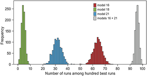
Figure 4. Bootstrapping test of model selection. The ABC-analysis was repeated 100 times, each time using a randomly drawn 50% of all simulation runs. Plotted are the frequency distributions of the representation of each model among the 100 best simulation runs in each repeat, excluding zero. The only models that always occurred among the selected runs are models 18 (green, mean = 4), 21 (blue, mean = 32) and 16 (red, mean = 64). Models 16 and 21 together always represented at least 91 of the 100 selected runs (gray, mean = 96). These are two models that include “reconsider_geese”, “grouping”, and an age-effect on “grouping.” Model 21 additionally includes “memory” (see Table 2 and Figure 2).

Parameter Estimation

In the 100 selected simulations runs of the first step in the model selection (see Figures 3A–C for simulation results), the distribution of values (posterior distributions) of 10 out of 15 parameters were significantly different from the defined prior distributions, of which five were in models that were represented among the best simulations (Table 3, Figure S1). For those parameters, we defined new prior distributions for use in the simulation runs for the main model selection (Table 3). In the selected simulations after the second step in the model selection, the posterior distributions of five out of ten parameters were significantly different from the defined prior distributions (c_group, g, ge₀, w₀ and a_r, Table 3, Figure 5).

FIGURE 5

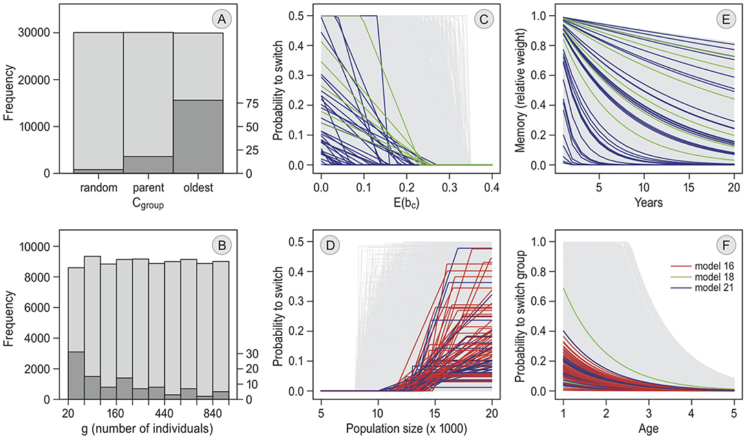
Figure 5. Parameter values of selected simulation runs. The pre-defined parameter distributions from which random values were drawn for each simulation are given in light gray. The frequency distributions of parameter values among the 100 selected simulation runs in the main model selection (see Table 2) are given in dark gray. In the line graphs, each model is shown in a different color. For the bar plots, patterns did not differ between models. (A) gives the following criterion in each simulation of the models with “groups” (parameter c_group). (B) is the frequency distribution of the maximum group size in each simulation run (parameter g). The lines in (C) define how the annual switching probability depends on the individual's expected probability of reproducing at the current staging site, E(b_c). They are determined by parameters x_a (threshold value below which the probability becomes non-zero) and x_r (the slope of the line below x_a) in the models with memory but without exploration. In (D), the lines are determined by parameters ge₀, ge_r and ge_m in the models with “reconsider_geese”, which determine how the probability to switch preference after arrival at the staging site, depending on the number of geese there. (E) shows how, resulting from differences in m, the weight of each memory declines over the years. The lines in (F) depend on parameters w₀ and a_r, and define how the probability of switching between groups decreases with age in each simulation (only models 16 and 21).

In all of the selected runs the birds traveled in groups. Smaller groups occurred more often among the selected runs than larger groups (see Figure 5B). In most of the selected runs, the oldest individuals led the group (78 out of 100 runs, Figure 5A). Simulations where group decisions were made by a majority vote always performed badly (see Table 3 and Figure S1; it did not occur in the selected runs in the first step, and was therefore removed from the prior distribution of the main selection procedure). Individuals switched between groups in all selected simulations, with most of the runs having an initial switching probability below 0.4, and a relatively slow decrease with increasing age (Figure 5F). In the selected runs where the probability for a group to switch increased with goose numbers at Helgeland (94 out of 100), birds started to switch when numbers were between 10,000 and 15,000 geese (parameter ge₀). The selected runs including “memory” and “reconsider_geese” responded less strongly to density (parameter ge_r) than the runs with “memory” but without “reconsider_geese” (Figure 5D). There was no pattern in the maximum probability to reconsider staging site (parameter ge_m; Figure 5D). The selected runs with memory (40 out of 100) showed no clear pattern in the rate of memory loss (parameter m; Figure 5F), suggesting that the rate of memory loss is not importantly affecting the dynamics. The same was the case for x_r, the rate at which the probability of switching increases when the expected probability of reproducing declines (the slopes in Figure 5C).

Discussion

Simulations resembled the empirical data best when geese were assumed to travel in small groups that are led by the oldest individuals, and when young geese switched more between groups in subsequent years than did older individuals (Table 2, Figure 5). Further, the results suggest that the current food conditions are of minor importance to staging site choice, but that the abundance of geese in Helgeland does increase the probability for groups to reconsider their choice and continue to Vesterålen. The model results are indecisive about whether experiences acquired by the group leaders in previous years, i.e., the “memory” component, influence the decision to switch staging site. We found no evidence that experiences at the alternative staging site in previous years contributes to the decision (Table 2). Below we discuss the implications of these results in more detail.

Grouping

The well-known fact that geese operate in groups need not inherently imply that each individual's choice of staging site is influenced by other members the group. For example, group-foraging pink-footed geese during spring staging decided individually on their specific daily foraging locations (Chudzinska et al., 2016). Our results are the first to suggest that group decisions do play a role in the choice of staging site. In all selected simulations (i.e., best fitting with the empirical data), staging site choice was made in groups.

The results further suggest that these decisions are not arrived at by a majority vote. The gradual increase in numbers in Vesterålen in the 1990s is not compatible with this decision rule, which requires a high proportion of all individuals to prefer switching, before the first geese start to switch. This aligns with the idea that strong conformity is generally not a good strategy in changing environments, because innovative behavior is unlikely to spread even when highly adaptive (Eriksson et al., 2007; Kandler and Laland, 2009). The most likely group decision rule was to follow the oldest, and therefore most experienced, bird of the group. This rule performed better than following parents (Chi-squared test, ${\chi }_1^2=36.6$, p < 0.0001), which in turn performed better than following a random individual (Chi-squared test, ${\chi }_1^2=7.7$, p = 0.006).

Following experienced birds might be adaptive because the annual food conditions at the staging site vary stochastically (Figure 1B), and longer experience will provide a better prediction of next year's staging site conditions. In contrast, following an individual that produced offspring in the previous year is hardly predictive of the chances to reproduce in this year if annual stochasticity is high (Baldini, 2012). This may explain why the model results indicated that following an individual that raised offspring was less likely than following an experienced leader. That following experienced birds is better than following successful breeders also could explain why in reality most first-year barnacle geese choose not to follow their parents on their first spring migration; on average, it would provide a higher pay-off to follow old and experienced individuals than to follow the parents. However, inclusive fitness arguments predict that unrelated group members may be more hostile than parents or other related individuals. Indeed, this also holds for barnacle geese (Black et al., 2014). Nonetheless, there are more examples of animals that are more likely to copy old (Amlacher and Dugatkin, 2005) and knowledgeable (Kendal et al., 2015) individuals, and to copy experienced others rather than the parents (Agostini et al., 2017). In bird flocks, leaders have been shown to be the more experienced individuals (Flack et al., 2012; Mueller et al., 2013). Our results imply that following experienced birds is especially advantageous when recent success needs not be a good predictor of subsequent success, but multiple-year averages of success are.

Reconsideration of Staging Site Choice at Arrival in Helgeland

The component “reconsider_geese” featured in all selected simulation runs. In models with this component, group leaders are more likely to reconsider their staging site choice after arrival in Helgeland in years when the number of birds in Helgeland is high. Simulations with this density-dependent effect corresponded better to the empirical data, because this effect keeps individuals from switching to Vesterålen before 1990. This also explains why simulation runs with “reconsider_grass” do not perform well, not even when combined with “reconsider_geese”. In models with “reconsider_grass”, the probability of reconsidering staging site choice increases as the grass phenology is more advanced at arrival in Helgeland. In those simulation runs, individuals do often colonize Vesterålen before 1990 because years with an early spring also occurred before 1990 (Figure 1B). Hence, these results suggest that the choice between Helgeland and Vesterålen is not a direct response to the “green wave” of spring phenology (van der Graaf et al., 2006). Instead, the growing preference for Vesterålen follows from a response to other geese, both positive (grouping) and negative (density-dependent switching).

Memory and Exploration

From an optimal foraging perspective, it is expected that any knowledge about the conditions at the current or alternative staging site should play a strong role in the decision whether or not to return to the current site in the following year (Stephens and Krebs, 1986, Abrahms et al., 2019). This influence was captured in the “memory” and “exploration” components of the model. The “memory” component was part of 40 out of 100 of the selected simulations (models 18 and 21; see Table 2), Although this is not evidence against memory playing a role, we conclude that there is no need to assume that geese memorized foraging conditions at the staging site in the previous year(s). Note that this only concerns memory of foraging conditions. In all models, individuals (or at least group leaders) are assumed to have spatial memory, and remember the migration route and staging site of the previous year (Mettke-Hofmann and Gwinner, 2003).

Adding the “exploration” component also did not improve the fit of simulations to the data, as the best model in the first step of the model selection with exploration (model 12) was less well represented than the same model without exploration (model 11). Hence, the current results are also indecisive with regard to the importance of exploration for decision-making. Geese have only rarely been observed to spend a significant amount of time at both staging sites in one spring, but they occasionally made a short stop in Helgeland before continuing to Vesterålen (PS, IT and JP, unpublished data). Less frequently, geese staging in Helgeland were also observed in Vesterålen at the end of the staging period, although most geese fly directly north after staging in Helgeland (PS and Larry Griffin, unpublished visual observations of departing geese and satellite tracks). A potential way forward is to add a third set of empirical data to the comparison, for example containing information on individuals that were (or were not) observed at multiple staging sites, in relation to their switching behavior. However, exploring individuals may be easily missed by observers if they land only shortly or not at all, making it hard to determine the rate of occurrence by ring resightings. More information on the rate of exploration and age-dependent changes in exploration could be derived by tracking individuals with gps-tags. Another possibility is to model the effect of exploration in more detail, which might lead to a better fit with the current empirical data. For example, new simulations could allow the probability of exploring Helgeland when staging in Vesterålen to be different from the probability of exploring Vesterålen when staging in Helgeland.

Aging

The finding that migratory decisions are age-dependent confirms a general trend that young birds become more consistent in their migratory decisions as they grow older (Lok et al., 2011; Oppel et al., 2015; Vansteelant et al., 2017). In Eurasian spoonbills (Lok et al., 2011) as well as in pink-footed geese (Clausen et al., 2018), a higher probability for young individuals to switch wintering site between years was attributed to young birds being more explorative. This has also been the main hypothesis to explain the higher probability of staging site switching by barnacle geese (Tombre et al., 2019). However, our results suggest that juveniles do not explore new staging sites deliberately. Instead, they are more likely to travel with different groups in subsequent years, which results in a higher probability of ending up at different staging sites. Also this group-switching behavior might be understood as being “explorative”, but it is social exploration rather than spatial exploration. This is an important distinction because it implies that migratory innovation needs not start with young and naïve individuals, as was suggested before. The modeling exercise indicates that the colonization of Vesterålen is more likely to have been initiated by old and experienced individuals, which were being followed by young animals.

Suggestions for Future Research

By comparing our simulations to the statistical trends in the empirical data (instead of the raw empirical data) uncertainty in the empirical trends were not conveyed to the statistics of our model selection procedure. We think that this method is to be preferred over using the raw data in this case, because the empirical trends were derived from a resighting analysis of individual bird observations. That analysis takes into account the probability of either not observing a bird when it is actually there (resighting probability) or not observing a birds because it is dead (mortality probability; for details see Tombre et al., 2019). To take these considerations into account when comparing individual-based models to the raw data, it would be necessary to also simulate the process of data collection within these models. We propose that incorporating data collection in the simulation exercise could be an interesting venue for future research.

In individual-based models, each decision must be modeled explicitly (Bauer and Klaassen, 2013). The advantage is that all of the underlying assumptions, many of which remain implicit and are often ignored in other types of modeling, become explicit. A disadvantage is that it remains unknown how much the way a process is modeled affects the results. For example, we modeled the process of pair formation and group formation in a basic way, with young individuals choosing a partner or a group at random. There are indications that individuals will be more likely to group with others that they grew up with (Choudhury and Black, 1994; van der Jeugd et al., 2002). Other studies have shown that social structure within groups can have strong effects on group dynamics (e.g., Bateman et al., 2013). Modeling these aspects more precisely could produce further insights into the causes and consequences of group formation by barnacle geese.

We stress that we only investigated the tip of the iceberg when it comes to individual differences. There may well be differences in decision-rules between individuals other than those mediated by age. Research on individual differences (Dingemanse et al., 2010), including those in barnacle geese (Kurvers et al., 2009), has shown that animals within the same population and of the same age can differ greatly in personality characteristics such as dominance, aggression, and exploration. Although beyond the scope of this study, such individual variation could be incorporated as an extension of the current study by assuming that individuals within the same population can act according to different sets of decision rules.

Cultural Evolution of Migratory Behavior

Social learning is an essential part of migratory inheritance and development for many migratory bird species (Sutherland, 1998; Helm et al., 2006; Németh and Moore, 2014), and for barnacle geese in particular (e.g., Eichhorn et al., 2009; Jonker et al., 2013). This study is the first attempt to infer the details of the learning processes in migratory decision-making from empirical data. The results indicate that geese travel in groups led by the oldest individual whose decisions are density-dependent, and the modeling explains how barnacle geese are able to respond so rapidly to long-term trends in competition and climate change at the staging sites. This is in line with the long-held conviction that cultural evolution allows for faster adaptation than genetic evolution (Boyd and Richerson, 1985; Sutherland, 1998). However, copying the behavior of conspecifics can also inhibit behavioral adjustment, and cause sub-optimal traditions to be maintained (Warner, 1988; Day et al., 2001; Németh and Moore, 2014). In order for social learning to lead to rapid adaptation, it typically needs to be combined with some low amount of individual learning, or other processes that introduce variation (Rendell et al., 2010). Intriguingly, the decision process that we identified here as being the most likely for migratory decisions by barnacle geese, does exactly this. Most geese follow others, but some of the experienced geese that lead the groups alter their decisions in response to current conditions.

We have discussed how the adaptive value of the observed decision rules is expected to depend on the amount and nature of the environmental variation. Although we expect that our results will also apply to other decisions, both by barnacle geese and by other social species, we stress that care should be taken when generalizing the results. An interesting venue for future research will be to apply the methods presented here to other published studies of migratory behavior across taxa and across situations. Finding general patterns between decision rules and environmental and social context will help to understand why some populations are more vulnerable to environmental change than others, and allow for better predictions of the ecological consequences of climate change. Currently, most studies of population dynamics do not consider the specific processes by which animals make their decisions. While arguably in some cases this may be a legitimate simplification, in cases like the present one, social and developmental aspects of decision-making turn out to be essential for understanding the population-scale response to environmental change.

Data Availability Statement

All datasets generated for this study are included in the article/Supplementary Material.

Ethics Statement

Ethical review and approval was not required for the animal study because all the data for this study has been published elsewhere, and where necessary were approved by an Animal Ethics Committee.

Author Contributions

TO, JP, KL, and GR conceived the study design. JP, IT, and PS provided the data. TO performed the analyses and wrote the manuscript with contributions from all authors.

Funding

This research was funded by a grant from the Netherlands Organization for Scientific Research awarded to TO (ref 019.172EN.011).

Conflict of Interest

The authors declare that the research was conducted in the absence of any commercial or financial relationships that could be construed as a potential conflict of interest.

Acknowledgments

The manuscript benefitted from comments on an earlier draft by Magda Chudzinska, and from advice by Luke Rendell. We thank the two reviewers for their helpful comments, and Dick Visser for editing the figures. Although this is a theoretical study, it fully depends on the data published by Tombre et al. (2019). This data was painstakingly gathered by a large international team of observers to which we are indebted.

Supplementary Material

The Supplementary Material for this article can be found online at: https://www.frontiersin.org/articles/10.3389/fevo.2019.00502/full#supplementary-material

References

Abrahms, B., Hazen, E. L., Aikens, E. O., Savoca, M. S., Goldbogen, J. A., Bograd, S. J., et al. (2019). Memory and resource tracking drive blue whale migrations. Proc. Natl. Acad. Sci. U. S. A. 116, 5582–5587. doi: 10.1073/pnas.1819031116

PubMed Abstract | CrossRef Full Text | Google Scholar

Agostini, N., Baghino, L., Vansteelant, W. M. G., and Panuccio, M. (2017). Age-related timing of short-toed snake eagle Circaetus gallicus migration along detoured and direct flyways. Bird Study 64, 37–44. doi: 10.1080/00063657.2016.1264362

CrossRef Full Text | Google Scholar

Amlacher, J., and Dugatkin, L. A. (2005). Preference for older over younger models during mate-choice copying in young guppies. Ethol. Ecol. Evol. 17, 161–169. doi: 10.1080/08927014.2005.9522605

CrossRef Full Text | Google Scholar

Baldini, R. (2012). Success-biased social learning: cultural and evolutionary dynamics. Theor. Popul. Biol. 82, 222–228. doi: 10.1016/j.tpb.2012.06.005

PubMed Abstract | CrossRef Full Text | Google Scholar

Bateman, A. W., Ozgul, A., Nielsen, J. F., Coulson, T., and Clutton-Brock, T. H. (2013), Social structure mediates environmental effects on group size in an obligate cooperative breeder, Suricata suricatta. Ecology 94, 587–597. doi: 10.1890/11-2122.1

PubMed Abstract | CrossRef Full Text | Google Scholar

Bauer, S., and Klaassen, M. (2013). Mechanistic models of animal migration behaviour - their diversity, structure and use. J. Anim. Ecol. 82, 498–508 doi: 10.1111/1365-2656.12054

PubMed Abstract | CrossRef Full Text | Google Scholar

Bauer, S., Madsen, J., and Klaassen, M. (2006). Intake rates, stochasticity, or onset of spring: what aspects of food availability affect spring migration patterns in pink-footed geese anser brachyrhynchus? Ardea 94, 555–566.

Google Scholar

Bauer, S., Nolet, B. A., Giske, J., Chapman, J. W., Åkesson, S., Hedenström, A., et al. (2011). “Cues and decision rules in animal migration”, in Animal Migration – A Synthesis, eds E. J. Milner-Gulland, J. M. Fryxell and A. R. E. Sinclair (Oxford: Oxford University Press), 68–87. doi: 10.1093/acprof:oso/9780199568994.003.0006

CrossRef Full Text | Google Scholar

Beaumont, M. A. (2010). Approximate bayesian computation in evolution and ecology. Annu. Rev. Ecol. Evol. Syst. 41, 379–406. doi: 10.1146/annurev-ecolsys-102209-144621

CrossRef Full Text | Google Scholar

Berbert, J. M., and Fagan, W. F. (2012). How the interplay between individual spatial memory and landscape persistence can generate population distribution patterns. Ecol. Complex. 12, 1–12. doi: 10.1016/j.ecocom.2012.07.001

CrossRef Full Text | Google Scholar

Black, J. M., Deerenberg, C., and Owen, M. (1991). Foraging behaviour and site selection of barnacle geese Branta leucopsis in a traditional and newly colonized spring staging habitat. Ardea 79, 349–358.

Google Scholar

Black, J. M., Prop, J., and Larsson, K. (2014). The Barnacle Goose. London: T & AD Poyser/Bloomsbury.

Google Scholar

Bonesmo, H., and Bélanger, G. (2002a). Timothy yield and nutritive value by the CATIMO model: I. Growth and nitrogen. Agron. J. 94, 337–345. doi: 10.2134/agronj2002.0337

CrossRef Full Text | Google Scholar

Bonesmo, H., and Bélanger, G. (2002b). Timothy yield and nutritive value by the CATIMO model: II. Digestibility and fiber. Agron. J. 94, 345–350. doi: 10.2134/agronj2002.0345

CrossRef Full Text | Google Scholar

Boyd, R., and Richerson, P. J. (1985). Culture and the Evolutionary Process. Chicago, IL: University of Chicago Press.

Google Scholar

Budaev, S., Jørgensen, C., Mangel, M., Eliassen, S., and Giske, J. (2019). Decision-making from the animal perspective: bridging ecology and subjective cognition. Front. Ecol. Evol. 7:164. doi: 10.3389/fevo.2019.00164

CrossRef Full Text | Google Scholar

Choudhury, S., and Black, J. M. (1994). Barnacle geese preferentially pair with familiar associates from early life. Anim. Behav. 46, 747–757. doi: 10.1006/anbe.1993.1252

CrossRef Full Text | Google Scholar

Choudhury, S., Black, J. M., and Owen, M. (1996). Body size, fitness and compatibility in barnacle geese Branta leucopsis. Ibis 138, 700–709. doi: 10.1111/j.1474-919X.1996.tb04772.x

CrossRef Full Text | Google Scholar

Chudzinska, M., Ayllón, D., Madsen, J., and Nabe-Nielsen, J. (2016). Discriminating between possible foraging decisions using pattern-oriented modelling: the case of pink-footed geese in Mid-Norway during their spring migration. Ecol. Modell. 320, 299–315. doi: 10.1016/j.ecolmodel.2015.10.005

CrossRef Full Text | Google Scholar

Clausen, K. K., Madsen, J., Cottaar, F., Kuijken, E., and Verscheure, C. (2018). Highly dynamic wintering strategies in migratory geese: coping with environmental change. Glob. Chang. Biol. 24, 3214–3225. doi: 10.1111/gcb.14061

PubMed Abstract | CrossRef Full Text | Google Scholar

Couzin, I. D., Krause, J., Franks, N. R., and Levin, S. A. (2005). Effective leadership and decision-making in animal groups on the move. Nature 433, 513–516. doi: 10.1038/nature03236

PubMed Abstract | CrossRef Full Text | Google Scholar

Csilléry, K., François, O., and Blum, M. G. B. (2012). abc: an R package for approximate Bayesian computation (ABC). Methods Ecol. Evol. 3, 475–479. doi: 10.1111/j.2041-210X.2011.00179.x

CrossRef Full Text | Google Scholar

Dall, S. R. X., Giraldeau, L.-A., Olsson, O., McNamara, J. M., and Stephens, D. W. (2005). Information and its use by animals in evolutionary ecology. Trends Ecol. Evol. 20, 187–193. doi: 10.1016/j.tree.2005.01.010

PubMed Abstract | CrossRef Full Text | Google Scholar

Danchin, E., Giraldeau, L.-A., Valone, T. J., and Wagner, R. H. (2004). Public information: from nosy neighbors to cultural evolution. Science 305, 487–491. doi: 10.1126/science.1098254

PubMed Abstract | CrossRef Full Text | Google Scholar

Day, R. L., MacDonald, T., Brown, C., Laland, K. N., and Reader, S. M. (2001). Interactions between shoal size and conformity in guppy social foraging. Anim. Behav. 62, 917–925. doi: 10.1006/anbe.2001.1820

CrossRef Full Text | Google Scholar

Dingemanse, N. J., Kazem, A. J. N., Réale, D., and Wright, J. (2010). Behavioural reaction norms: animal personality meets individual plasticity. Trends Ecol. Evol. 25, 81–89. doi: 10.1016/j.tree.2009.07.013

PubMed Abstract | CrossRef Full Text | Google Scholar

Drent, R. H., Eichhorn, G., Flagstad, A., Van der Graaf, A. J., Litvin, K. E., and Stahl, J. (2007). Migratory connectivity in Arctic geese: spring stopovers are the weak links in meeting targets for breeding. J. Ornithol. 148, 501–514. doi: 10.1007/s10336-007-0223-4

CrossRef Full Text | Google Scholar

Eichhorn, G., Drent, R. H., Stahl, J., Leito, A., and Alerstam, T. (2009). Skipping the Baltic: the emergence of a dichotomy of alternative spring migration strategies in Russian barnacle geese. J. Anim. Ecol. 78, 63–72. doi: 10.1111/j.1365-2656.2008.01485.x

PubMed Abstract | CrossRef Full Text | Google Scholar

Eriksson, K., Enquist, M., and Ghirlanda, S. (2007). Critical points in current theory of conformist social learning. J. Evol. Psychol. 5, 67–87. doi: 10.1556/JEP.2007.1009

CrossRef Full Text | Google Scholar

Flack, A., Pettit, B., Freeman, R., Guilford, T., and Biro, D. (2012). What are leaders made of? The role of individual experience in determining leader–follower relations in homing pigeons. Anim. Behav. 83, 703–709. doi: 10.1016/j.anbehav.2011.12.018

CrossRef Full Text | Google Scholar

Guttal, V., and Couzin, I. D. (2010). Social interactions, information use, and the evolution of collective migration. Proc. Natl. Acad. Sci. U. S. A. 107, 16172–16177. doi: 10.1073/pnas.1006874107

CrossRef Full Text | Google Scholar

Helm, B., Piersma, T., and van der Jeugd, H. (2006). Sociable schedules: interplay between avian seasonal and social behaviour. Anim. Behav. 72, 245–262. doi: 10.1016/j.anbehav.2005.12.007

CrossRef Full Text | Google Scholar

Hoppitt, W., and Laland, K. N. (2013). Social Learning: an Introduction to Mechanisms, Methods and Models. Princeton, NJ: Princeton University Press. doi: 10.1515/9781400846504

CrossRef Full Text | Google Scholar

Jesmer, B. R., Merkle, J. A., Goheen, J. R., Aikens, E. O., Beck, J. L., Courtemanch, A. B., et al. (2018). Is ungulate migration culturally transmitted? Evidence of social learning from translocated animals. Science 361, 1023–1025. doi: 10.1126/science.aat0985

PubMed Abstract | CrossRef Full Text | Google Scholar

Jonker, R. M., Kraus, R. H. S., Zhang, Q., van Hooft, P., Larsson, K., van der Jeugd, H. P., et al. (2013). Genetic consequences of breaking migratory traditions in barnacle geese Branta leucopsis. Mol. Ecol. 22, 5835–5847. doi: 10.1111/mec.12548

PubMed Abstract | CrossRef Full Text | Google Scholar

Kandler, A., and Laland, K. N. (2009). An investigation of the relationship between innovation and cultural diversity. Theor. Popul. Biol. 76, 59–67. doi: 10.1016/j.tpb.2009.04.004

PubMed Abstract | CrossRef Full Text | Google Scholar

Kass, R. E., and Raftery, A. E. (1995). Bayes factors. J. Am. Stat. Assoc. 90, 773–795. doi: 10.1080/01621459.1995.10476572

CrossRef Full Text | Google Scholar

Kendal, R., Hopper, L. M., Whiten, A., Brosnan, S. F., Lambeth, S. P., Schapiro, S. J., et al. (2015). Chimpanzees copy dominant and knowledgeable individuals: implications for cultural diversity. Evol. Hum. Behav. 36, 65–72. doi: 10.1016/j.evolhumbehav.2014.09.002

PubMed Abstract | CrossRef Full Text | Google Scholar

Klaassen, M., Bauer, S., Madsen, J., and Tombre, I. (2006). Modelling behavioural and fitness consequences of disturbance for geese along their spring flyway. J. Appl. Ecol. 43, 92–100. doi: 10.1111/j.1365-2664.2005.01109.x

CrossRef Full Text | Google Scholar

Kölzsch, A., Bauer, S., De Boer, R., Griffin, L., Cabot, D., Exo, K. M., et al. (2015). Forecasting spring from afar? Timing of migration and predictability of phenology along different migration routes of an avian herbivore. J. Anim. Ecol. 84, 272–283. doi: 10.1111/1365-2656.12281

PubMed Abstract | CrossRef Full Text | Google Scholar

Kurvers, R. H. J. M., Prins, H. H. T., van Wieren, S. E., van Oers, K., Nolet, B. A., and Ydenberg, R. C. (2009). The effect of personality on social foraging: shy barnacle geese scrounge more. Proc. Royal Soc. B Biol. Sci. 277, 601–608. doi: 10.1098/rspb.2009.1474

PubMed Abstract | CrossRef Full Text | Google Scholar

Lok, T., Overdijk, O., Tinbergen, J. M., and Piersma, T. (2011). The paradox of spoonbill migration: most birds travel to where survival rates are lowest. Anim. Behav. 82, 837–844. doi: 10.1016/j.anbehav.2011.07.019

CrossRef Full Text | Google Scholar

Mettke-Hofmann, C., and Gwinner, E. (2003). Long-term memory for a life on the move. Proc. Natl. Acad. Sci. U.S.A. 100, 5863–5866. doi: 10.1073/pnas.1037505100

PubMed Abstract | CrossRef Full Text | Google Scholar

Mettke-Hofmann, C., Winkler, H., and Leisler, B. (2002). The significance of ecological factors for exploration and neophobia in parrots. Ethology 108, 249–272. doi: 10.1046/j.1439-0310.2002.00773.x

CrossRef Full Text | Google Scholar

Mueller, T., O'Hara, R. B., Converse, S. J., Urbanek, R. P., and Fagan, W. F. (2013). Social learning of migratory performance. Science 341, 999–1002. doi: 10.1126/science.1237139

PubMed Abstract | CrossRef Full Text | Google Scholar

Németh, Z., and Moore, F. R. (2014). Information acquisition during migration: a social perspective Auk 131, 186–194. doi: 10.1642/AUK-13-195.1

CrossRef Full Text | Google Scholar

Oppel, S., Dobrev, V., Arkumarev, V., Saravia, V., Bounas, A., Kret, E., et al. (2015). High juvenile mortality during migration in a declining population of a long-distance migratory raptor. Ibis 157, 545–557. doi: 10.1111/ibi.12258

CrossRef Full Text | Google Scholar

Prop, J., and Black, J. M. (1998). Food intake, body reserves and reproductive success of barnacle geese Branta leucopsis staging in different habitats. Nor. Polarinstitutt Skrifter 200, 175–193.

Google Scholar

Prop, J., Black, J. M., and Shimmings, P. (2003). Travel schedules to the high arctic: barnacle geese trade-off the timing of migration with accumulation of fat deposits. Oikos 103, 403–414. doi: 10.1034/j.1600-0706.2003.12042.x

CrossRef Full Text | Google Scholar

Prop, J., and Vulink, T. (1992). Digestion by barnacle geese in the annual cycle: the interplay between retention time and food quality. Funct. Ecol. 6, 180–189. doi: 10.2307/2389753

CrossRef Full Text | Google Scholar

R Core Team (2018). A Language and Environment for Statistical Computing“. Vienna: R Foundation for Statistical Computing. Available online at: https://www.R-project.org/ (accessed January 10, 2019).

Google Scholar

Rendell, L., Boyd, R., Cownden, D., Enquist, M., Eriksson, K., Feldman, M. W., et al. (2010). Why copy others? Insights from the social learning strategies tournament. Science 328, 208–213. doi: 10.1126/science.1184719

PubMed Abstract | CrossRef Full Text | Google Scholar

Sasaki, T., and Biro, D. (2017). Cumulative culture can emerge from collective intelligence in animal groups. Nat. Commun. 8:15049. doi: 10.1038/ncomms15049

PubMed Abstract | CrossRef Full Text | Google Scholar

Stephens, D. W., and Krebs, J. R. (1986). Foraging Theory. Princeton, NJ: Princeton University Press.

Google Scholar

Sutherland, W. J. (1998). Evidence for flexibility and constraint in migration systems. J. Avian Biol. 29, 441–446. doi: 10.2307/3677163

CrossRef Full Text | Google Scholar

Tebbich, S., Fessl, B., and Blomqvist, D. (2009). Exploration and ecology in Darwin's finches. Evol. Ecol. 23, 591–605. doi: 10.1007/s10682-008-9257-1

CrossRef Full Text | Google Scholar

Tombre, I. M., Oudman, T., Shimmings, P., Griffin, L., and Prop, J. (2019). Northward range expansion in spring-staging barnacle geese is a response to climate change and population growth, mediated by individual experience. Glob. Chang. Biol. 23, 3680–3693. doi: 10.1111/gcb.14793

CrossRef Full Text | Google Scholar

van der Graaf, A. J., Stahl, J., Klimkowska, A., Bakker, J. P., and Drent, R. H. (2006). Surfing on a green wave: how plant growth drives spring migration in the barnacle goose. Ardea 94, 567–577.

Google Scholar

van der Jeugd, H. P., van der Veen, I. T., and Larsson, K. (2002). Kin clustering in barnacle geese: familiarity or phenotype matching? Behav. Ecol. 13, 786–790. doi: 10.1093/beheco/13.6.786

CrossRef Full Text | Google Scholar

van der Vaart, E., Beaumont, M. A., Johnston, A. S. A., and Sibly, R. M. (2015). Calibration and evaluation of individual-based models using approximate bayesian computation. Ecol. Modell. 312, 182–190. doi: 10.1016/j.ecolmodel.2015.05.020

CrossRef Full Text | Google Scholar

van der Vaart, E., Johnston, A. S. A., and Sibly, R. M. (2016). Predicting how many animals will be where: how to build, calibrate and evaluate individual-based models. Ecol. Modell. 326, 113–123. doi: 10.1016/j.ecolmodel.2015.08.012

CrossRef Full Text | Google Scholar

Vansteelant, W. M. G., Kekkonen, J., and Byholm, P. (2017). Wind conditions and geography shape the first outbound migration of juvenile honey buzzards and their distribution across sub-Saharan Africa. Proc. Royal Soc. B Biol. Sci. 284:20170387. doi: 10.1098/rspb.2017.0387

PubMed Abstract | CrossRef Full Text | Google Scholar

von Jouanne-Diedrich, H. (2017). OneR: One Rule Machine Learning Classification Algorithm with Enhancements. R package version 2.2. Available online at: https://CRAN.R-project.org/package=OneR (accessed January 10, 2019).

Google Scholar

Warner, R. R. (1988). Traditionality of mating-site preferences in a coral reef fish. Nature 335, 719–721. doi: 10.1038/335719a0

CrossRef Full Text | Google Scholar