Robust Cooperative Moving Path Following Control for Marine Robotic Vehicles

1. Introduction

The motion control problem for underactuated robotic vehicles is a relatively mature area of research, with important works addressing trajectory tracking and path following schemes. In the path following (PF) problem, the vehicle is tasked to follow a fixed geometric path without the need of satisfying explicit time constraints, in contrast to trajectory tracking. A series of results addressing the PF motion control problem were published, starting with the pioneering work in Samson (1992); Micaelli and Samson (1993), and Aguiar and Pascoal (2007) for the case of wheeled mobile robots, Encarnação et al. (2000); Belleter et al. (2016) and references therein for marine vehicles and Cichella et al. (2011); Xargay et al. (2013) for UAVs.

A generalization of the path following problem is termed the Moving Path Following (MPF) motion control problem, which consists of steering the robotic vehicle along an a priori specified geometric path expressed with respect to a moving target frame. This problem finds applications in source seeking, convoy protection, target tracking, surveillance and monitoring and also autonomous landing. For example, in target tracking applications in the maritime environment, it is desirable for the vehicles to perform different types of maneuvers. These maneuvers can be framed as specific paths to be followed around the tracked target, and often allow the vehicle to have the necessary flexibility to operate in a highly complex environment, which is constantly inducing disturbances into its body due to the presence of maritime currents, waves and hydrodynamic effects. Further, it is observed that the MPF problem retains the advantages of the classical path following schemes (Aguiar et al., 2005) such as faster convergence of the robot to the moving path, while allowing the target reference frame to move freely. The works in Oliveira and Encarnação (2013) and Oliveira et al. (2016) introduced the MPF control problem for tracking of ground targets using Unmanned Aerial Vehicles (UAVs) and later on, Oliveira et al. (2017) extended the solution to the 3D case. The proposed approach was suitable for robotic vehicles requiring a minimum positive forward speed, such as certain types of AUVs. In Jain et al. (2018b), a Lyapunov-based MPF control approach was presented for robotic vehicles without this restriction. Other control methods such as vector field method (Kapitanyuk et al., 2017) and nonlinear model predictive control (Jain et al., 2018c) have been proposed to solve the MPF problem. In contrast to the contributions of this paper, the salient features of the above reviewed literature are that they do not consider the external disturbances that depend on the operational environment, such as maritime currents, wind or rough terrain, that can affect the performance of the MPF controller. Further, they assume that the velocity of the target frame is known.

In path following literature, the problem of robustness has been addressed for example, in Dagci et al. (2003), where a cascade sliding mode controller for both kinematics and dynamics of a robotic vehicle was designed. In Aguiar and Pascoal (2002), a disturbance observer for constant unknown ocean currents was designed to solve the problem of dynamic positioning and way-point tracking of an underactuated AUV. Later on, the problem of robustness against parametric uncertainty in trajectory tracking and path following was also addressed in Aguiar and Hespanha (2007). More recently, in Zhang et al. (2014), a sliding mode technique combined with a predictive control strategy was developed to compensate for the impact of the hydrodynamic damping coupling on a 3D path following task for an Autonomous Underwater Vehicle (AUV). In Wang et al. (2016), a H_∞ robust controller for ground vehicles is proposed to achieve path following in the presence of disturbances caused by delays and data packet dropouts. All of the above schemes consider robustness for the path following problem. From the best of the authors knowledge, the only work concerning the problem of robustness in MPF literature is Reis et al. (2019), where sliding mode based controllers and a disturbance observer were designed to compensate external disturbances acting on the robotic vehicle.

A further extension of the MPF framework for multi-robot applications and formation control is the Cooperative Moving Path Following (CMPF) control problem, which consists in steering N vehicles along N paths defined with respect to a moving target while achieving some coordination objective. A special case of CMPF control, where the paths are fixed with respect to a given reference frame is the framework of Cooperative Path Following (CPF). As a recent example, the robustness problem in CPF literature was addressed in Gu et al. (2019), where two cooperative path following controllers using an Extended State Observer to estimate and compensate external disturbances in the kinetic level were proposed and validated experimentally using Autonomous Surface Vehicles (ASVs). In (Jain et al., 2018a), an event-based controller was explicitly designed to reduce the frequency of communication between the robotic vehicles. The control strategy effectively decomposes the control structure into two distinct layers. The first is responsible for the motion control of each individual vehicle, termed the PF controller. The second, termed the cooperative controller, is responsible for achieving coordination between the robots by using a consensus law. However, (Jain et al., 2018a) does not consider uncertainties and disturbances acting on the robotic vehicles. By decoupling the motion control layer from the cooperative control layer, one could use robust MPF controllers in the first layer to deal with the presence of certain types of disturbances acting on the vehicles, without affecting the formation control.

This paper extends the results obtained for the MPF controllers proposed by Reis et al. (2019) to the Cooperative MPF framework. Two MPF control strategies are proposed for the motion control layer, both using a known target pose and estimates of the target velocities. The first strategy employs a First Order Sliding Mode (FOSM) term to achieve robustness against bounded disturbances. The second strategy seeks to directly compensate the disturbance by computing an estimate of the disturbance using a disturbance observer. The cooperative layer consists of the consensus law proposed by Aguiar (2017). The stability of the proposed control laws is analyzed and it is shown that the origin of the path error is stable and converges to a small neighborhood around zero, even in the presence of bounded estimation errors on the target velocities and environmental disturbances. The design and theoretical results for the two variants of the proposed robust controllers are experimentally validated in a CMPF scenario using Autonomous Underwater Vehicles.

2. Problem Formulation

2.1. Kinematic Model for an Underactuated Vehicle

Consider an inertial frame of reference {I} and N robotic vehicles, each with its body frame {B_i} attached to its center of mass. Define the set of N robotic vehicles as ${I}=\left\{1,2,\dots ,N\right\}$. The kinematic model of the i-th vehicle moving in ℝⁿ with n = 2, 3 can be expressed by

$\begin{array}{l}{\dot{p}}_i(t)=R_i(t)v_i+d_{v,i}\\ {\dot{R}}_i(t)=R_i(t)S({\omega }_i+d_{\omega ,i})& (1)\end{array}$

where $p_i\in {ℝ}^n$ denotes the position of the i-th robot with respect to the frame {I}, $R_i\in {S}{O}(n)$ denotes the rotation matrix from the frame {B_i} to an inertial frame {I}, $v_i\in {ℝ}^n$ and ${\omega }_i\in {ℝ}^{n(n-1)/2}$ are the linear and angular velocities of the i-th vehicle with respect to its own body frame, S(ω_i) ∈ 𝔰𝔬(n) is the skew-symmetric matrix associated to the angular velocity ω_i.

Finally, $d_{v,i}\in {ℝ}^n$ and $d_{\omega ,i}\in {ℝ}^{n(n-1)/2}$ are kinematic disturbances acting on each robot. Many different factors can be the source of these disturbances, depending on the type of vehicle and the operational environment. Marine vehicles such as AUVs are affected by unknown sea conditions that can induce unwanted external velocities due to maritime currents, waves and wind. In the case of aerial vehicles, wind and internal dynamics can induce some unwanted disturbances in the kinematic model. In this work, we consider the problem of controlling an underactuated vehicle at the kinematic level, with the control signal defined as

$\begin{array}{ll}{u}_i=\left[\begin{array}{c}{v}_{f,i}\\ {\omega }_i\end{array}\right]& (2)\end{array}$

where the body linear velocity v_i is defined as $v_i={\left[v_{f,i}0\right]}^T$ (n = 2) or $v_i={\left[v_{f,i}00\right]}^T$ (n = 3). This is the case for vehicles where only the longitudinal velocity v_{f, i} ∈ ℝ and the body angular velocity ${\omega }_i\in {ℝ}^{n(n-1)/2}$ can be controlled, such as some types of AUVs. We assume that the vehicle has an inner-loop autopilot controller that is responsible to track the linear and angular velocity commands generated by the controller based on the kinematic model of the robotic vehicle. Imperfect tracking by the inner-loop autopilot controller can further contribute to the velocity disturbances acting on the vehicle, that can be lumped into the terms d_{v, i} and d_{ω, i}.

2.2. Cooperative Moving Path Following Problem

In the CMPF control problem, the vehicles must follow a priori specified paths expressed with respect to a moving target whose position can be accurately estimated, while also maintaining some coordination objective. Define the target frame {T} with its origin attached to the target center of mass. Then, the cooperative MPF problem can be divided in the following two sub-problems.

2.2.1. Moving Path Following Problem

Let $p_t(t)\in {ℝ}^n$ denote the position of the target with respect to the frame {I}, and $p_{d,i}^t({\gamma }_i)\in {ℝ}^n$ be the desired path for vehicle i, specified with respect to the frame {T} and parameterized by the path variable γ_i ∈ ℝ. As illustrated by Figure 1, for a given γ_i and time t, p_{d, i}(γ_i, t) and ${\stackrel{\bullet }{p}}_{d,i}({\gamma }_i,t)$ denote the position and velocity of the virtual reference point that must be followed by the i-th vehicle, with respect to the inertial frame {I}:

$\begin{array}{ll}{p}_{d,i}({\gamma }_i,t)=p_t+R_t{p}_{d,i}^t& (3)\end{array}$

$\begin{array}{ll}{\stackrel{\bullet }{p}}_{d,i}({\gamma }_i,t)=v_t+R_t\left(\nabla p_{d,i}^t{\stackrel{\bullet }{\gamma }}_i+S({\omega }_t)p_{d,i}^t\right)& (4)\end{array}$

where $R_t(t)\in {S}{O}(n)$ is the rotation matrix of frame {T} with respect to {I}, $v_t(t)\in {ℝ}^n$, ${\omega }_t(t)\in {ℝ}^{n(n-1)/2}$ are the linear and angular target velocities and ∇ ≡ ∂/∂γ_i is the derivative with respect to γ_i.

FIGURE 1

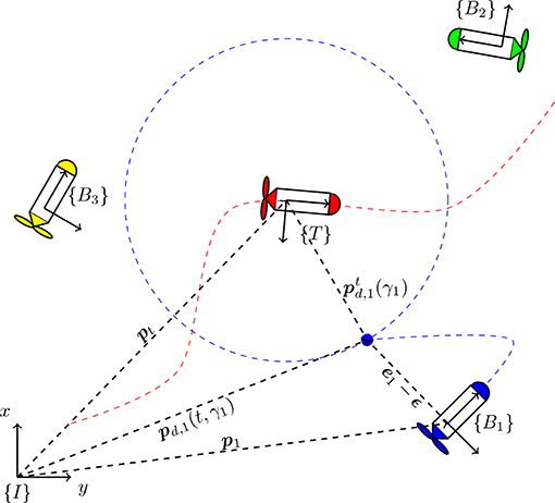
Figure 1. Coordinate frames and vector notation for N = 3 vehicles.

Assumption 2.1. The geometric path $p_{d,i}^t({\gamma }_i)$ is a differentiable function.

Note that Assumption 2.1 is already needed in order to compute (4) from (3). Suppose we wish to control the position of the nose of the i-th vehicle, or more generically, a point ${\bar{p}}_i=p_i+R_iϵ$ placed at a constant position $ϵ={\left[{ϵ}_1{ϵ}_2\right]}^T$ (n = 2) or $ϵ={\left[{ϵ}_1{ϵ}_2{ϵ}_3\right]}^T$ (n = 3) from the origin of {B_i}. Then, define the MPF error associated to the i-th vehicle as the vector

$\begin{array}{ll}{e}_i=R_i^T({\bar{p}}_i-p_{d,i}),i\in {I}& (5)\end{array}$

The objective of the MPF control problem is to design a control law u_i such that the origin e_i ≡ 0 is stable and e_i → 0 as t → ∞, $\forall i\in {I}$. That is, it is desired to steer the vehicles toward their moving geometric paths, such that ${\bar{p}}_i$ stabilizes around p_{d, i}(γ_i, t), $\forall i\in {I}$.

In order to control the progression of the virtual points p_{d, i}(t, γ_i) along the moving paths, the dynamics of the path variable ${\stackrel{\bullet }{\gamma }}_i$ should be explicitly controlled. This can be achieved by imposing the dynamics for γ_i as

$\begin{array}{ll}{\stackrel{\bullet }{\gamma }}_i=v_d+{\vartheta }_i,i\in {I}& (6)\end{array}$

where the scalar v_d is the desired nominal speed of the path variable and ϑ_i is a bounded control signal, designed to achieve CMPF objectives such as: (i) consensus over the path variables of the robotic vehicles to achieve a desired formation along the moving path and (ii) faster convergence to the moving path. To move along the geometric paths with the desired velocity, the vehicles must satisfy the desired speed assignments $|{\stackrel{\bullet }{\gamma }}_i-v_d|\to 0$ as t → ∞, $\forall i\in {I}$.

2.2.2. Cooperative Motion Control Problem

Assume that the i-th vehicle communicates with a fixed set ${{N}}_i\subset \mathbb{N}$ of neighbor vehicles. Given the path variables γ_i ($i\in {I}$) for the N vehicles and a given undirected, fixed communication topology among them, the objective of the cooperative motion control problem is to design a decentralized control law v_{r, i}(t) such that the positions of the virtual points are synchronized, that is, |γ_i − γ_j| converges to zero $\forall i,j\in {I}$ as t → ∞. To simultaneously achieve the speed assignment, coordination objective and also two other secondary objectives, function ϑ_i in (6) is decomposed as

$\begin{array}{ll}{\vartheta }_i=v_{r,i}(t)+g_{e,i}(t)+g_{\omega ,i}(t)& (7)\end{array}$

where v_{r, i}(t) is the cooperative control signal (to be designed) that is responsible for achieving consensus between the vehicles, while g_{e, i}(t) and g_{ω, i}(t) represent secondary objectives, where g_{e, i}(t) is an error correction term, responsible for delaying the evolution of the path variable in case of momentary vehicle failure, and g_{ω, i}(t) is a rotation correction term, responsible for canceling the rotational motion induced on the path by the rotation of the target. These functions are to be properly defined in section 3.3.

3. Robust Cooperative Moving Path Following Control

3.1. Robust MPF Controller Design

In this section, we consider the kinematic controller proposed in Jain et al. (2018a) with a modification designed to ensure robustness against disturbances. For the i-th vehicle, the error dynamics is given by

$\begin{array}{l}{\stackrel{\bullet }{e}}_i={\dot{R}}_i^T({\bar{p}}_i-p_{d,i})+R_i^T({\overline{\dot{p}}}_i-{\dot{p}}_{d,i}).\end{array}$

Using model (1) with control signal (2) and MPF error (5), the error dynamics can be rewritten as

$\begin{array}{l}{\stackrel{\bullet }{e}}_i=-S({\omega }_i+d_{\omega ,i})e_i+\Delta u_i+d_i-R_i^T{v}_t\\ -R_i^T{R}_t\left(\nabla p_{d,i}^t{\stackrel{\bullet }{\gamma }}_i+S({\omega }_t)p_{d,i}^t({\gamma }_i)\right)& (8)\end{array}$

where Δ is a constant matrix that can take the forms

$\Delta =\left[\begin{array}{cc}1& -{ϵ}_2\\ 0& {ϵ}_1\end{array}\right]\text{ or }\Delta =\left[\begin{array}{cccc}1& 0& {ϵ}_3& -{ϵ}_2\\ 0& -{ϵ}_3& 0& {ϵ}_1\\ 0& {ϵ}_2& -{ϵ}_1& 0\end{array}\right]$

for the planar (n = 2) and 3D (n = 3) cases, respectively. Note that it is always possible to choose ϵ such that Δ is full rank. Vector $d_i\in {\mathbf{\text{R}}}^n$ is the total external disturbance acting on the vehicle. In the planar case, it is given by

$\begin{array}{l}{d}_i=\left[\begin{array}{c}{R}_i^T{s}_{ϵ}\end{array}\right]\left[\begin{array}{c}{d}_{v,i}\\ d_{\omega ,i}\end{array}\right]\\ s_{ϵ}={\left[\begin{array}{c}-{ϵ}_2{ϵ}_1\end{array}\right]}^T& (9)\end{array}$

Remark 3.1. Notice that, by the triangle inequality, the total external disturbance d_i is bounded by ∥d_i∥ ≤ ∥d_{v, i}∥ + ∥d_{ω, i}∥∥ϵ∥.

Assumption 3.1. The total external disturbances d_i are bounded vector quantities.

Theorem 1 (Robust MPF). Consider an underactuated robotic vehicle described by (1) with control signal given by (2). Let the MPF error kinematics be described by (8), and consider that the pose of the i-th vehicle $\left\{p_i,R_i\right\}\in {ℝ}^n\times {S}{O}(n)$ and of the target frame $\left\{p_t,R_t\right\}\in {ℝ}^n\times {S}{O}(n)$ are known. Under Assumptions 2.1 and 2.2, the control law

$\begin{array}{l}{u}_i={\Delta }^{†}(-K_{p,i}{e}_i+R_i^T\left({\hat{v}}_t+R_{t}S({\hat{\omega }}_t)p_{d,i}^t\right)\\ +R_i^T{R}_t\nabla p_{d,i}^t{\stackrel{\bullet }{\gamma }}_i-w_i)& (10)\end{array}$

$\begin{array}{ll}{w}_i=\{\begin{array}{c}{\rho }_i\frac{e_i}{\parallel e_i\parallel },\parallel e_i\parallel \ge {ϵ}_w\\ {\rho }_i\frac{e_i}{{ϵ}_w},\parallel e_i\parallel <{ϵ}_w\end{array}& (11)\end{array}$

ensures that all trajectories of the MPF error are globally uniformly ultimately bounded and converge to a ball around the origin e_i = 0 that can be made arbitrarily small. In (10), the matrix Δ^† is the Moore-Penrose pseudo-inverse of Δ, $K_p\in {\mathit{\text{R}}}^{n\times n}$ is a positive-definite gain matrix and ${\hat{v}}_t\in {ℝ}^n$, ${\hat{\omega }}_t\in {ℝ}^{n(n-1)/2}$ are estimates of the target velocities. In (11), ρ_i is a scalar such that

$\begin{array}{ll}{\rho }_i\ge \parallel d_{v,i}\parallel +\parallel d_{\omega ,i}\parallel \parallel ϵ\parallel +\parallel {\tilde{v}}_t\parallel +\parallel {\tilde{\omega }}_t\times p_{d,i}^t({\gamma }_i)\parallel & (12)\end{array}$

where ${\tilde{v}}_t=v_t-{\hat{v}}_t$, ${\tilde{\omega }}_t={\omega }_t-{\hat{\omega }}_t$ are bounded estimation errors on the target velocities.

Proof. Define the Lyapunov candidate $V(e_i)=\frac{1}{2}{e}_i^T{e}_i$. Using the error dynamics in (8), its time derivative along the system trajectories is

$\begin{array}{ll}\stackrel{\bullet }{V}(e_i)=e_i^T(\Delta u_i+d_i-R_i^T{v}_t-R_i^T{R}_t\left(\nabla p_{d,i}^t{\stackrel{\bullet }{\gamma }}_i+S({\omega }_t)p_{d,i}^t\right))& (13)\end{array}$

where we have used the fact that $e_i^{T}S({\omega }_i+d_{\omega ,i})e_i=0$, since S(ω_i + d_{ω, i}) is skew-symmetric. Substituting control law (10) in (13) yields

$\begin{array}{ll}\stackrel{\bullet }{V}(e_i)=-e_i^T{K}_p{e}_i+e_i^T(D_i-w_i),& (14)\end{array}$

where $D_i=d_i-R_i^T\left({\tilde{v}}_t+R_{t}S({\tilde{\omega }}_t)p_{d,i}^t\right)$. Since K_p > 0, the first term is negative definite and bounded by $-{\lambda }_{\text{min}}(K_p){\Vert e_i\Vert }^2$. Next, we consider the two cases of (11), when ∥e_i∥ ≥ ϵ_w or ∥e_i∥ < ϵ_w.

• For ∥e_i∥ ≥ ϵ_w in (14), we have

$\begin{array}{l}\dot{V}(e_i)\le -{\lambda }_{\text{min}}(K_p){\Vert e_i\Vert }^2+e_i^T{D}_i-{\rho }_i\frac{e_i^T{e}_i}{\Vert e_i\Vert }\\ \le -{\lambda }_{\text{min}}(K_p){\Vert e_i\Vert }^2+\Vert e_i\Vert (\Vert D_i\Vert \text{}-\text{}{\rho }_i)\end{array}$

where the Cauchy-Schwarz inequality was employed on term $e_i^T{D}_i$. By Assumption 3.1, it is always possible to design ρ_i such that (12) is satisfied. Therefore, by Remark 3.1, choosing ρ_i ≥ ∥D_i∥ renders the second term on the right-hand side negative definite, which estabilishes that the trajectory e_i(t) of the closed-loop system reaches the ball ${B}({ϵ}_w):=\left\{e_i\in {ℝ}^n:\parallel e_i\parallel \le {ϵ}_w\right\}$ in finite time.

• When the trajectories are inside ${B}({ϵ}_w)$, we have ∥e_i∥ < ϵ_w, and (14) gets

$\begin{array}{l}\dot{V}(e_i)\le -{\lambda }_{\text{min}}(K_p){\Vert e_i\Vert }^2+e_i^T{D}_i-{\rho }_i\frac{e_i^T{e}_i}{{ϵ}_w}\\ \le -(1-\theta ){\lambda }_{\text{min}}(K_p){\Vert e_i\Vert }^2\\ -\left(\theta {\lambda }_{\text{min}}(K_p)+\frac{{\rho }_i}{{ϵ}_w}\right){\Vert e_i\Vert }^2+\Vert e_i\Vert \Vert D_i\Vert \end{array}$

where 0 < θ < 1. Then, using the inequality above, one can write:

$\begin{array}{l}\dot{V}(e_i)\le -(1-\theta ){\lambda }_{\min }(K_p){\Vert e_i\Vert }^2<0\forall \Vert e_i\Vert \ge {\mu }_i,\\ {\mu }_i=\frac{\Vert D_i\Vert {ϵ}_w}{{\lambda }_{\min }(K_p)\theta {ϵ}_w+{\rho }_i}\end{array}$

Note that μ_i ≤ ϵ_w for all 0 < θ < 1, which means that the trajectory of the closed-loop system e_i(t) again reaches the ball ${B}({\mu }_i)\subseteq {B}({ϵ}_w)$ in finite time.

This establishes that the trajectories are globally ultimately uniformly bounded, since $V=\frac{1}{2}{\Vert e_i\Vert }^2$ is radially unbounded (Khalil, 2002). Moreover, e_i(t) converges to the ball ${B}({\mu }_i)\subseteq {B}({ϵ}_w)$, which can be made arbitrarily small when ϵ_w → 0.      □

3.2. Robust MPF Controller Design With Disturbance Observer

In the presence of large amplitude disturbances, it may be difficult to tune the parameters ρ_i and ϵ_w so as to satisfy (12). In these situations, an observer can be designed to provide an estimate of the disturbance. Furthermore, this estimate can be used in the control law to compensate the real disturbance directly.

Without loss of generality, consider the planar problem. Consider that the vehicle pose $\left\{p_i,R_i\right\}\in {ℝ}^2\times {S}{O}(2)$ is known and that the vehicle orientation is parameterized by the planar angle ψ_i ∈ ℝ, such that $R_i=R_i({\psi }_i)\in {S}{O}(2)$.

Then, the disturbance observer for the translational disturbance is defined as

$\begin{array}{ll}\{\begin{array}{c}{\stackrel{\bullet }{\widehat{p}}}_i=R_i{v}_i+{\widehat{d}}_{v,i}+K_1{\tilde{p}}_i\hfill \\ {\stackrel{\bullet }{\widehat{d}}}_{v,i}=K_2{\tilde{p}}_i,\hfill \end{array}\hfill & (15)\end{array}$

where the estimation errors are defined as ${\tilde{p}}_i=p_i-{\widehat{p}}_i$ and ${\tilde{d}}_{v,i}=d_{v,i}-{\widehat{d}}_{v,i}$, and the positions p_i, $i\in {I}$ are accurately measured. For positive-definite matrices $K_1,K_2\in {ℝ}^{2\times 2}$, the dynamics of the estimation errors ${\tilde{p}}_i$, ${\tilde{d}}_i$ can be proven to be Input-to-State Stable (ISS) with respect to the first time-derivative of d_{v, i} (Aguiar and Pascoal, 2002).

Similarly, observers for the rotational disturbances d_{ω, i} ∈ ℝ can be designed as:

$\begin{array}{ll}\{\begin{array}{c}{\stackrel{\bullet }{\widehat{\psi }}}_i={\omega }_i+{\widehat{d}}_{\omega ,i}+k_{{\omega }_1}{\tilde{\psi }}_i\hfill \\ {\stackrel{\bullet }{\widehat{d}}}_{\omega ,i}=k_{{\omega }_2}{\tilde{\psi }}_i,\hfill \end{array}\hfill & (16)\end{array}$

where the estimation errors are defined as ${\tilde{\psi }}_i={\psi }_i-{\widehat{\psi }}_i$ and ${\tilde{d}}_{\omega ,i}=d_{\omega ,i}-{\widehat{d}}_{\omega ,i}$, and the planar angles ψ_i are measured. Again, for positive scalars k_ω1, k_ω2 ∈ ℝ_>0, the dynamics of the estimation errors ${\tilde{\psi }}_i$, ${\tilde{d}}_{\omega ,i}$ can be proven to be ISS with respect to the first time-derivative of d_{ω, i} (Aguiar and Pascoal, 2002).

Theorem 2 (Robust MPF with Disturbance Observer). Consider an underactuated robotic vehicle described by (1) and control signal given by (2). Let the MPF error kinematics be described by (8), and consider that the pose of the vehicle $\left\{p_i,R_i\right\}\in {ℝ}^n\times {S}{O}(n)$ and of the target frame $\left\{p_t,R_t\right\}\in {ℝ}^n\times {S}{O}(n)$ are known. Under Assumptions 2.1 and 3.1, the control law

$\begin{array}{l}{u}_i={\Delta }^{†}(-K_{p,i}{e}_i+R_i^T\left({\hat{v}}_t+R_{t}S({\hat{\omega }}_t)p_{d,i}^t\right)\\ +R_i^T{R}_t\nabla p_{d,i}^t{\stackrel{\bullet }{\gamma }}_i-w_i-{\hat{d}}_i)& (17)\end{array}$

ensures that all trajectories of the MPF error are globally uniformly ultimately bounded and converge to a ball around the origin e_i = 0 that can be made arbitrarily small. In (17), matrix Δ^† is the Moore-Penrose pseudo-inverse of Δ, $K_p\in {ℝ}^{n\times n}$ is a positive-definite gain matrix, ${\hat{v}}_t\in {ℝ}^n$ and ${\hat{\omega }}_t\in {ℝ}^{n(n-1)/2}$ are estimates of the target velocities and ${\hat{d}}_i$ is the total estimated external disturbance, which is a function of the states of the disturbance observers

$\begin{array}{ll}{\hat{d}}_i=\left[\begin{array}{c}{R}_i^T{s}_{ϵ}\end{array}\right]\left[\begin{array}{c}{\hat{d}}_{v,i}\\ {\hat{d}}_{\omega ,i}\end{array}\right]& (18)\end{array}$

The term w_i is defined by (11), with scalars ρ_i satisfying

$\begin{array}{ll}{\rho }_i\ge \parallel {\tilde{d}}_{v,i}\parallel +\left|{\tilde{d}}_{\omega ,i}\right|\parallel ϵ\parallel +\parallel {\tilde{v}}_t\parallel +\parallel {\tilde{\omega }}_t\times p_{d,i}^t({\gamma }_i)\parallel & (19)\end{array}$

Proof. The proof is very similar to Theorem 1, and can be performed by proposing the same Lyapunov candidate $V=\frac{1}{2}{e}_i^T{e}_i$. Differentiating it in time and applying the error dynamics (8) with control law (10) yields

$\begin{array}{ll}\stackrel{\bullet }{V}(e_i)=-e_i^T{K}_p{e}_i+e_i^T({\tilde{D}}_i-w_i)& (20)\end{array}$

where ${\tilde{D}}_i={\tilde{d}}_i-R_i^T\left({\tilde{v}}_t+R_{t}S({\tilde{\omega }}_t)p_{d,i}^t\right)$ and ${\tilde{d}}_i$ is the total estimation error defined by ${\tilde{d}}_i=d_i-{\widehat{d}}_i$.

Note that (20) is similar to (14), but with disturbance ${\tilde{D}}_i$ instead of D_i. Therefore, using the same arguments for the proof of Theorem 1 with Assumption 2.2 and condition (19), one can conclude that the trajectories of the MPF error are globally uniformly ultimately bounded and e_i(t) converges to the ball ${B}({\bar{\mu }}_i)\subseteq {B}({ϵ}_w)$, which can be made arbitrarily small when ϵ_w → 0.     □

Remark 3.2. Comparing conditions (12) and (19) for the choice of ρ_i, in (19) the gain ρ_i must overcome only the norm of the disturbance estimation errors instead of the norm of the disturbance. Therefore, if the disturbance observer is properly designed, this method can reduce the necessary amount of control effort when compared to the previous method.

Remark 3.3. Both proposed control laws (10, 17) employ estimates of the target velocities. Since the velocity estimation errors ${\tilde{v}}_t$ and ${\tilde{\omega }}_t$ appear as additional disturbances in D_i and ${\tilde{D}}_i$, they can be properly compensated by the proposed controllers as long as ρ_i satisfies (12) or (19). In this case, the velocity estimation errors are implicitly assumed to be bounded. Furthermore, notice that in the case where no velocity estimators are employed (${\hat{v}}_t=0$ and ${\hat{\omega }}_t=0$), the velocity estimation errors are simply ${\tilde{v}}_t=v_t$ and ${\tilde{\omega }}_t={\omega }_t$, which are also bounded. These observations imply that velocity estimators are not necessarily required for the implementation of the proposed control laws. However, large velocity estimation errors would increase the lower bounds for the design of ρ_i, increasing the amount of control effort, which could lead to loss of performance.

3.3. Cooperative Moving Path Following

This section provides a proper design for function ϑ_i in (7). First, the design of the error correction term g_{e, i}(t) and of the rotation correction term g_{ω, i}(t) are discussed, and finally we make use of the results from Olfati-Saber et al. (2007) to design a cooperative control law v_{r, i}(t).

3.3.1. Error Correction Term

The term g_{e, i}(t) is a bounded error correction term that acts as an external input to the path dynamics, enabling faster convergence of the robotic vehicle to the moving path. It can be designed to delay or to stop the motion of the virtual point if the vehicle is too far away from the path. This can be done by defining the gradient with respect to the path variable of the MPF error norm squared:

$\begin{array}{ll}{\eta }_{e,i}=\nabla \left(\frac{1}{2}{e}_i^T{e}_i\right)=-e_i^T{R}_i^T{R}_t\nabla p_{d,i}^t({\gamma }_i)& (21)\end{array}$

and then choosing a gradient descent law g_{e, i} = − k_{e, i}sat(η_{e, i}) with k_{e, i} > 0. The saturation function guarantees the boundedness for the correction term. Its effect is to effectively delay the evolution of the virtual point along the path by explicitly avoiding the evolution of γ_i if the MPF error norm is too large.

3.3.2. Path Rotation Correction Term

The term g_{ω, i}(t) is designed to delay the evolution of the virtual point p_{d, i} in a such a way that minimizes the effect of the target rotational motion, which is evident from the term $S({\omega }_t)p_{d,i}^t({\gamma }_i)$ in (4). This effect is important since, for large target angular velocities ω_t, the virtual point could move faster than the i-th vehicle could reach. Therefore, substituting (7) into the error dynamics (8), we seek to design a scalar g_{ω, i} such that

$\begin{array}{ll}{g}_{\omega ,i}(t)={\displaystyle \underset{g_i\in ℝ}{arg min}}\parallel \nabla p_{d,i}^t({\gamma }_i)g_i+S({\omega }_t)p_{d,i}^t({\gamma }_i)\parallel .& (22)\end{array}$

If the target angular velocity is known, the minimum can be achieved by the least squares solution

$\begin{array}{ll}{g}_{\omega ,i}({\omega }_t,{\gamma }_i)=-\frac{{\nabla }^T{p}_{d,i}^{t}S({\omega }_t)p_{d,i}^t}{{\Vert \nabla p_{d,i}^t\Vert }^2},\hfill & (23)\end{array}$

with minimum given by

$\underset{g_i\in ℝ}{\min }\Vert \nabla p_{d,i}^t({\gamma }_i)g_i+S({\omega }_t)p_{d,i}^t({\gamma }_i)\Vert =\frac{{(\nabla p_{d,i}^t)}^T{p}_{d,i}^t}{{\Vert \nabla p_{d,i}^t\Vert }^2}S({\omega }_t)\nabla p_{d,i}^t.$

Remark 3.4. Note that the minimum is identically null regardless the rotational motion of the target only if and only if: (i) the path is perpendicular to its gradient everywhere, i.e., ${(\nabla p_{d,i}^t)}^T{p}_{d,i}^t=0\forall {\gamma }_i$, $i\in {I}$ or (ii) the angular velocity of the target is collinear to the path gradient everywhere, i.e., ${\omega }_t=c\nabla p_{d,i}^t=0\forall {\gamma }_i$, $i\in {I}$ for some constant c ∈ ℝ. Clearly, condition (ii) never holds in the planar case (n = 2).

Assumption 3.2. The path gradients are non-vanishing everywhere, i.e., $\nabla p_{d,i}^t({\gamma }_i)\ne 0,\forall {\gamma }_i,i\in {I}$.

From (23) and Assumption 3.2, the error correction term is bounded by.

$\begin{array}{l}\left|g_{\omega ,i}(t)\right|\le \frac{{\displaystyle {max}_{{\gamma }_i}}\parallel p_{d,i}^t({\gamma }_i)\parallel }{{\displaystyle {min}_{{\gamma }_i}}\parallel \nabla p_{d,i}^t({\gamma }_i)\parallel }\parallel {\omega }_t\parallel .\end{array}$

3.3.3. Cooperative Controller

Consider the distributed consensus law (Aguiar, 2017):

$\begin{array}{ll}{v}_{r,i}=-k_{c,i}{\displaystyle \sum _{j\in {{N}}_i}}({\gamma }_i-{\hat{\gamma }}_j^i),\forall i\in {I}& (24)\end{array}$

where k_{c, i} > 0 are consensus gains and ${\hat{\gamma }}_j^i$ are estimates of the path variables of the neighbor vehicles (${\gamma }_j,j\in {{N}}_i$) running inside the i-th vehicle computer. Assuming that the frequency of communication is low, its reasonable to assume that ${\hat{\gamma }}_j^i\ne {\gamma }_j,\forall t>0$. Therefore, one can write ${\hat{\gamma }}_j^i={\gamma }_j-{\tilde{\gamma }}_j^i$, where ${\tilde{\gamma }}_j^i$ is a path variable estimation error.

Assumption 3.3. Given a fixed, undirected communication topology between the vehicles, the i-th vehicle updates its path variable γ_i to its $j\in {{N}}_i$ neighbors in a fixed frequency. Additionally, assume that no data package is lost during communication. Consequently, the path variable estimation errors ${\tilde{\gamma }}_j^i,\forall i,j\in {I}$ are always bounded.

Define the vectors $\gamma ={\left[\begin{array}{c}{\gamma }_1{\gamma }_2\cdots {\gamma }_N\end{array}\right]}^T$, $g_e={\left[\begin{array}{c}{g}_{e,1}{g}_{e,2}\cdots g_{e,N}\end{array}\right]}^T$, $g_{\omega }={\left[\begin{array}{c}{g}_{\omega ,1}{g}_{\omega ,2}\cdots g_{\omega ,N}\end{array}\right]}^T$and $1_N={\left[\begin{array}{c}11\cdots 1\end{array}\right]}^T\in {ℝ}^N$. Using (24) in (7) and stacking the dynamic equations, one can write

$\begin{array}{ll}\stackrel{\bullet }{\gamma }=v_d{1}_N-K_{c}L\gamma -K_c\tilde{\gamma }+g_e+g_{\omega },& (25)\end{array}$

where K_c = diag(k_{c, 1}, k_{c, 2}, …, k_{c, N}) is a positive definite matrix of consensus gains, L = D − A ∈ ℝ^{N × N} is the Laplacian of the network connection graph, defined by $D=diag(\left|{{N}}_1\right|,\left|{{N}}_2\right|,\dots ,\left|{{N}}_N\right|)$ and the adjacency matrix A = [a_ij], with a_ij = 1 if $j\in {{N}}_i$ and a_ij = 0 otherwise. Vector $\tilde{\gamma }$ is defined as ${\left[\tilde{\gamma }\right]}_i=\sum _{j\in {{N}}_i}{\tilde{\gamma }}_j^i$, i.e., its i-th element is the sum of all path variable estimation errors for the i-th vehicle.

Theorem 3 (Cooperative Controller). Consider a fleet of N underactuated robotic vehicles with dynamics described by (1) and control signal given by (2). Then, control laws (10) or (17) with robustness term (11) guarantee that the origin of the MPF error e_i ≡ 0 is stable under the same conditions and assumptions of Theorems 1 and 2, respectively.

Furthermore, under Assumption 3.3, the cooperative control law given by (24) ensures that $|{\gamma }_i-{\gamma }_j|,\forall i,j\in {I}$ are Input-to-State Stable (ISS)¹ with respect to the path variable estimation errors ${\left[\tilde{\gamma }\right]}_i$, error correction terms g_{e, i} and rotation correction terms g_{ω, i}, $\forall i\in {I}$.

Proof. The first part of the Theorem was already proved in Theorems 1 and 2. The part related to the cooperative control follows the same core ideas from (Jain et al., 2018a). First, define the disagreement vector (Olfati-Saber et al., 2007) as δ: = γ − α1_N, with $\alpha =(1/N)1_N^T\gamma$.

Note that the consensus condition $|{\gamma }_i-{\gamma }_j|=0,\forall i,j\in {I}$ is achieved if and only if δ = 0. Additionally, the following two properties hold: (i) Lγ = Lδ and (ii) $1_N^T\delta =0$.

Next, define the ISS Lyapunov function candidate

$V_{cc}(\delta )={\delta }^{T}L\delta \ge 0$

Taking its time-derivative and using (25), yields

$\begin{array}{ll}{\stackrel{\bullet }{V}}_{cc}=-z^T{K}_{c}z-z^T{K}_c\tilde{\gamma }+z^T{g}_e+z^T{g}_{\omega }& (26)\end{array}$

with z = Lδ, where we used the properties (i) and (ii) introduced before. Using the Cauchy-Schwartz inequality, yields

$\begin{array}{ll}{\dot{V}}_{cc}\le -{\lambda }_{\text{min}}(K_c){\Vert z\Vert }^2+{\lambda }_{\text{max}}(K_c)\Vert z\Vert \Vert \tilde{\gamma }\Vert +\Vert z\Vert \Vert g_e\Vert +\Vert z\Vert \Vert g_{\omega }\Vert \hfill & (27)\end{array}$

Applying Young's inequality to the last three terms in (27), we have

$\begin{array}{l}{\dot{V}}_{cc}\le -\left({\lambda }_{\text{min}}(K_c)-\frac{{\lambda }_{\text{max}}(K_c)}{2c}-\frac{1}{2c}-\frac{1}{2c}\right){\Vert z\Vert }^2\\ +\frac{c{\lambda }_{\text{max}}(K_c)}{2}{\Vert \tilde{\gamma }\Vert }^2+\frac{c}{2}{\Vert g_e\Vert }^2+\frac{c}{2}{\Vert g_{\omega }\Vert }^2\end{array}$

with a scalar c ∈ ℝ_>0. Choosing any $c>\frac{{\lambda }_{\text{max}}(K_c)}{2{\lambda }_{\text{min}}(K_c)}+{\lambda }_{\text{min}}^{-1}(K_c)>0$ leaves the first term of the right-hand side strictly negative, which by Assumption 2.4 and by the boundedness of g_{e, i}, g_{ω, i} establishes that the disagreement vector δ is ISS with respect to the bounded disturbances ${\left[\tilde{\gamma }\right]}_i$, g_{e, i} and g_{ω, i}, for all $i\in {I}$.     □

4. Experimental Results

4.1. Experimental Setup

The experiments were performed on Porto de Leixões (Porto, Portugal) using three Light Autonomous Underwater Vehicles (LAUVs) from the Underwater Systems and Technology Laboratory (LSTS) at the Faculty of Engineering of the University of Porto (FEUP) (Figure 2A). LAUVs are lightweight, portable vehicles that can be easily launched, operated and recovered with a minimal operational setup.

FIGURE 2

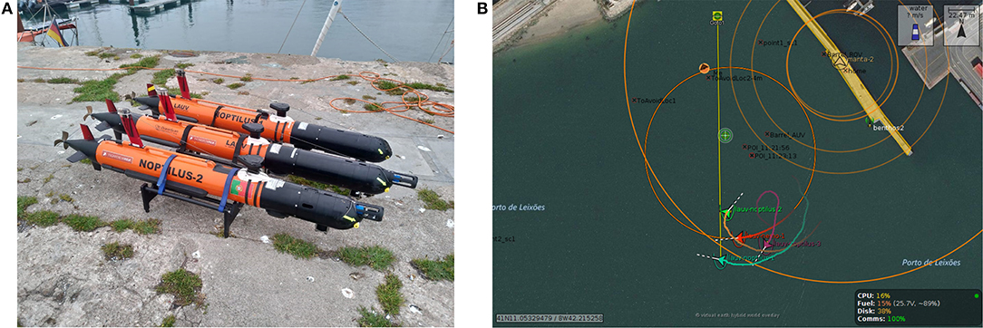
Figure 2. (A) Autonomous underwater vehicles used on the experiments. (B) The Neptus console.

The vehicles operate under the DUNE/Neptus environments, which are part of a software toolchain (Pinto et al., 2013) developed and maintained by LSTS. DUNE is the on-board software running on the vehicles, comprising all the software needed for communications, navigation, control, maneuvering, plan execution and supervision of multiple types of robotic vehicles. The control algorithms were implemented on C++, using the available DUNE libraries. Neptus is a software used for command, control and monitoring, comprising many typical functions needed for a typical mission, such as planning, execution and post-mission analysis (Figure 2B).

A target vehicle was simulated and continuously sends its position and orientation (computed from GPS/IMU measurements using an extended Kalman filter (Braga et al., 2012) to the three follower vehicles through static UDP connections with a maximum frequency of 1Hz. The control algorithm for the target vehicle is a vector field method (Nelson et al., 2007) that is responsible to steer the vehicle along a circumference with radius equal to 60m in the clockwise direction at 0.5m/s. The desired moving paths for the follower AUVs are planar circumference centered at the target vehicle with phase difference of 2π/3 between them:

$\begin{array}{ll}{p}_{d,i}^t({\gamma }_i)=R\left[\begin{array}{c}cos({\gamma }_i/R+{\varphi }_i)\\ sin({\gamma }_i/R+{\varphi }_i)\end{array}\right],& (28)\end{array}$

where R = 25m, ϕ₁ = 0 rad, ϕ₂ = 2π/3 rad and ϕ₃ = − 2π/3 rad. Each vehicle sends its path variable to the neighbor vehicles with a frequency of 1Hz to maintain coordination, according to the consensus law (24) and Assumption 2.4. The consensus gains are $k_{c,i}=0.1,\forall i\in {I}$.

For the construction of the MPF errors e_i, the value ϵ = [1 0]^T was used. The controller gain matrices and error correction gains were chosen as K_{p, i} = diag(0.2, 0.2) and $k_{e,i}=2,\forall i\in {I}$. The reference for the path variable velocity is v_d = 1m/s.

Remark 4.1. We point out the fact that this particular kind of vehicles cannot generate reliable negative forward velocities due to its propeller design. Given the fact that control laws (10), (17) can generate negative forward velocities if the virtual point is behind the line-of-sight of the vehicle, a substitute controller was designed to override the original controller in case this happens.

Therefore, while the forward velocity generated by (10) or (17) is negative (v_{f, i} < 0), the applied control signal will be

$\begin{array}{l}{u}_i=\left[\begin{array}{c}{v}_C\\ -sgn({\left[e_i\right]}_y-{ϵ}_2){\omega }_C\end{array}\right]\end{array}$

instead, until (10), (17) generate a positive v_{f, i} again. Constants v_C, ω_C ∈ ℝ are strictly positive. That means that the vehicle performs a “turning” maneuver with constant velocities until the virtual point is once again inside its line-of-sight. The direction of the turn is clockwise if the virtual point is to the right of the vehicle and counterclockwise if the virtual point is to the left of the vehicle. This strategy allows arbitrary initial configurations of the vehicles with respect to the initial position of the virtual point, and also allows the vehicles to recover from practical dead lock situations where their line-of-sight is kept facing away from the virtual point, which could happen, for example, in case of communication losses. In this case, v_C = 1.7m/s and ω_C = 1rad/s, approximately the upper saturation limits for the actuators.

4.2. Experimental Results

4.2.1. CMPF With Velocity Compensation

The first experiment shows the results of the CMPF controller with velocity compensation, ρ_i = 0 and no disturbance compensation (${\widehat{d}}_{v,i}=0$ and ${\widehat{d}}_{\omega ,i}=0$). Figure 3 shows the trajectories of the vehicles. The trajectory of the target is represented as the dashed black circle, in the clockwise direction. The small colored circles represent the beginning of the trajectory, while the colored asterisks represent its end. Noticeably, the three vehicles try to follow their respective paths (shown in dashed lines) around the rotating target, while maintaining their phase difference. Figure 4 shows the obtained results. The initial position of the vehicles was distant from the network router (located closer to the northeast part of Figure 3), which affected the wireless communications for a while. However, the initially large path variable errors rapidly decrease and remain bounded to less than 4 m (Figure 4B). Because of the communication losses and possibly the presence of ocean currents, the secondary controller described in Remark 3.5 had to recover some vehicles during the transient, resulting in some of the turning maneuvers we see in the beginning of the trajectories (Figure 3). After that transient, the norm of the MPF errors converge to a small region of less than 3 m while the control signal remains inside its linear region (Figures 4C,D). Note how the consensus law acts precisely when the path variable errors are high (Figure 4E), how the error correction terms acts when the MPF error norm is high (to prevent the evolution of the path variables), and how the rotation correction terms is fixed to a small value (≈ 0.18m/s) during the whole experiment. This is due to the fact that the target moves with constant angular velocity and the paths are circles to all three vehicles (see 23).

FIGURE 3

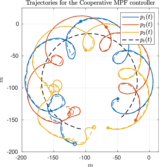
Figure 3. Vehicle trajectories for the CMPF controller with velocity compensation.

FIGURE 4

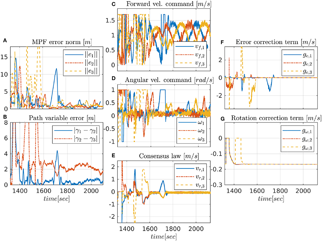
Figure 4. Experimental results for the CMPF controller with velocity compensation.

4.2.2. Robust CMPF With Sliding Mode Term

The second experiment shows the results of the robust CMPF controller with velocity compensation and Sliding Mode term, with MPF control law given by (10) with ρ_i = 0.2 for the three vehicles and ϵ_w = 0.5m. The consensus law for cooperation among the vehicles is given by (24), as before. Figure 5 shows the vehicle trajectories around the target, starting and ending in the southwest and southeast corners, respectively. Once more, due to communication losses and the presence of ocean currents in the southwest location, the secondary controller described in Remark 3.5 was activated for some of vehicles during the transient. However, the proposed controller was able to stabilize the error faster than the nominal controller. Besides, from Figure 6A, it is possible to notice the practical sliding mode phenomena around the origin e_i ≡ 0. That means that the controller is able to achieve better performance than the previous one, given that ϵ_w can be designed to be arbitrarily small. However, from (11), small values of ϵ_w can result in higher gains for w_i, which can potentially saturate the control inputs. In fact, sometimes the control saturation limits are reached after the transient, as shown in Figures 6C,D, and practical sliding mode is momentarily lost. The reason is the limited velocity range allowed by the actuators, combined with our particular value choice for ϵ_w, and moments of occasional increase in the target velocity. Even so, performance is slightly better than in the previous case, and the amount of control chattering is acceptable.

FIGURE 5

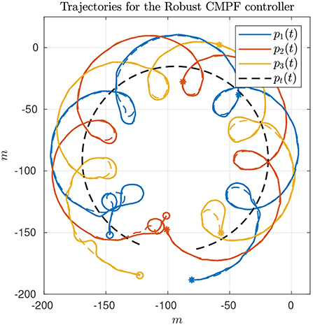
Figure 5. Vehicle trajectories for the robust CMPF controller.

FIGURE 6

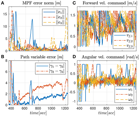
Figure 6. Results for the robust CMPF controller.

The consensus law, error correction signals and rotation correction signals are omitted, but are similar to those observed in Figure 4.

4.2.3. Robust CMPF With Sliding Mode Term and Disturbance Compensation

The third and last experiment shows the results of the robust CMPF controller with velocity compensation, Sliding Mode term and direct disturbance compensation using a linear observer. The control law is given by (17) with ρ_i = 0.2 and ϵ_w = 0.5m, as before. Again, the consensus law for cooperation among the vehicles is given by (24).

As seen from Figure 7, only the vehicles Noptilus 1 and 3 were used on this experiment, since the battery on Noptilus 2 was depleted. However, the results obtained by Noptilus 1 and 3 can still be compared to the previous results obtained for the same two vehicles. The chosen paths are the same circles defined in (28), but this time with ϕ₁ = 0 and ϕ₃ = πrad. This modification was used to guarantee that the two vehicles stay as far as possible from each another. Once again, in Figure 8A, notice the practical sliding mode phenomena around the origin e_i ≡ 0, except during the instants where the control inputs are saturated (Figures 8C,D). However, in this case, the control chattering is significantly smaller than the one observed in Figures 6C,D, under the same experimental conditions. We explain this fact by the presence of the disturbance estimator. Since part of the disturbance is compensated, the sliding mode term can spend less effort compensating the remaining total disturbance, a result compatible with the theoretical insight of Remark 3.2. The path variable errors remain bounded by 4m, as shown in Figure 8B. The estimated disturbances are shown in Figure 9. The linear velocity disturbances remained bounded by < 0.3ms after the transient, while the angular velocity disturbances showed higher variation, but remained bounded to < 0.5rads after the transient.

FIGURE 7

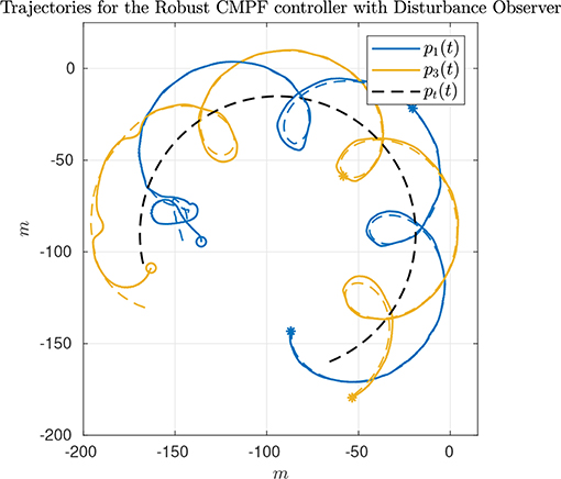
Figure 7. Vehicle trajectories for the robust CMPF controller with disturbance observer.

FIGURE 8

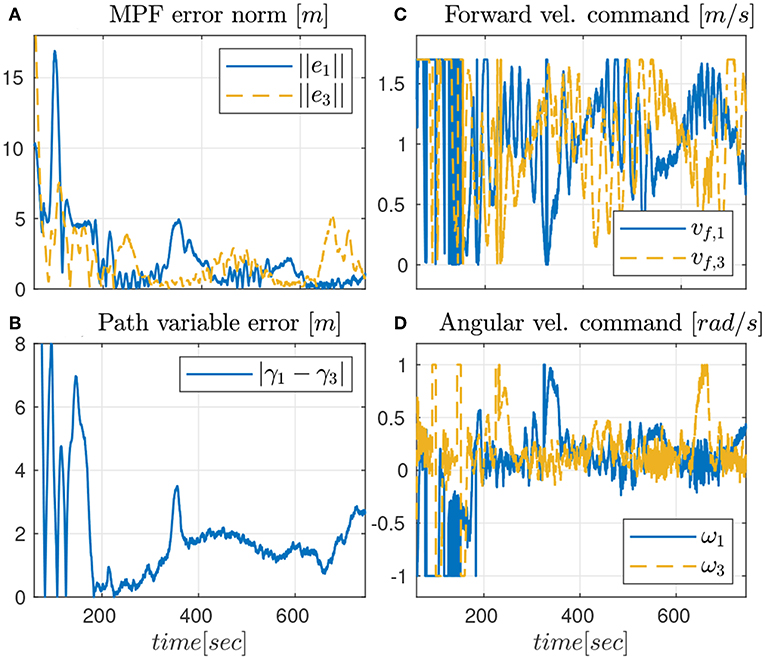
Figure 8. Results for the robust CMPF controller with disturbance observer.

FIGURE 9

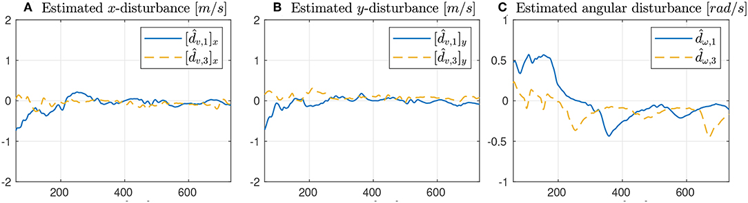
Figure 9. Results obtained with the disturbance estimator.

5. Conclusions

This work addressed the robust cooperative MPF problem for marine vehicles. We demonstrated that the origin of the MPF errors associated to the vehicles are stable with the two proposed robust CMPF control schemes in the presence of bounded disturbances acting on the vehicles. Furthermore, it was theoretically demonstrated that the cooperative control scheme is ISS with respect to the path variable estimation errors and to two other bounded, auxiliary input variables, named error correction term and rotation correction terms. The proposed robust controllers (10, 17) guarantee that the MPF error is globally uniformly bounded to a small neighborhood of the origin while maintaining acceptable control chattering. The narrow linear region of the actuators imposes limits on how small ϵ_w can be designed in practice. Lastly, we conclude that control law (17) actually improved the control chattering in practice, corroborating the theoretical insight of Remark 3.2.

Some of the future works are: (i) to investigate how to extend the proposed controllers to the case of unknown bounds for the disturbances (ii) to take the existence of actuator saturation limits in the control design and (iii) to incorporate obstacle avoidance techniques into the cooperative MPF approach to prevent vehicle collision during the cooperation tasks.

Data Availability Statement

The datasets generated for this study are available on request to the corresponding author.

Author Contributions

MR has written the manuscript, implemented the algorithms in C++ code, and performed the experiments using the LSTS vehicles. He also proposed the sliding mode based scheme for adding robustness to the moving path following controllers. RJ has proposed the cooperative control scheme using a consensus law, and contributed significantly to the stability proof of the cooperative controller. He also helped by suggesting important changes on the code and with the organization of the manuscript. AA contributed with the proposition of the disturbance compensation method for improving the performance of the first controller (Theorem 2), and also strongly contributed to the stability proofs and overall organization of the paper. JS made the experiments possible by setting up the mission at Porto de Leixões and has contributed by suggesting some changes on the code.

Funding

This work was supported in part by projects POCI-01-0145-FEDER-031823 - IMPROVE, and POCI-01-0145-FEDER-031411 - HARMONY, both funded by FEDER funds through COMPETE2020 - POCI and by national funds (PIDDAC), and also by project POCI-01-0247-FEDER-024508 - OceanTech, approved through the Incentive Scheme R&TD Co-promotion Projects and co-funded by the European Regional Development Fund, supported by Portugal2020 through Compete2020.

Conflict of Interest

The authors declare that the research was conducted in the absence of any commercial or financial relationships that could be construed as a potential conflict of interest.

Acknowledgments

The authors would like to acknowledge the support of the LSTS staff in conducting the experiments on Porto de Leixões. The code used in the experiments was written in C++ and can be accessed from the GITHUB® account on https://github.com/CaipirUltron/dune. The video to the experiments can be found at https://www.youtube.com/watch?v=qFNnGjBHqPk.

Footnotes

1. ^Khalil (2002) A nonlinear system $\stackrel{\bullet }{\delta }=f(t,\delta ,ϵ)$ is said to be Input-to-State Stable (ISS) if there exist a class ${K}{L}$ function β and a class ${K}$ function γ such that for any initial state δ(t₀) and any bounded input ϵ(t), the solution δ(t) exists for all t ≥ t₀ and satisfies

$\parallel \delta (t)\parallel \le \beta (\parallel \delta (t_0)\parallel ,t-t_0)+\gamma \left({\displaystyle \underset{t_0\le \tau \le t}{sup}}\parallel ϵ(\tau )\parallel \right)$

References

Aguiar, A. P. (2017). “Single and multiple motion control of autonomous robotic vehicles,” in 2017 11th International Workshop on Robot Motion and Control (RoMoCo) (Wasowo), 172–184. doi: 10.1109/RoMoCo.2017.8003910

CrossRef Full Text | Google Scholar

Aguiar, A. P., and Hespanha, J. P. (2007). Trajectory-tracking and path-following of underactuated autonomous vehicles with parametric modeling uncertainty. IEEE Trans. Automat. Control 52, 1362–1379. doi: 10.1109/TAC.2007.902731

CrossRef Full Text | Google Scholar

Aguiar, A. P., Hespanha, J. P., and Kokotovic, P. V. (2005). Path-following for nonminimum phase systems removes performance limitations. IEEE Trans. Automat. Cont. 50, 234–239. doi: 10.1109/TAC.2004.841924

CrossRef Full Text | Google Scholar

Aguiar, A. P., and Pascoal, A. M. (2002). “Dynamic positioning and way-point tracking of underactuated auvs in the presence of ocean currents,” in Proceedings of the 41st IEEE Conference on Decision and Control, 2002, Vol. 2 (Las Vegas, NV), 2105–2110.

Google Scholar

Aguiar, A. P., and Pascoal, A. M. (2007). “Coordinated path-following control for nonlinear systems with logic-based communication,” in 2007 46th IEEE Conference on Decision and Control (New Orleans, LA), 1473–1479. doi: 10.1109/CDC.2007.4434835

CrossRef Full Text | Google Scholar

Belleter, D., Paliotta, C., Maggiore, M., and Pettersen, K. (2016). “Path following for underactuated marine vessels. IFAC-PapersOnLine 49, 588–593. doi: 10.1016/j.ifacol.2016.10.229

CrossRef Full Text | Google Scholar

Braga, J., Healey, A. J., and Sousa, J. (2012). Navigation scheme for the lsts seacon vehicles: theory and application. IFAC Proc. Volumes 45, 69–75. doi: 10.3182/20120410-3-PT-4028.00013

CrossRef Full Text | Google Scholar

Cichella, V., Kaminer, I., Dobrokhodov, V., Xargay, E., Hovakimyan, N., and Pascoal, A. (2011). “Geometric 3D path-following control for a fixed-wing UAV on SO (3),” in AIAA Guidance, Navigation, and Control Conference (Portland, OR). doi: 10.2514/6.2011-6415

CrossRef Full Text | Google Scholar

Dagci, O. H., Ogras, U. Y., and Ozguner, U. (2003). “Path following controller design using sliding mode control theory,” in Proceedings of the 2003 American Control Conference, 2003, Vol. 1 (Denver, CO), 903–908.

Google Scholar

Encarnação, P., Pascoal, A., and Arcak, M. (2000). Path following for marine vehicles in the presence of unknown currents1. IFAC Proc. Volumes 33, 507–512. doi: 10.1016/S1474-6670(17)37980-6

CrossRef Full Text | Google Scholar

Gu, N., Peng, Z., Wang, D., Shi, Y., and Wang, T. (2019). Anti-disturbance coordinated path-following control of robotic autonomous surface vehicles: theory and experiment. IEEE/ASME Trans. Mechatr. 24 2386-2396. doi: 10.1109/TMECH.2019.2929216

CrossRef Full Text | Google Scholar

Jain, R. P., Aguiar, A. P., and de Sousa, J. B. (2018a). Cooperative path following of robotic vehicles using an event-based control and communication strategy. IEEE Robot. Automat. Lett. 3, 1941–1948. doi: 10.1109/LRA.2018.2808363

CrossRef Full Text | Google Scholar

Jain, R. P., Alessandretti, A., Aguiar, A. P., and De Sousa, J. B. (2018b). “Cooperative moving path following using event based control and communication,” in 2018 13th APCA International Conference on Automatic Control and Soft Computing (CONTROLO) (Ponta Delgada), 189–194.

Google Scholar

Jain, R. P. K., Aguiar, A. P., Alessandretti, A., and Borges de Sousa, J. (2018c). “Moving path following control of constrained underactuated vehicles: a nonlinear model predictive control approach,” in AIAA SciTech Forum (Kissimmee, FL: American Institute of Aeronautics and Astronautics).

Google Scholar

Kapitanyuk, Y. A., de Marina, H. G., Proskurnikov, A. V., and Cao, M. (2017). Guiding vector field algorithm for a moving path following problem. IFAC-PapersOnLine 50, 6983–6988. doi: 10.1016/j.ifacol.2017.08.1340

CrossRef Full Text | Google Scholar

Khalil, H. K. (2002). Nonlinear Systems, 3rd Edn. Upper Saddle River, NJ: Prentice-Hall.

Google Scholar

Micaelli, A., and Samson, C. (1993). Trajectory tracking for unicycle-type and two-steering-wheels mobile robots. Research Report RR-2097, INRIA. Available online at: https://hal.inria.fr/inria-00074575/file/RR-2097.pdf

Google Scholar

Nelson, D. R., Barber, D. B., McLain, T. W., and Beard, R. W. (2007). Vector field path following for miniature air vehicles. IEEE Trans. Robot. 23, 519–529. doi: 10.1109/TRO.2007.898976

CrossRef Full Text | Google Scholar

Olfati-Saber, R., Fax, J. A., and Murray, R. M. (2007). Consensus and cooperation in networked multi-agent systems. Proc. IEEE 95, 215–233. doi: 10.1109/JPROC.2006.887293

CrossRef Full Text | Google Scholar

Oliveira, T., Aguiar, A. P., and Encarnação, P. (2016). Moving path following for unmanned aerial vehicles with applications to single and multiple target tracking problems. IEEE Trans. Robot. 32, 1062–1078. doi: 10.1109/TRO.2016.2593044

CrossRef Full Text | Google Scholar

Oliveira, T., Aguiar, A. P., and Encarnação, P. (2017). “Three dimensional moving path following for fixed-wing unmanned aerial vehicles,” in 2017 IEEE International Conference on Robotics and Automation (ICRA) (Singapore), 2710–2716.

Google Scholar

Oliveira, T., and Encarnação, P. (2013). Ground target tracking control system for unmanned aerial vehicles. J. Intell. Robot. Syst. 69, 373–387. doi: 10.1007/s10846-012-9719-0

CrossRef Full Text | Google Scholar

Pinto, J., Dias, P. S., Martins, R., Fortuna, J., Marques, E., and Sousa, J. (2013). “The LSTS toolchain for networked vehicle systems,” in 2013 MTS/IEEE OCEANS-Bergen (Bergen: IEEE), 1–9.

Google Scholar

Reis, M. F., Jain, R. P., Aguiar, A. P., and de Sousa, J. B. (2019). Robust moving path following control for robotic vehicles: theory and experiments. IEEE Robot. Automat. Lett. 4, 3192–3199. doi: 10.1109/LRA.2019.2925733

CrossRef Full Text | Google Scholar

Samson, C. (1992). “Path following and time-varying feedback stabilization of a wheeled mobile robot,” in Second International Conference on Automation, Robotics and Computer Vision (Singapore), 3.

Google Scholar

Wang, R., Jing, H., Hu, C., Yan, F., and Chen, N. (2016). Robust H_∞ path following control for autonomous ground vehicles with delay and data dropout. IEEE Trans. Intell. Transport. Syst. 17, 2042–2050. doi: 10.1109/TITS.2015.2498157

CrossRef Full Text | Google Scholar

Xargay, E., Kaminer, I., Pascoal, A., Hovakimyan, N., Dobrokhodov, V., Cichella, V., et al. (2013). Time-critical cooperative path following of multiple uavs over time-varying networks. J. Guid. Cont. Dyn. 36, 499–516. doi: 10.2514/1.56538

CrossRef Full Text | Google Scholar

Zhang, L.-J., Jia, H.-M., and Jiang, D.-P. (2014). Sliding mode prediction control for 3d path following of an underactuated auv. IFAC Proc. Volumes 47, 8799–8804. doi: 10.3182/20140824-6-ZA-1003.00372

CrossRef Full Text | Google Scholar